1

Economics and the Geosciences

William D. Nordhaus AAAS Annual MeetingsYale University February 18, 2011

2

Outline of presentation

1. Economics and geography (GEcon)2. Economics and luminosity3. Integrated modeling of economics of climate

change (DICE/RICE)

3

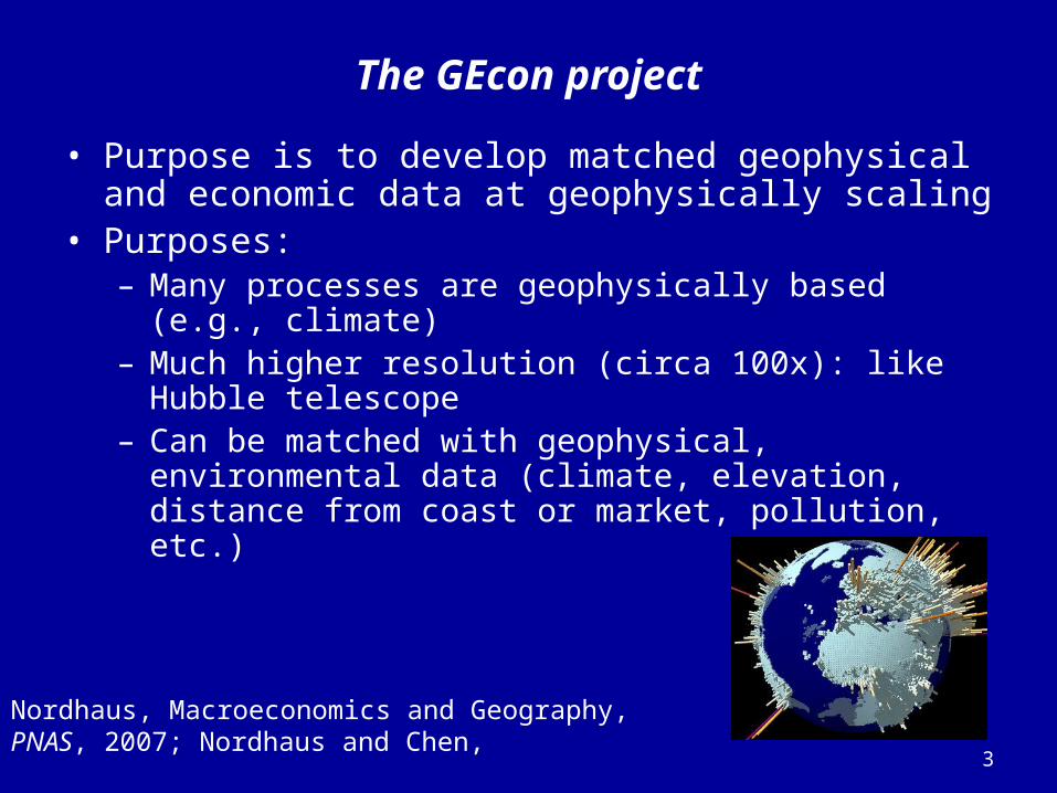
The GEcon project

• Purpose is to develop matched geophysical and economic data at geophysically scaling

• Purposes:– Many processes are geophysically based (e.g.,

climate)– Much higher resolution (circa 100x): like Hubble

telescope– Can be matched with geophysical, environmental

data (climate, elevation, distance from coast or market, pollution, etc.)

Nordhaus, Macroeconomics and Geography, PNAS, 2007; Nordhaus and Chen,

4

Derivation of Data Set

National or regional gross output,

population data

Regional (e.g., county)estimates of

output per capita

National and provincial GIS grid data (RIG, area, boundaries)

GPW grid cell estimates of

population, area, RIG

GEcon gross cellproduct (GCP)

data

Proportional allocation

from political to

geophysical boundaries

5

Countries and grid cells for Europe

6

Europe in 3D

Australia in 3D

7

Sydney

CanberraMelbourne

Perth

Darwin

Tasmania

8

Luminosity as a Proxy for Output

Xi ChenWilliam Nordhaus

Combining socioeconomic and luminosity data

Economic data on developing countries is very weak.

Question for this project: Can we use luminosity (nighttime lights) data as a proxy for standard accounting data for low-quality regions?

Allows use of regional GEcon data for rich regional data set.

9

Key elements in evaluating luminosity as a proxy

The key elements in determining the value of a proxy are:1. The quality of the luminosity data2. The errors of measurement of the standard GDP

data3. The statistical relationship between luminosity and

GDP

The background paper shows the optimal weighting as a signal-extraction statistical problem.

10

Chen and Nordhaus, The Value of Luminosity Data as a Proxy for Economic Statistics, NBER Working Paper, 2010

1111

Problems illustrated for southern New England

Bleeding

Saturation

Stable lights and output by 1° x 1° grid cell (n = 14,287)

12

-10

-8

-6

-4

-2

0

2

4

-15.0 -12.5 -10.0 -7.5 -5.0 -2.5 0.0

ln (output density)

ln (lu

min

osity

den

sity

)

Results on optimal weight on luminosity

13

0.0

0.2

0.4

0.6

0.8

1.0

A B C D E

Opti

mal

frac

tiona

l wei

ght o

n lu

min

osity

Country statistical quality grade (A = best; E = worst)

All regions

Low-density regions

Chen and Nordhaus, in process.

Main Results

1. For most countries, luminosity is essentially useless as a proxy for GDP and output measures.

2. Possible information value in statistical basket cases.

14

Economic Integrated Assessment (IA) Models

in Climate Change

15

16

Integrated Assessment (IA) Models in Climate Change

What are IA models?These are models that include the full range of cause and effect in climate change (“end to end” modeling).

Major goals of IA models:Project trends in consistent manner Assess costs and benefits of climate policies Estimate the carbon price and efficient emissions

reductions for different goals

Nordhaus, “Copenhagen Accord,” PNAS, 2010.

17

Fossil fuel usegenerates CO2

emissions

Carbon cycle: redistributes around

atmosphere, oceans, etc.

Climate system: change in radiative warming, precip,

ocean currents, sea level rise,…

Impacts on ecosystems,agriculture, diseases,

skiing, golfing, …

Measures to controlemissions (limits, taxes,

subsidies, …)

The emissions-climate-impacts-policy nexus:

The RICE-2010model

RICE-2010 model structure*

Economic module:- Standard economic production structure- GHG emissions are global externality - 12 regions, multiple periods

CO2/Climate module:

- Emissions = f(Q, carbon price, time)- Concentrations = g(emissions, diffusion)- Temperature change = h(GHG forcings, time lag)

- Economic damage = F(output, T, CO2, sea level rise)

* Nordhaus, “Economics of Copenhagen Accord,” PNAS (US), 2010.

19

1. Baseline.

2. Economic cost-benefit “optimum.”

3. Limit to 2 °C.

4. Copenhagen Accord, all countries.

5. Copenhagen Accord, rich only.

Policy Scenarios for Analysis using the RICE-2010 model

Temperature profiles: RICE -2010

20

0.0

1.0

2.0

3.0

4.0

5.0

6.0

2005 2025 2045 2065 2085 2105 2125 2145 2165 2185 2205

Glo

bal m

ean

tem

pera

ture

(deg

rees

C)

Optimal

Baseline

Lim T<2

Copen trade

Copen rich

Temperature

Source: Nordhaus, “Economics of Copenhagen Accord,” PNAS (US), 2010.

An interesting byproduct: CO2 shadow prices

Shadow prices (social costs) were discovered by developers of linear programming techniques (Kantorovich and Koopmans, Nobel 1974). Originally thought useful for central planning prices.

Today, useful because they reflect the marginal cost, or prices, of a constraint when efficiently imposed.

For example, IA models can calculate the price associated with the 2 °C temperature target as a byproduct of the economic models.

Can be used as guidelines for setting CO2 taxes or prices.

21

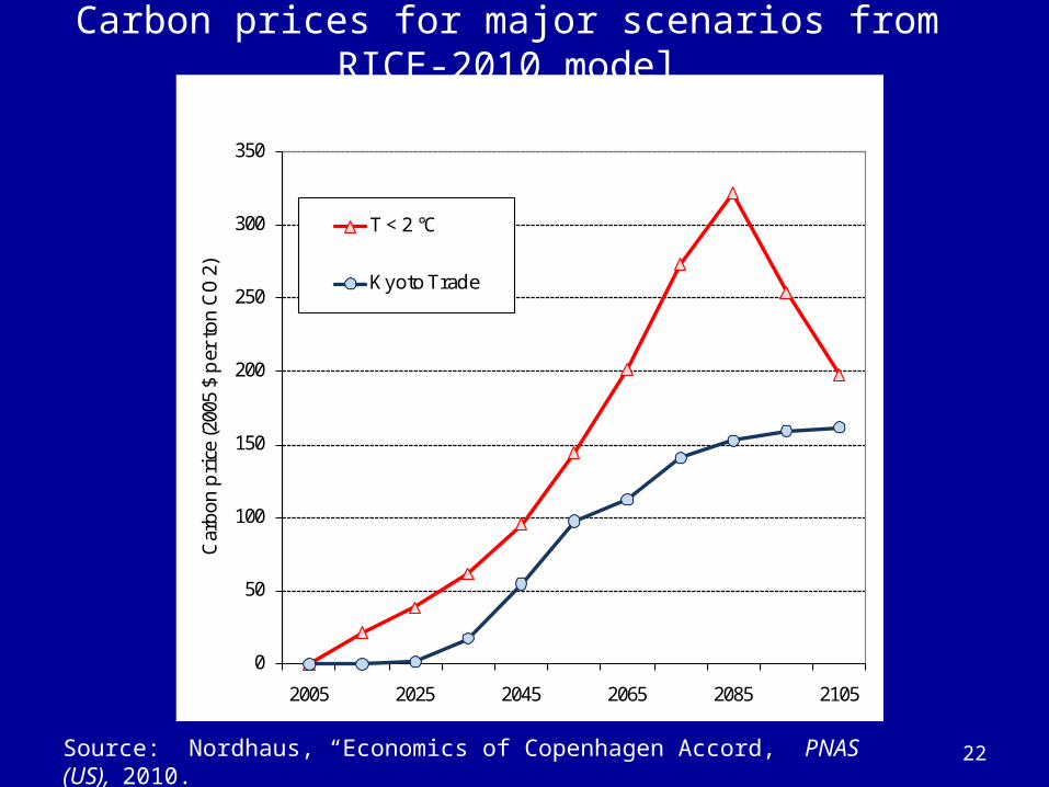
Carbon prices for major scenarios from RICE-2010 model

22Source: Nordhaus, “Economics of Copenhagen Accord,” PNAS (US), 2010.

0

50

100

150

200

250

300

350

2005 2025 2045 2065 2085 2105

Car

bon

pri

ce (2

005

$ per

ton

CO

2)T < 2 °C

Kyoto Trade

23

0

5

10

15

20

25

30

35

40

45

50

2005 2025

Car

bon

pri

ce (2

005

$ per

ton

CO

2)

T < 2 °C

Kyoto Trade

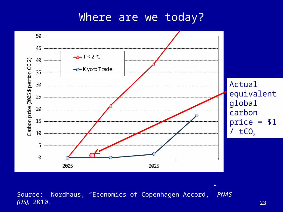
Where are we today?

23

Actual equivalent global carbon price = $1 / tCO2

Source: Nordhaus, “Economics of Copenhagen Accord,” PNAS (US), 2010.

24

A new scientific renaissance of social and

natural sciences?