11

Econ 240 CEcon 240 C

Lecture 6Lecture 6

22

Part I: Box-Jenkins MagicPart I: Box-Jenkins Magic

ARMA models of time series all built ARMA models of time series all built from one source, white noisefrom one source, white noise

33

Analysis and SynthesisAnalysis and Synthesis

White noise, WN(t) White noise, WN(t) Is a sequence of draws from a normal Is a sequence of draws from a normal

distribution, N(0, distribution, N(0, ), indexed by time), indexed by time

44

Analysis Analysis

Random walk, RW(t) Random walk, RW(t) Analysis formulation:Analysis formulation:RW(t) = RW(t-1) + WN(t)RW(t) = RW(t-1) + WN(t)RW(t) - RW(t-1) = WN(t)RW(t) - RW(t-1) = WN(t)RW(t) – Z*RW(t) = WN(t)RW(t) – Z*RW(t) = WN(t)[1 – Z]*RW(t) = WN(t)[1 – Z]*RW(t) = WN(t)*RW(t) = WN(t) shows how you turn a *RW(t) = WN(t) shows how you turn a

random walk into white noiserandom walk into white noise

55

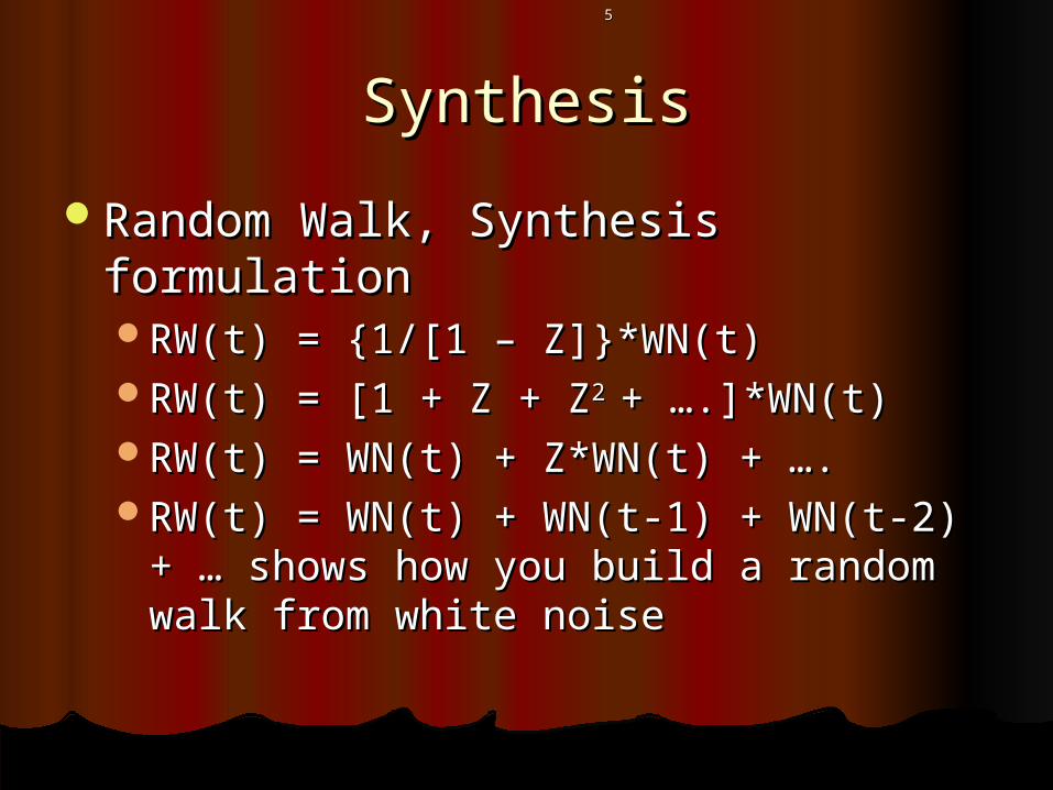
SynthesisSynthesis

Random Walk, Synthesis formulationRandom Walk, Synthesis formulationRW(t) = {1/[1 – Z]}*WN(t)RW(t) = {1/[1 – Z]}*WN(t)RW(t) = [1 + Z + ZRW(t) = [1 + Z + Z2 2 + ….]*WN(t)+ ….]*WN(t)RW(t) = WN(t) + Z*WN(t) + ….RW(t) = WN(t) + Z*WN(t) + ….RW(t) = WN(t) + WN(t-1) + WN(t-2) + … RW(t) = WN(t) + WN(t-1) + WN(t-2) + …

shows how you build a random walk shows how you build a random walk from white noisefrom white noise

66

AnalysisAnalysis

Autoregressive process of the first Autoregressive process of the first order, analysis formulationorder, analysis formulationARONE(t) = b*ARONE(t-1) + WN(t)ARONE(t) = b*ARONE(t-1) + WN(t)ARONE(t) - b*ARONE(t-1) = WN(t)ARONE(t) - b*ARONE(t-1) = WN(t)ARONE(t) - b*Z*ARONE(t) = WN(t)ARONE(t) - b*Z*ARONE(t) = WN(t)[1 – b*Z]*ARONE(t) = WN(t) is a quasi-[1 – b*Z]*ARONE(t) = WN(t) is a quasi-

difference and shows how you turn an difference and shows how you turn an autoregressive process of the first order autoregressive process of the first order into white noiseinto white noise

77

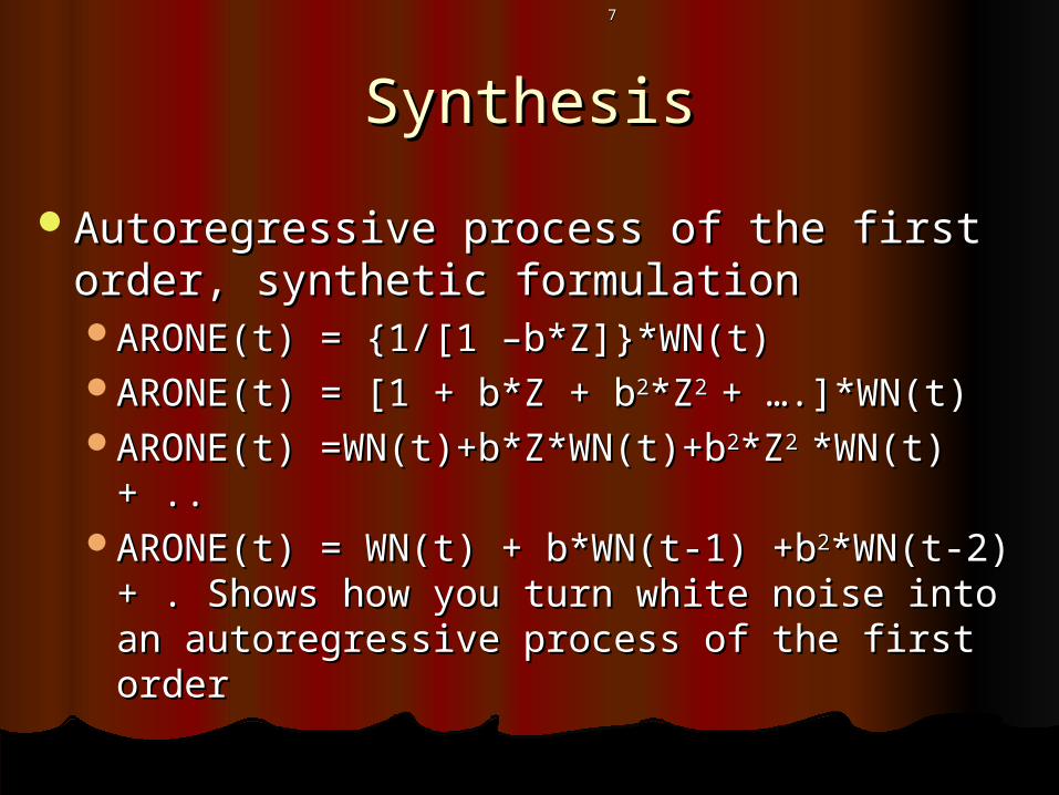
SynthesisSynthesis

Autoregressive process of the first order, Autoregressive process of the first order, synthetic formulationsynthetic formulationARONE(t) = {1/[1 –b*Z]}*WN(t)ARONE(t) = {1/[1 –b*Z]}*WN(t)ARONE(t) = [1 + b*Z + bARONE(t) = [1 + b*Z + b22*Z*Z2 2 + ….]*WN(t)+ ….]*WN(t)ARONE(t) =WN(t)+b*Z*WN(t)+bARONE(t) =WN(t)+b*Z*WN(t)+b22*Z*Z2 2 *WN(t) *WN(t)

+ ..+ ..ARONE(t) = WN(t) + b*WN(t-1) +bARONE(t) = WN(t) + b*WN(t-1) +b22*WN(t-2) *WN(t-2)

+ . Shows how you turn white noise into an + . Shows how you turn white noise into an autoregressive process of the first orderautoregressive process of the first order

88

Part II: Characterizing Time Part II: Characterizing Time Series BehaviorSeries Behavior

Mean function, m(t) = E [time_series(t)]Mean function, m(t) = E [time_series(t)]White noise: m(t) = E WN(t) = 0, all tWhite noise: m(t) = E WN(t) = 0, all tRandom walk: m(t) = E[WN(t)+WN(t-1) + ..] Random walk: m(t) = E[WN(t)+WN(t-1) + ..]

equals 0, all tequals 0, all tFirst order autoregressive process, First order autoregressive process,

m(t) = E[WN(t) + b*WN(t-1) + bm(t) = E[WN(t) + b*WN(t-1) + b22WN(t-2) + WN(t-2) + …] equals 0, all t…] equals 0, all t

Note that for all three types of time series we Note that for all three types of time series we calculate the mean function from the calculate the mean function from the synthetic expression for the time series. synthetic expression for the time series.

99

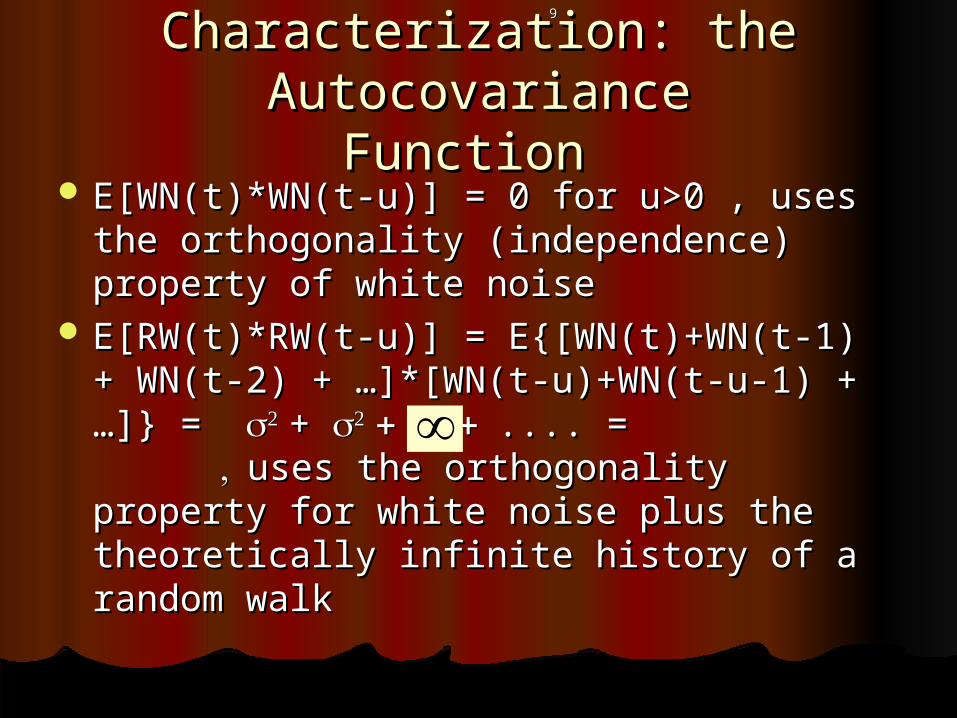
Characterization: the Characterization: the AutocovarianceAutocovariance

Function Function E[WN(t)*WN(t-u)] = 0 for u>0 , uses the E[WN(t)*WN(t-u)] = 0 for u>0 , uses the

orthogonality (independence) property orthogonality (independence) property of white noiseof white noise

E[RW(t)*RW(t-u)] = E{[WN(t)+WN(t-1) + E[RW(t)*RW(t-u)] = E{[WN(t)+WN(t-1) + WN(t-2) + …]*[WN(t-u)+WN(t-u-1) +…]} WN(t-2) + …]*[WN(t-u)+WN(t-u-1) +…]} = = + + .... = .... = uses the uses the orthogonality property for white noise orthogonality property for white noise plus the theoretically infinite history of a plus the theoretically infinite history of a random walkrandom walk

1010

The Autocovariance FunctionThe Autocovariance Function

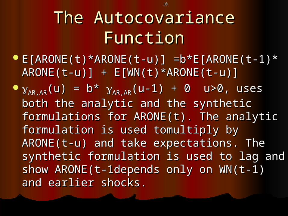
E[ARONE(t)*ARONE(t-u)] =b*E[ARONE(t-E[ARONE(t)*ARONE(t-u)] =b*E[ARONE(t-1)* ARONE(t-u)] + E[WN(t)*ARONE(t-u)]1)* ARONE(t-u)] + E[WN(t)*ARONE(t-u)]

AR,ARAR,AR(u) = b* (u) = b* AR,ARAR,AR(u-1) + 0 u>0, uses both (u-1) + 0 u>0, uses both the analytic and the synthetic formulations the analytic and the synthetic formulations for ARONE(t). The analytic formulation is for ARONE(t). The analytic formulation is used tomultiply by ARONE(t-u) and take used tomultiply by ARONE(t-u) and take expectations. The synthetic formulation is expectations. The synthetic formulation is used to lag and show ARONE(t-1depends used to lag and show ARONE(t-1depends only on WN(t-1) and earlier shocks.only on WN(t-1) and earlier shocks.

1111

The Autocorrelation FunctionThe Autocorrelation Function

x,xx,x(u) = (u) = AR,ARAR,AR(u)/ (u)/ AR,ARAR,AR(0) (0)

White Noise: White Noise: WN,WNWN,WN(u) = 0(u) = 0uu

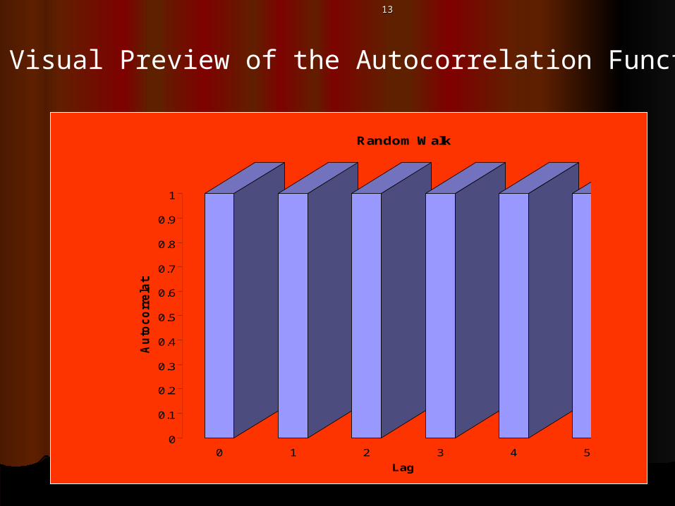
Random Walk: Random Walk: RW,RWRW,RW(u) = 1, all u(u) = 1, all u

Autoregressive of the first order: Autoregressive of the first order: x,xx,x(u) = (u) = bbuu

1212

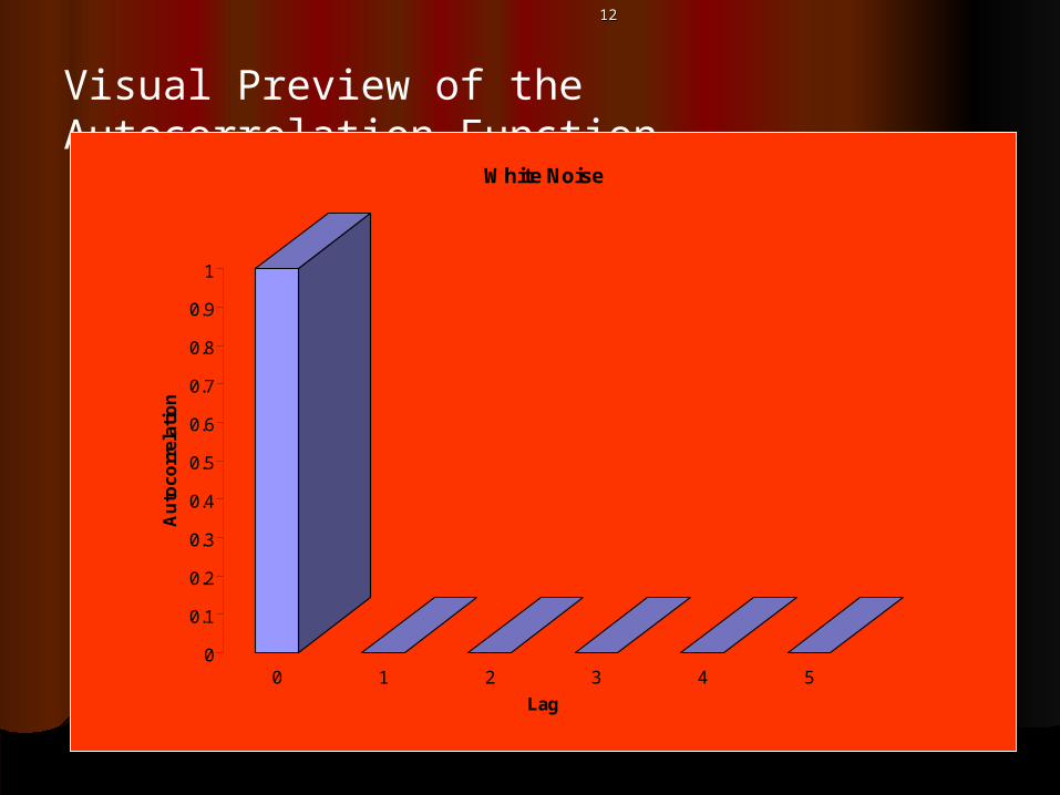
Visual Preview of the Autocorrelation Function

0

0.1

0.2

0.3

0.4

0.5

0.6

0.7

0.8

0.9

1

Au

toco

rrel

atio

n

0 1 2 3 4 5

Lag

White Noise

1313

Visual Preview of the Autocorrelation Function

0

0.1

0.2

0.3

0.4

0.5

0.6

0.7

0.8

0.9

1

Au

toc

orr

ela

tio

n

0 1 2 3 4 5

Lag

Random Walk

1414

Visual Preview of the Autocorrelation Function

0

0.1

0.2

0.3

0.4

0.5

0.6

0.7

0.8

0.9

1

Au

toco

rrel

atio

n

0 1 2 3 4 5

Lag

Autoregressive, 1st Order

1515

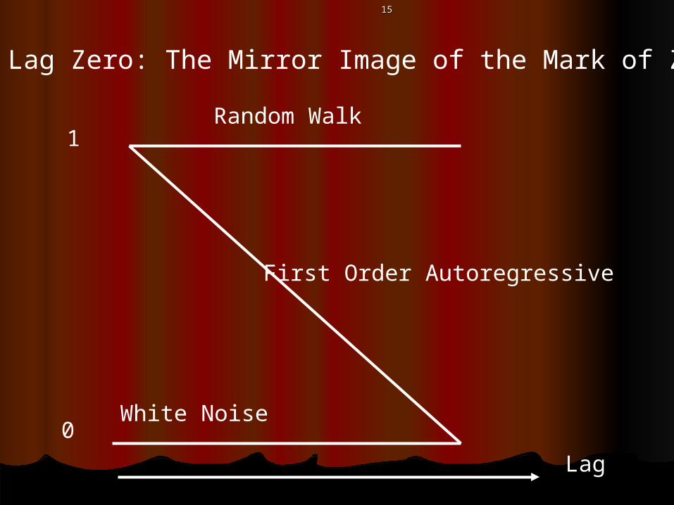
Drop Lag Zero: The Mirror Image of the Mark of Zorro

White Noise

First Order Autoregressive

Random Walk

Lag

1

0

1616

Part III.Analysis in the Lab: Part III.Analysis in the Lab: ProcessProcess

IdentificationIdentificationEstimationEstimationVerificationVerificationForecastingForecasting

1717

Analysis in the Lab: ProcessAnalysis in the Lab: Process

IdentificationIdentificationIs the time series stationary?Is the time series stationary?

TraceTraceHistogramHistogramAutocorrelation FunctionAutocorrelation Function

If it is, proceedIf it is, proceedIf it is not, difference (prewhitening)If it is not, difference (prewhitening)

1818

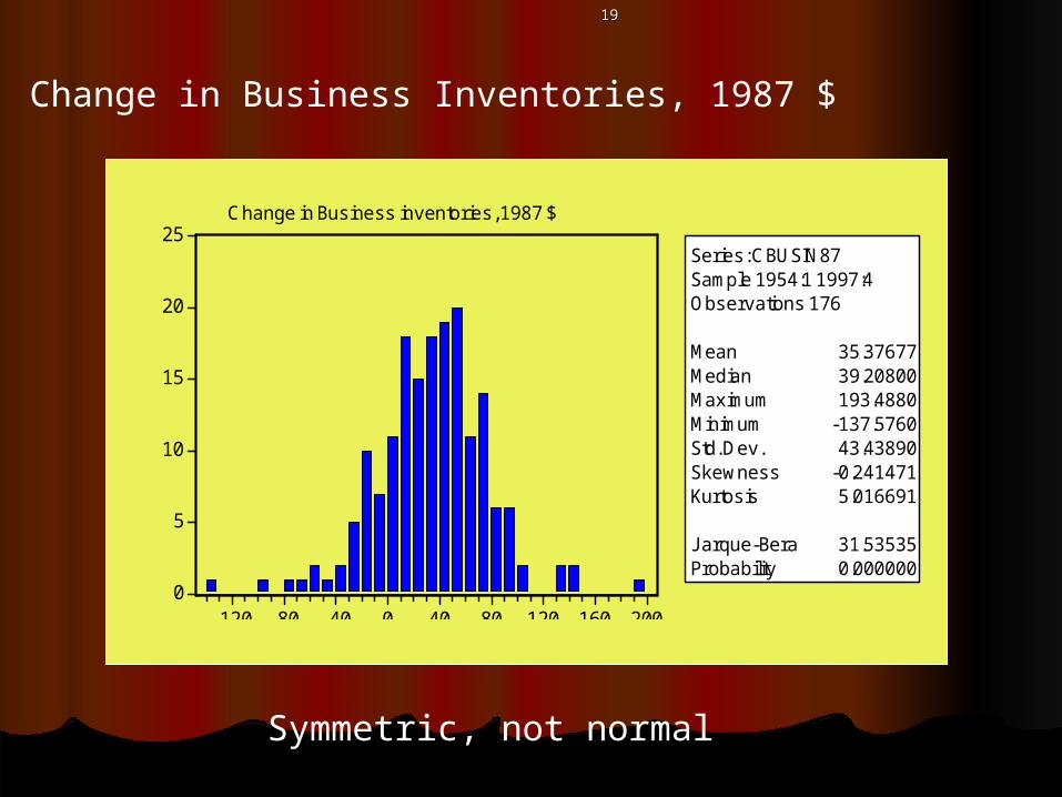
Change in Business Inventories, 1987 $

-200

-100

0

100

200

55 60 65 70 75 80 85 90 95

Change in Business Inventories, 1987 $

No trend, no seasonal

1919

Change in Business Inventories, 1987 $

0

5

10

15

20

25

-120 -80 -40 0 40 80 120 160 200

Series: CBUSIN87Sample 1954:1 1997:4Observations 176

Mean 35.37677Median 39.20800Maximum 193.4880Minimum -137.5760Std. Dev. 43.43890Skewness -0.241471Kurtosis 5.016691

Jarque-Bera 31.53535Probability 0.000000

Change in Business inventories, 1987 $

Symmetric, not normal

2020

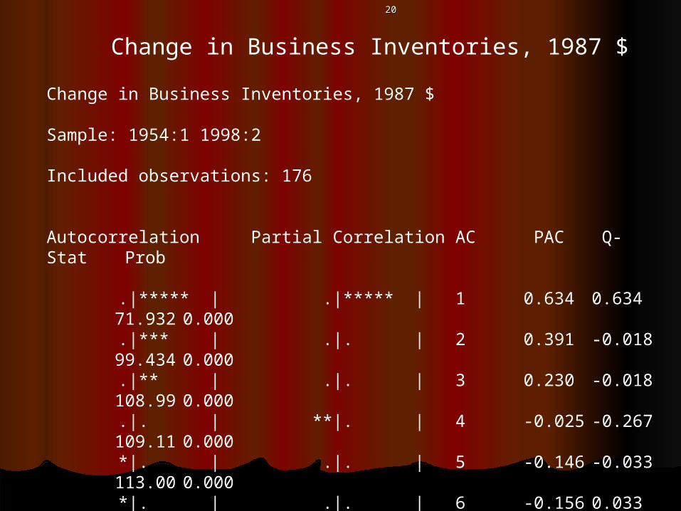
Change in Business Inventories, 1987 $

Change in Business Inventories, 1987 $

Sample: 1954:1 1998:2

Included observations: 176

Autocorrelation Partial CorrelationAC PAC Q-Stat Prob

.|***** | .|***** | 1 0.634 0.634 71.932 0.000

.|*** | .|. | 2 0.391 -0.018 99.434 0.000

.|** | .|. | 3 0.230 -0.018 108.99 0.000

.|. | **|. | 4 -0.025 -0.267 109.11 0.000

*|. | .|. | 5 -0.146 -0.033 113.00 0.000

*|. | .|. | 6 -0.156 0.033 117.46 0.000

*|. | .|. | 7 -0.153 0.011 121.83 0.000

*|. | .|. | 8 -0.128 -0.034 124.87 0.000

*|. | .|. | 9 -0.074 -0.008 125.90 0.000

.|. | .|. | 10 -0.001 0.057 125.90 0.000

.|. | .|. | 11 0.048 0.029 126.34 0.000

.|. | .|. | 12 0.055 -0.032 126.91 0.000

.|* | .|. | 13 0.069 0.010 127.84 0.000

2121

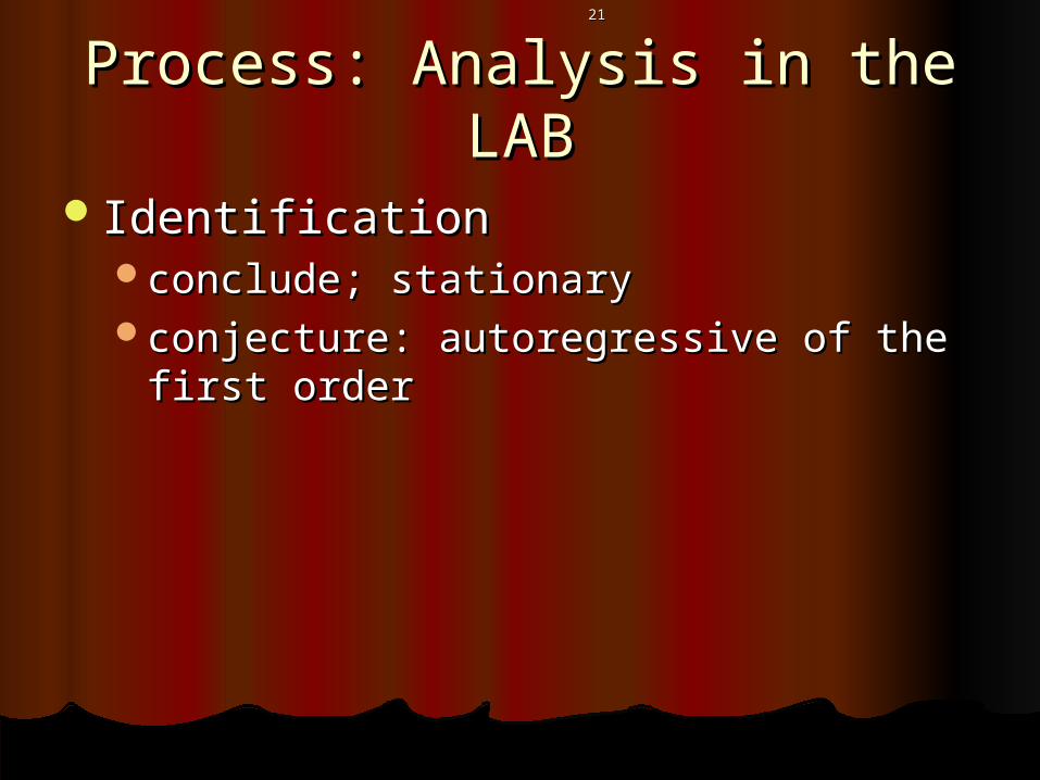
Process: Analysis in the LABProcess: Analysis in the LAB

IdentificationIdentificationconclude; stationaryconclude; stationaryconjecture: autoregressive of the first conjecture: autoregressive of the first

orderorder

2222

Process: Analysis in the LABProcess: Analysis in the LAB

EstimationEstimationEVIEWS model:EVIEWS model:

time series(t) = constant + residual(t)time series(t) = constant + residual(t)residual(t) =b*residual(t-1) + WN(t)?residual(t) =b*residual(t-1) + WN(t)?

Combine the two:Combine the two:[time series(t) - c] =b*[time series(t-1) - c] [time series(t) - c] =b*[time series(t-1) - c]

+WN(t)?+WN(t)?EVIEWS Specification:EVIEWS Specification:

cbusin87 c ar(1)cbusin87 c ar(1)

2323

Dependent Variable: CBUSIN87Method: Least Squares

Sample(adjusted): 1954:2 1997:4Included observations: 175 after adjusting endpoints

Convergence achieved after 3 iterations

Variable Coefficient Std. Error t-Statistic Prob.

C 36.58319 6.977023 5.243381 0.0000AR(1) 0.636816 0.058435 10.89788 0.0000

R-squared 0.407055 Mean dependent var 35.67438

Adjusted R-squared 0.403627 S.D. dependent var 43.38323

S.E. of regression 33.50278 Akaike info criterion 9.872497

Sum squared resid 194181.5 Schwarz criterion 9.908666

Log likelihood -861.8435 F-statistic 118.7638

Durbin-Watson stat 1.978452 Prob(F-statistic) 0.000000

Inverted AR Roots .64

2424

EstimationEstimation

Goodness of FitGoodness of FitStructure in the residuals? Are they Structure in the residuals? Are they

orthogonal?orthogonal?Are the residuals normally Are the residuals normally

distributed?distributed?

2525

-200

-100

0

100

200

-200

-100

0

100

200

55 60 65 70 75 80 85 90 95

Residual Actual Fitted

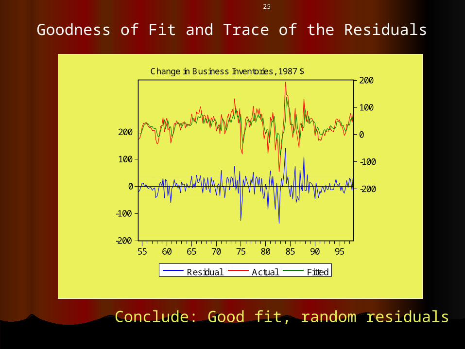
Change in Business Inventories, 1987 $

Goodness of Fit and Trace of the Residuals

Conclude: Good fit, random residuals

2626

ResidualsSample: 1954:2 1997:4Included observations: 175Q-statistic probabilities adjusted for 1 ARMA term(s)

Autocorrelation Partial CorrelationAC PAC Q-Stat Prob

.|. | .|. | 1 0.007 0.007 0.0095 .|. | .|. | 2 -0.007 -0.007 0.0187 0.891 .|* | .|* | 3 0.156 0.156 4.4132 0.110 *|. | *|. | 4 -0.145 -0.151 8.2199 0.042 *|. | *|. | 5 -0.150 -0.148 12.307 0.015 .|. | *|. | 6 -0.046 -0.071 12.688 0.026 *|. | .|. | 7 -0.058 -0.012 13.314 0.038 *|. | .|. | 8 -0.063 -0.040 14.055 0.050 .|. | *|. | 9 -0.042 -0.071 14.378 0.072 .|. | .|. | 10 0.023 -0.005 14.477 0.106 .|. | .|. | 11 0.054 0.046 15.020 0.131 .|. | .|. | 12 0.001 -0.011 15.021 0.182 .|. | .|. | 13 0.064 0.027 15.805 0.200

Correlogram of the Residuals

Conclude: (orthogonal)

2727

0

5

10

15

20

25

30

-120 -80 -40 0 40 80 120

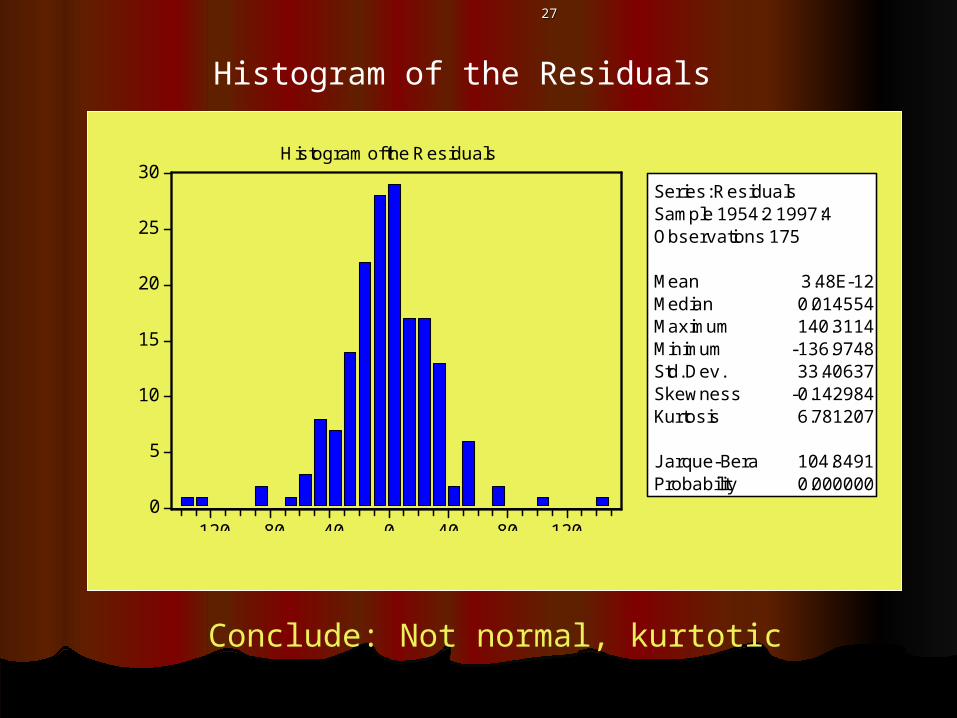
Series: ResidualsSample 1954:2 1997:4Observations 175

Mean 3.48E-12Median 0.014554Maximum 140.3114Minimum -136.9748Std. Dev. 33.40637Skewness -0.142984Kurtosis 6.781207

Jarque-Bera 104.8491Probability 0.000000

Histogram of the Residuals

Histogram of the Residuals

Conclude: Not normal, kurtotic

2828

Process: Analysis in the LABProcess: Analysis in the LAB

IdentificationIdentificationEstimationEstimationVerificationVerification

Is there any structure left in the Is there any structure left in the residuals? If not, we are back to our residuals? If not, we are back to our building block, orthogonal residuals, and building block, orthogonal residuals, and we accept the model.we accept the model.

2929

Process: Analysis in the LABProcess: Analysis in the LAB

IdentificationIdentificationEstimationEstimationVerificationVerification

Is there any structure left in the Is there any structure left in the residuals? If not, we are back to our residuals? If not, we are back to our building block, orthogonal residuals, and building block, orthogonal residuals, and we accept the model.we accept the model.

ForecastingForecastingone period ahead forecastsone period ahead forecasts

3030

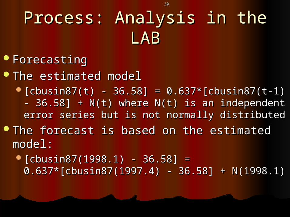
Process: Analysis in the LABProcess: Analysis in the LAB

ForecastingForecastingThe estimated modelThe estimated model

[cbusin87(t) - 36.58] = 0.637*[cbusin87(t-1) - [cbusin87(t) - 36.58] = 0.637*[cbusin87(t-1) - 36.58] + N(t) where N(t) is an independent 36.58] + N(t) where N(t) is an independent error series but is not normally distributederror series but is not normally distributed

The forecast is based on the estimated The forecast is based on the estimated model:model:[cbusin87(1998.1) - 36.58] = [cbusin87(1998.1) - 36.58] =

0.637*[cbusin87(1997.4) - 36.58] + N(1998.1)0.637*[cbusin87(1997.4) - 36.58] + N(1998.1)

3131

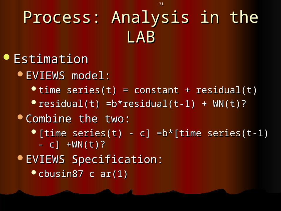
Process: Analysis in the LABProcess: Analysis in the LAB

EstimationEstimationEVIEWS model:EVIEWS model:

time series(t) = constant + residual(t)time series(t) = constant + residual(t)residual(t) =b*residual(t-1) + WN(t)?residual(t) =b*residual(t-1) + WN(t)?

Combine the two:Combine the two:[time series(t) - c] =b*[time series(t-1) - c] [time series(t) - c] =b*[time series(t-1) - c]

+WN(t)?+WN(t)?EVIEWS Specification:EVIEWS Specification:

cbusin87 c ar(1)cbusin87 c ar(1)

3232

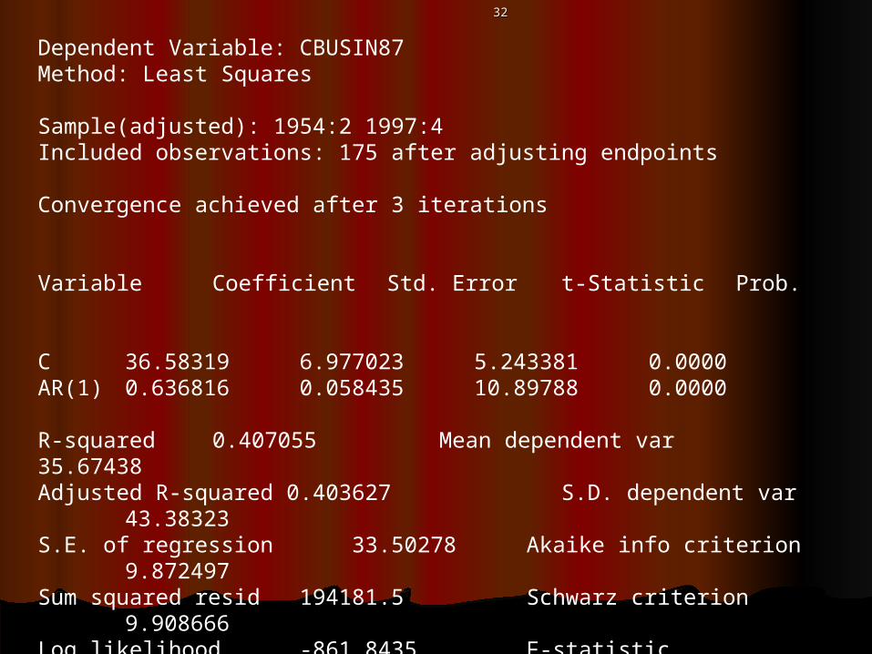
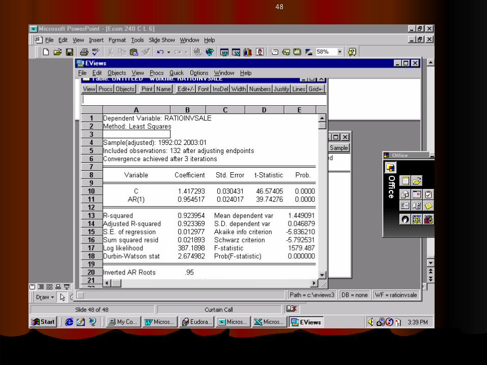
Dependent Variable: CBUSIN87Method: Least Squares

Sample(adjusted): 1954:2 1997:4Included observations: 175 after adjusting endpoints

Convergence achieved after 3 iterations

Variable Coefficient Std. Error t-Statistic Prob.

C 36.58319 6.977023 5.243381 0.0000AR(1) 0.636816 0.058435 10.89788 0.0000

R-squared 0.407055 Mean dependent var 35.67438

Adjusted R-squared 0.403627 S.D. dependent var 43.38323

S.E. of regression 33.50278 Akaike info criterion 9.872497

Sum squared resid 194181.5 Schwarz criterion 9.908666

Log likelihood -861.8435 F-statistic 118.7638

Durbin-Watson stat 1.978452 Prob(F-statistic) 0.000000

Inverted AR Roots .64

3333

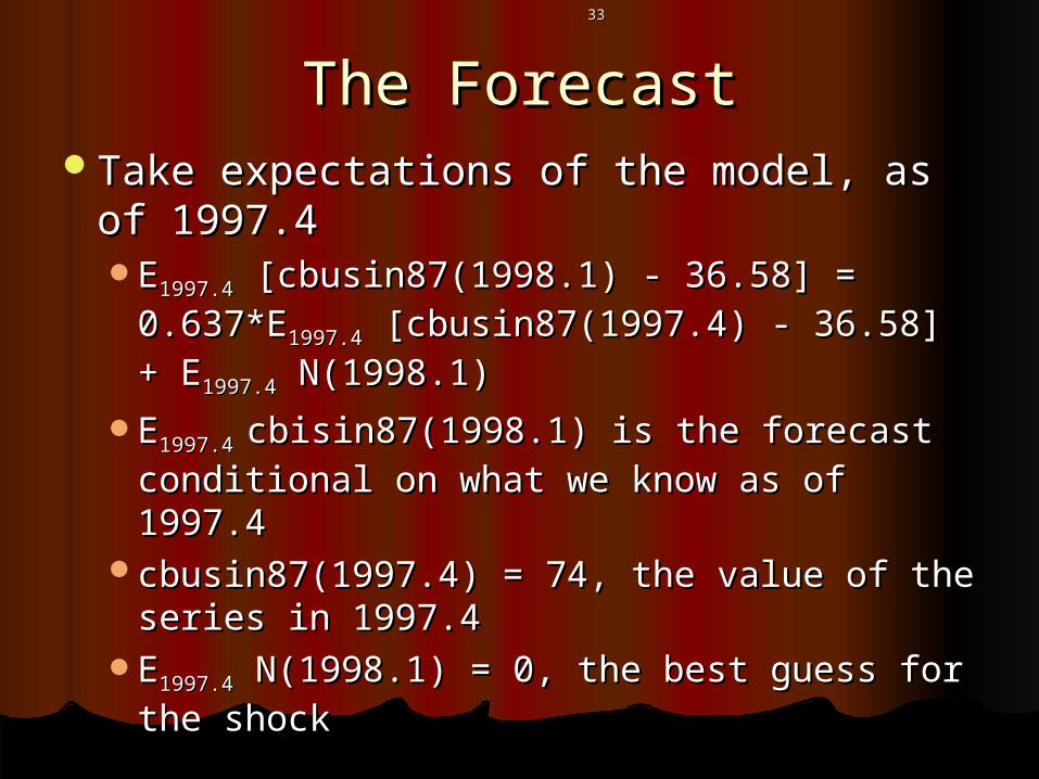
The ForecastThe ForecastTake expectations of the model, as of Take expectations of the model, as of

1997.41997.4EE1997.41997.4 [cbusin87(1998.1) - 36.58] = [cbusin87(1998.1) - 36.58] =

0.637*E0.637*E1997.41997.4 [cbusin87(1997.4) - 36.58] + [cbusin87(1997.4) - 36.58] + EE1997.41997.4 N(1998.1) N(1998.1)

EE1997.4 1997.4 cbisin87(1998.1) is the forecast cbisin87(1998.1) is the forecast conditional on what we know as of 1997.4conditional on what we know as of 1997.4

cbusin87(1997.4) = 74, the value of the cbusin87(1997.4) = 74, the value of the series in 1997.4series in 1997.4

EE1997.41997.4 N(1998.1) = 0, the best guess for N(1998.1) = 0, the best guess for the shockthe shock

3434

The ForecastThe Forecast

Calculate the forecast by handCalculate the forecast by handfor a one period ahead forecast, the for a one period ahead forecast, the

standard error of the regression can standard error of the regression can be used for the standard error of the be used for the standard error of the forecastforecast

calculate the upper band: forecast+ calculate the upper band: forecast+ 2*SER2*SER

calculate the lower band: forecast - calculate the lower band: forecast - 2*SER2*SER

3535

The ForecastThe Forecast

Use EVIEWS as a checkUse EVIEWS as a check

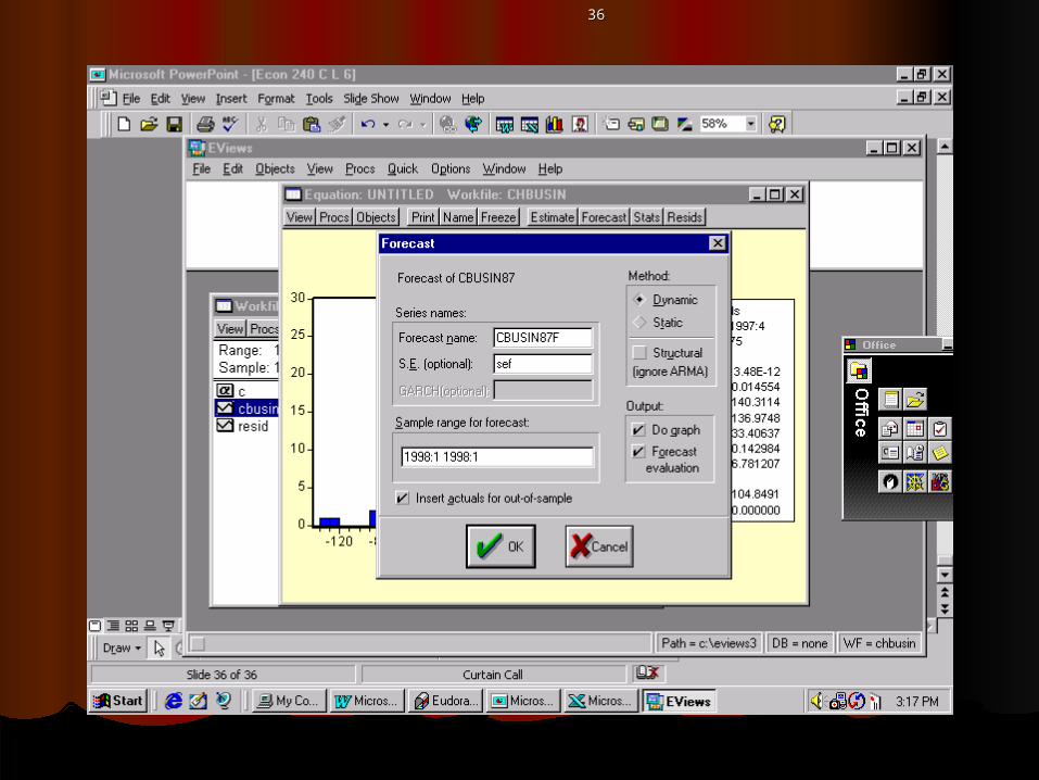
3636

3737

-20

0

20

40

60

80

100

120

140

1998:1

CBUSIN87F ± 2 S.E.

95 % Confidence Intervals and the Forecast, Visual

3838

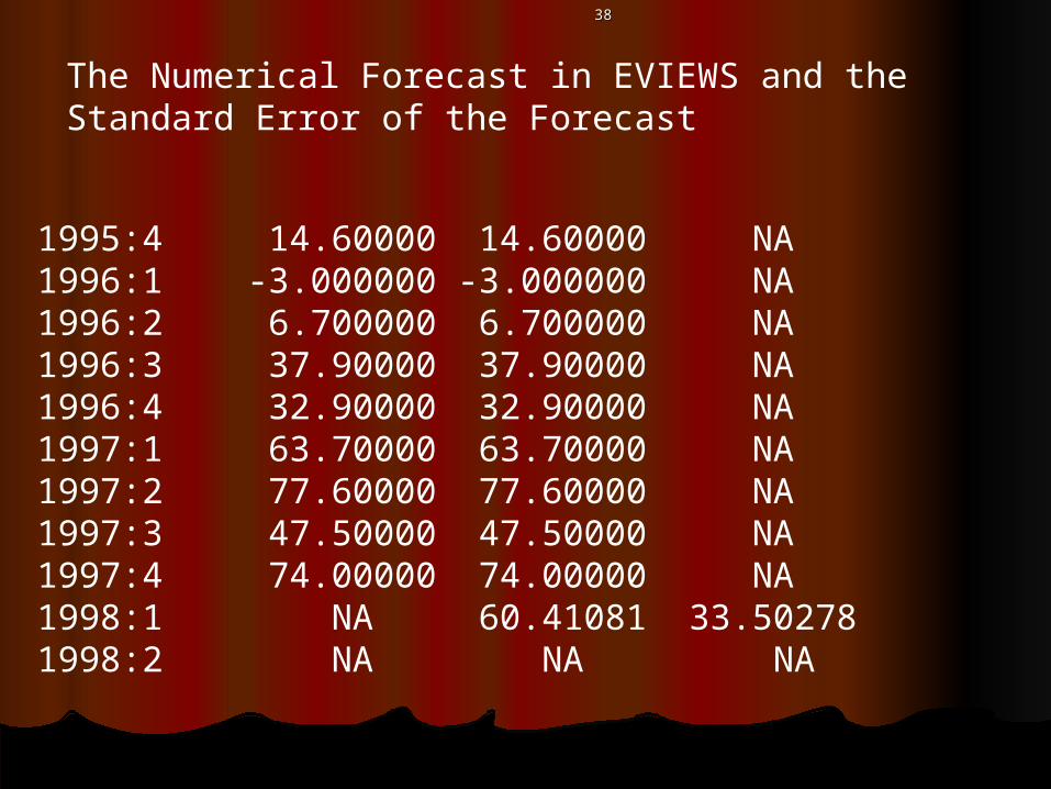
1995:4 14.60000 14.60000 NA 1996:1 -3.000000 -3.000000 NA 1996:2 6.700000 6.700000 NA 1996:3 37.90000 37.90000 NA 1996:4 32.90000 32.90000 NA 1997:1 63.70000 63.70000 NA 1997:2 77.60000 77.60000 NA 1997:3 47.50000 47.50000 NA 1997:4 74.00000 74.00000 NA 1998:1 NA 60.41081 33.502781998:2 NA NA NA

The Numerical Forecast in EVIEWS and the Standard Error of the Forecast

3939

Part IV. Process: Fill in the Part IV. Process: Fill in the BlanksBlanks

The ratio of inventories to sales, total The ratio of inventories to sales, total businessbusiness

4040

What is the first step?What is the first step?

4141

1992:01 1.5600001992:02 1.5600001992:03 1.5400001992:04 1.5300001992:05 1.5300001992:06 1.5200001992:07 1.5100001992:08 1.5400001992:09 1.5200001992:10 1.5200001992:11 1.5200001992:12 1.5300001993:01 1.5000001993:02 1.510000

2003:01 1.36

spreadsheet

4242

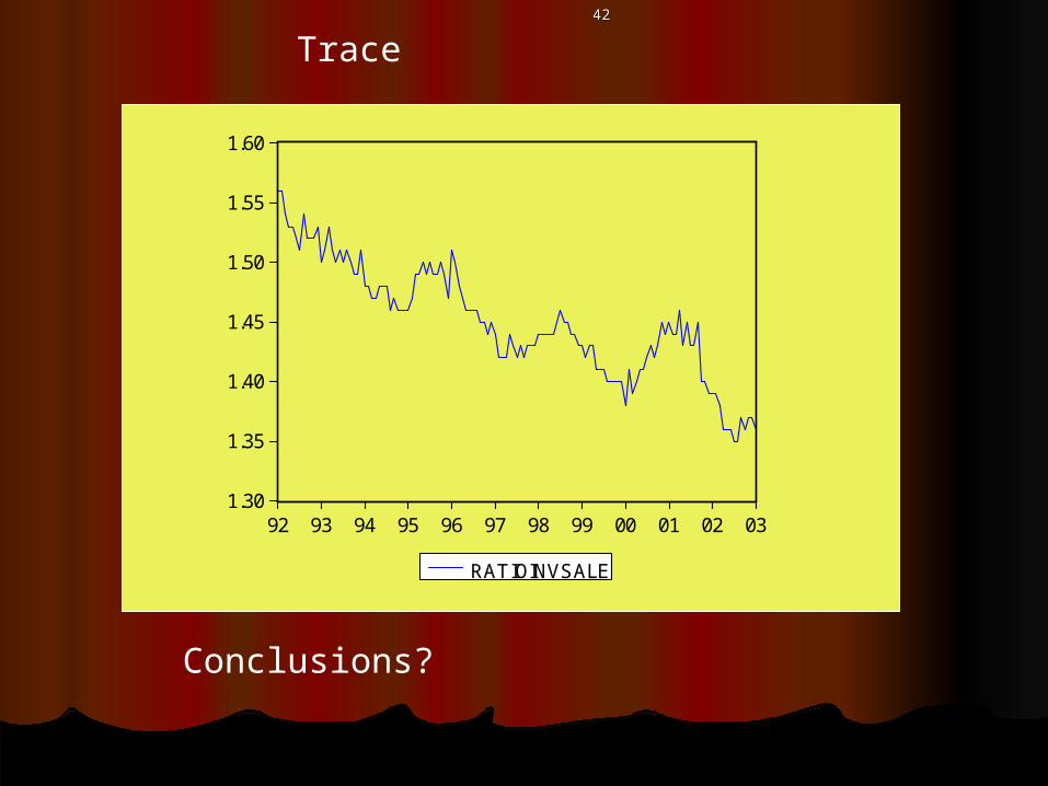
1.30

1.35

1.40

1.45

1.50

1.55

1.60

92 93 94 95 96 97 98 99 00 01 02 03

RATIOINVSALE

Conclusions?

Trace

4343

0

4

8

12

16

1.35 1.40 1.45 1.50 1.55

Series: RATIOINVSALESample 1992:01 2003:01Observations 133

Mean 1.449925Median 1.450000Maximum 1.560000Minimum 1.350000Std. Dev. 0.047681Skewness 0.027828Kurtosis 2.475353

Jarque-Bera 1.542537Probability 0.462426

Histogram

Conclusions?

4444

Correlogram Conclusions?

4545

What is the Next Step?What is the Next Step?

4646

Conjecture: ModelConjecture: Model

4747

What do we do now?What do we do now?

4848

4949

What do we do next?What do we do next?

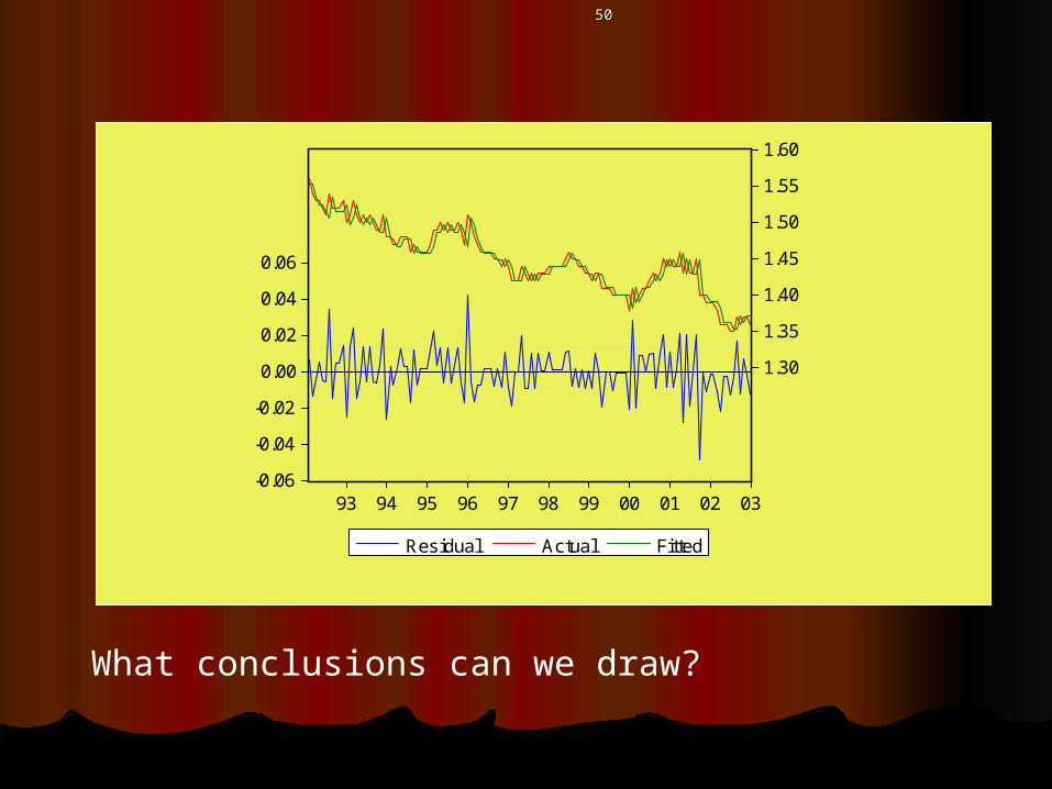
5050

-0.06

-0.04

-0.02

0.00

0.02

0.04

0.06

1.30

1.35

1.40

1.45

1.50

1.55

1.60

93 94 95 96 97 98 99 00 01 02 03

Residual Actual Fitted

What conclusions can we draw?

5151

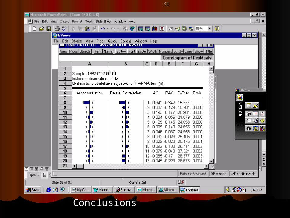
Conclusions

5252

0

5

10

15

20

25

-0.050 -0.025 0.000 0.025

Series: ResidualsSample 1992:02 2003:01Observations 132

Mean -2.74E-13Median 0.000351Maximum 0.042397Minimum -0.048512Std. Dev. 0.012928Skewness 0.009594Kurtosis 4.435641

Jarque-Bera 11.33788Probability 0.003452

5353

If we accepted this model, If we accepted this model, what would the formula be?what would the formula be?

Ratioinvsale(t) Ratioinvsale(t)

5454Make a one period ahead Make a one period ahead forecast; what is the standard forecast; what is the standard

error of the forecast?error of the forecast?