1

Ecological nonlinearities inform the design of functional flows for imperiled 1

fish in a highly modified river 2

Running head: Salmon survival informs functional flows 3

Cyril J. Michel1*, Jeremy J. Notch1, Flora Cordoleani1, Eric M. Danner2

* Corresponding author

cyril.michel@noaa.gov

Voice: 831-420-3986

1 University of California, Santa Cruz

Institute of Marine Sciences

Affiliated with:

Southwest Fisheries Science Center - Fisheries Ecology Division

National Marine Fisheries Service

National Oceanic and Atmospheric Administration

110 McAllister Way, Santa Cruz, CA 95060

2 Southwest Fisheries Science Center - Fisheries Ecology Division

National Marine Fisheries Service

National Oceanic and Atmospheric Administration

110 McAllister Way, Santa Cruz, CA 95060

4

2

ABSTRACT 5

Water is a fundamental resource in freshwater ecosystems, and streamflow plays a pivotal role in 6

driving riverine ecology and biodiversity. In highly modified rivers, ecologically functional 7

flows -managed hydrographs that are meant to reproduce the primary components of the natural, 8

unimpaired hydrograph- are touted as a potential way forward to restore ecological functions of a 9

river, while also balancing human water needs. One of the major challenges in implementing 10

functional flows will be establishing the shape and magnitude of the managed hydrograph so as 11

to optimize improvements to the ecosystem, given the limited resources. Identifying the shape of 12

the flow–biology relationship is thus critical for determining the environmental consequences of 13

water withdrawal or flow regulation. 14

In California’s Central Valley, studies have found that increased streamflow can improve 15

survival of imperiled juvenile salmon populations during their oceanward migration. Yet, these 16

studies have not explored the potential nonlinearities between flow and survival. This gives 17

resource managers the difficult task of designing functional flows without clear guidance on flow 18

targets. We used an information theoretic approach to analyze migration survival data from 19

2,436 acoustic-tagged juvenile Chinook salmon from studies spanning a range of differing water 20

years (2013-2019) to extract actionable information on the flow-survival relationship. This 21

relationship was best described by a step function, with three flow thresholds that we defined as 22

minimum (4,259 cfs), historic mean (10,712 cfs), and high (22,872 cfs). Survival varied by flow 23

threshold: 3.0% below minimum, 18.9% between minimum and historic mean, 50.8% between 24

historic mean and high, and 35.3% above high. 25

3

We used these thresholds in a hypothetical functional flow implementation over the same years, 26

and compared predicted cohort migration survival between actual and hypothetical hydrographs. 27

Functional flows using these thresholds lead to modeled increases in annual cohort migration 28

survival of between 55% and 132% without any additions to the water budget, and increases 29

from 79% to 330% with a modest addition to the water budget. These quantitative estimates of 30

the biological consequences of different flow thresholds provide resource managers with critical 31

information for designing optimal flow regimes in California’s highly constrained water 32

management arena. 33

4

INTRODUCTION 34

In rivers, natural flow regimes are directly linked with ecological processes that govern 35

the life history of aquatic organisms, and are a major determinant of biodiversity (Bunn and 36

Arthington, 2002). Identifying the shapes of flow–ecology relationships is therefore critical for 37

determining the biological consequences of water withdrawal or flow regulation on the 38

ecosystem, and to establish well-informed water management rules and recommendations 39

(Rosenfeld, 2017). Water resource use and development in watersheds has altered natural flow 40

regimes, which in turn has altered riverine ecosystems, and is generally acknowledged to have 41

considerable negative impacts on native biota (Pringle et al., 2000). As water resources become 42

increasingly overtaxed due to population growth and climate change (Tanaka et al., 2006; Palmer 43

et al., 2008), the task of balancing human and ecosystem needs will become more urgent and 44

politically charged (Arthington et al., 2018). More than ever, objective, science-based 45

approaches are needed for informing the development of water resource allocation targets (Petts 46

2009). 47

Few freshwater systems illustrate the management challenges of balancing environmental 48

resources with the restoration of a collapsing ecosystem better than California’s Central Valley 49

(CCV) watershed. Here, water is heavily regulated as it supports a multi-billion dollar 50

agricultural economy as well as tens of millions of urban and suburban water users (Speir et al., 51

2015). The ecosystem is vastly different than it was historically, with many native fish 52

populations diminishing, and increasingly extreme climatic events impacting water availability 53

(Hanak and Lund, 2012). Researchers at the nonpartisan Public Policy Institute of California 54

have suggested that restoration of native fish populations and general ecosystem health in the 55

CCV is unattainable under the current regulatory status quo (Mount et al., 2019). These same 56

5

authors propose that ecosystem-based management of the CCV is a potential way forward. Two 57

key changes would be the adoption of ecologically functional flows (Yarnell et al., 2015, 2020) 58

and an ecosystem water budget. Functional flows are managed hydrographs that are meant to 59

reproduce the primary components of the natural, unimpaired hydrograph so as to restore related 60

geomorphic, biogeochemical, or ecological functions, while also balancing human water needs. 61

An ecosystem water budget is essentially a “water right” for the environment: a set amount of 62

water than can be allocated as resource managers see fit to improve the condition of the 63

ecosystem. If these two key changes were implemented throughout the CCV, one of the major 64

challenges will be establishing the shape and magnitude of the managed hydrograph so as to 65

optimize improvements to the ecosystem, given a fixed water budget. A key part of this 66

challenge is predicting the biotic responses to different flow targets. 67

In the CCV, hydrologic infrastructure and water management have strongly modified the 68

hydrograph of most river systems, including the Sacramento River, resulting in reduced winter 69

and spring discharges (Brown and Bauer 2010). The spring rainfall and snowmelt recession is a 70

critical facet of the CCV Mediterranean-type flow regime, and alterations to this hydrograph 71

strongly affect riverine species which have evolved to use high spring flows resulting from 72

winter and spring rain-fed and snowmelt runoff (Yarnell et al., 2010). Among them, CCV 73

Chinook salmon (Oncorhynchus tshawytscha) populations have been particularly impacted by 74

water management infrastructure and altered flow regimes (Kimmerer, 2008; Yoshiyama et al., 75

1998). Of the five historic Chinook salmon populations in the CCV, one has been extirpated, one 76

is listed as endangered, one is listed as threatened, and the other two are listed as “Species of 77

Concern” under the Endangered Species Act (ESA). 78

6

One of the primary biological impacts of the water management infrastructure and altered 79

flow regimes in the CCV is the low flow driven reduction in spring outmigration (i.e., seaward) 80

survival of juvenile salmon (Henderson et al., 2019; Kjelson et al., 1981; Michel et al., 2015; 81

Notch et al., 2020). Importantly, the survival bottleneck at this life stage has significant 82

repercussions throughout the Chinook salmon lifecycle (Michel, 2019). Therefore, one vital 83

aspect for implementation of functional flows in the CCV is to assess how they will impact 84

juvenile Chinook salmon during their outmigration to the Pacific Ocean. 85

To date, studies have found strong, positive linear relationships between survival and 86

flow in CCV rivers. However, when environmental resources are also commercially important 87

for competing needs, this creates a problem: how to allocate limited resources if the only 88

guidance managers have is that more is better for the population or ecosystem process in 89

question? This difficulty often results from the statistical techniques commonly used by 90

ecologists, which by design only reveal linear relationships between population or ecosystem 91

processes and the environment. Yet these relationships are rarely linear in reality (Hunsinker et 92

al., 2016; Rosenfeld, 2017), and these nonlinearities can play a critical role in the population or 93

ecosystem dynamics. Several studies have shown that non-linear responses of ecosystems to 94

environmental resource changes could initiate catastrophic regime shifts and local population 95

extinction events (Scheffer et al., 2001). Therefore, it is important to explore possible 96

nonlinearities between environmental resources and ecosystem processes, with the particular 97

objective of finding information that is more actionable to resource managers. This is especially 98

pertinent to Pacific salmon stocks that are often found in the middle of constrained resource 99

management arenas (Munsch et al., 2020). 100

7

We investigated the link between flow variations in the Sacramento River, the primary 101

Chinook salmon river in the CCV watershed, and outmigration survival of juvenile Chinook 102

salmon. We also evaluated hypothetical outmigration survival rates in the context of alternative 103

hydrographs. We addressed the following questions: (1) Is there evidence of nonlinearity in the 104

flow-survival relationship in the Sacramento River? (2) If so, how can knowledge of the 105

nonlinear relationship be used to enact ecologically functional flows that benefit juvenile 106

Chinook salmon? Finally, we weigh the efficacy of two different hypothetical functional flow 107

regimes on increasing population-level Chinook salmon outmigration survival rates. 108

109

METHODS 110

Study Area 111

The Sacramento River is the largest river in California, and supports the second largest 112

population complex of Chinook salmon on the U.S. West Coast. However, the Sacramento River 113

has been severely altered from its historic state, with major dams constructed throughout its 114

watershed, extensive water diversions in place for municipal, industrial, and agricultural uses, 115

and diking for flood control and land reclamation. Shasta Reservoir, and its downstream forebay 116

Keswick Reservoir, are key components in the interface between human alterations and the 117

ecosystem in the Sacramento River. These reservoirs block passage to historic salmonid 118

spawning and rearing habitat upstream, and also regulate downstream flow. During all months, 119

the large majority of streamflow in the Sacramento River is regulated by these reservoirs, which 120

alters the seasonal patterns of the natural hydrograph, including the homogenization and 121

reduction of flows during some critical salmon rearing and migration periods (Brown and Bauer 122

2010). 123

8

All of the juvenile winter-run Chinook salmon (ESA endangered status), significant 124

portions of the juvenile spring-run Chinook salmon (ESA threatened status), and juvenile 125

fall/late-fall run Chinook salmon (ESA species of concern) must navigate a portion of the 126

Sacramento River with several large-scale, and hundreds of small-scale, water diversions. In the 127

late spring, when a large portion of these juveniles outmigrate, natural seasonal reductions in 128

tributary inputs coincide with increases in water diversions; the cumulative impacts of which 129

result in incrementally lower flows in the more downstream reaches, until the confluence with 130

the Feather River, the largest tributary of the Sacramento River (Fig. 1). We presume that 131

detrimental impacts of low flows are primarily expressed in this region, where flows in the late 132

spring are often the lowest of the year. In addition, flows in this region are considerably lower 133

relative to the portions of the Sacramento River upstream and downstream, both of which are not 134

characteristic of historic conditions. We define this middle region (hereafter “region of interest”) 135

as extending from the last major tributary before the Feather River on the upper end - the 136

confluence with Deer Creek (Tehama County, river kilometer [rkm – distance from the Pacific 137

Ocean by way of river] 425) to just upstream of the Feather River confluence on the lower end 138

(Sutter County, rkm 215; Fig. 2). The survival rate of acoustic tagged juvenile Chinook salmon 139

in certain portions of this section are the lowest on the Sacramento River (Michel et al., 2015, 140

Notch et al., 2020). 141

142

Study Fish and Season 143

The large majority of juvenile Chinook salmon in the Sacramento River rear and 144

outmigrate during the winter or spring months (Fisher, 1994). Historically, these seasons 145

typically provided adequate flows and cool water temperatures to allow for juveniles to rear in, 146

9

and transit through, downstream regions. At present, episodic flows are only occasionally 147

adequate for outmigration or off-channel rearing in most years, primarily due to reservoir water 148

storage for use in the summer months, after the outmigration window (Sturrock et al., 2019). In 149

the winter and early spring, flows increase in the downstream direction from Keswick to Wilkins 150

Slough until mid-April (Fig. 1), driven by tributary inflows that greatly exceed diversions. After 151

mid-April, there is an inversion in this pattern, and flows are substantially lower at Wilkins 152

Slough compared to Keswick (Fig. 1), resulting from cumulative diversions greatly exceeding 153

tributary inflows during the irrigation season. It is during this same mid- to late-spring period, 154

after the inversion, that the majority of natural-origin juvenile salmon outmigrate through this 155

region (Fig. 1). Moreover, most CCV juvenile Chinook salmon hatchery releases peak in spring 156

(Huber and Carlson, 2015), and their outmigration survival rates are also highly sensitive to flow 157

rates (Henderson et al., 2019). 158

Acoustic telemetry studies investigating the survival and movement of juvenile salmon in 159

the Sacramento River have proliferated in recent years (Cordoleani et al., 2018; Michel et al., 160

2015; Notch et al., 2020). We compiled all the available spring period (March 15th to June 15st) 161

acoustic tagging data for the Sacramento River, and selected fish that were released upstream of 162

region of interest (above rkm 425): 3,402 in total. Finally, of those fish, only fish that were 163

known to have entered the region of interest played a large role in parameterization of the flow-164

survival relationship explored in this analysis; fish that did not appear to survive to the region of 165

interest played a less important, but non-zero, role given that they may have survived to, but 166

were not detected entering, the region. The number of fish that were known to enter the region of 167

interest amounted to 2,436 acoustic tagged fish from 6 different years, including wild and 168

hatchery fish, and fish from three of the four Sacramento River Chinook salmon runs (Table 1). 169

10

170

Acoustic Telemetry 171

Wild fish were collected using rotary screw traps deployed in the Sacramento River and 172

Mill Creek, while hatchery fish were collected from hatchery raceways. Fish were tagged using 173

similar methods across years and populations as described by Deters et al. (2010). Acoustic tags 174

were surgically implanted into the coelomic cavity of the anesthetized fish and closed using 1 or 175

2 interrupted sutures, depending on tag model. Wild fish were allowed to recover in a net pen for 176

approximately 12 hours post-surgery and released on site after sunset. Hatchery fish were 177

allowed to recover for up to 24 hours post-surgery and released on-site, or trucked to a release 178

location using an aerated hatchery transport tanker. 179

All fish were tagged and tracked using the Juvenile Salmon Acoustic Telemetry System 180

(McMichael et al., 2010). The transmissions from the tags were detected and the unique tag 181

number recorded by autonomous receivers from different manufacturers (ATS, Teknologic, or 182

Lotek Wireless). All receiver locations had two or more receivers to maximize detection 183

probability. In an effort to reduce the tag burden in study fish, a maximum 5% tag-to-fish weight 184

ratio was observed. This allowed for fish as small as 75 mm to be tagged and released. Fish 185

tagged ranged from 75 to 120 mm fork length (mean 86.8, sd 5.8). 186

187

CJS model 188

We used the Cormack-Jolly-Seber (CJS) model for live recaptures within Program MARK 189

(White and Burnham, 1999) using the “RMark” package (Laake, 2013) in R statistical software 190

(vers. 3.6.1; R core team, 2019) to estimate survival as well as to assess the fit of different flow 191

relationships with survival. For species that express an obligate migratory behavior such as 192

11

Chinook salmon, a spatial form of the CJS model can be used, in which recaptures (i.e., tagged 193

fish detected downstream from release) occur along a migratory corridor. The model determines 194

if a fish not detected at a given receiver location was ever detected at any receiver downstream of 195

that specific receiver, thus enabling calculation of maximum-likelihood estimates for detection 196

probability of all receiver locations (p), survival (Φ), and 95% confidence intervals for both 197

(Lebreton et al., 1992). 198

If a predator consumes an acoustic-tagged salmon and swims downstream past the next 199

receiver location, the CJS model would incorrectly assign that fish as having survived the reach 200

in which it was consumed. In order to minimize this occurrence, we applied a predator filter to 201

the detection data. Chinook salmon express obligate anadromy and do not typically travel 202

upstream (i.e., against current) once migration has begun; any movements in the upstream 203

direction are likely predator movements. We therefore used the entirety of detection data 204

available in the Sacramento River for each year (>12 receiver locations per year) to truncate the 205

detection history of each fish to only include detections leading up to the first upstream 206

movement, if one occurred. 207

We then subset the remaining detection data to only include receiver locations that bookend 208

the region of interest. After release, the first receiver location was at the Deer Creek confluence, 209

at the upstream end of the region of interest. The second receiver location was considered to be 210

just upstream of the Feather River confluence, and therefore, the reach between these receiver 211

locations encompassed the entire region of interest (Fig. 2). We also included additional receiver 212

locations further downstream in the detection history to allow for an estimation of detection 213

probability at the Feather River confluence location. However, during high flow events, such as 214

in 2017 and 2019, a portion of the Sacramento River spilled into a flood bypass located just 215

12

downstream of the Feather River confluence receiver location (Fig. 2). Since this introduced a 216

secondary migration route, we used a combination of receivers at the end of the bypass (located 217

at Liberty Island, Solano County) and receivers in the mainstem Sacramento River (located at 218

City of Sacramento, Sacramento County) to create a synthetic recapture event in the detection 219

history, ensuring both potential routes were covered. These data were only included in the 220

analysis to better estimate detection probability at the end of the region of interest. Finally, we 221

also used two downstream receiver locations to further improve detection probability estimation, 222

one at Benicia Bridge (Contra Costa County, rkm 52) and at the Golden Gate, the entrance to the 223

Pacific Ocean (rkm 1). 224

225

Flow-survival relationship 226

Each fish was assigned a value equal to the mean flow over the entire travel time from 227

passing the Deer Creek confluence to first detection at the Feather River confluence. For fish not 228

detected at the Feather River confluence (either due to mortality upstream, or imperfect detection 229

probability), we imputed travel time by creating probability density functions (p.d.f.’s) from all 230

known travel times for each tagging group (i.e., rows in Table 1) using kernel density estimation 231

(“density” function in R statistical software). We then imputed travel time by randomly selecting 232

a point along the p.d.f. for that fish’s tagging group. We used flow values from the United States 233

Geological Survey’s (USGS) Sacramento River at Wilkins Slough gauging station (USGS 234

station number 11390500). This location was nearest to the downstream end of the region of 235

interest, and represented the minimum flows that fish would experience during the late spring 236

period (April 15th and later) (Fig. 1). 237

13

We created an initial CJS model by grouping fish based on 5% quantile bins of the flows 238

they experienced. These survival groups, parameterized in the model by dummy variables, were 239

allowed to only impact survival estimates of the region of interest (i.e., reach 2: Deer Creek 240

confluence to Feather River confluence, Φreach2). 241

To explore non-linearity in the flow-survival relationship, we employed different survival 242

modeling structures. We created multiple CJS models that allowed the relationship between flow 243

and survival to take linear, log-linear, polynomial, cubic spline curve, and threshold (i.e., step 244

function) forms. We used flow values for individual fish as individual covariates in the first 4 245

model types, and as a grouping variable (dummy variable) for the threshold model. For all 246

models, detection probability was allowed to vary by receiver location and tagging group. 247

We included both fish origin (hatchery or wild) and fork length as individual covariates 248

in preliminary survival models to account for potential sources of variation in survival other than 249

flow. Covariates that lead to an improvement in model fit were included in all flow survival 250

models. 251

As part of the threshold form, we explored the potential for multiple thresholds in the 252

flow-survival relationship. We bounded the potential values for the single threshold models by 253

the 5 and 95% quantile limits of the flow data, and allowed values to vary at 100 cfs increments. 254

We tested for multiple thresholds by adding additional thresholds which were allowed to vary 255

along the same sequence as the single threshold models. All flow bins created between a quantile 256

boundary and a threshold, or between two thresholds, were required to have a minimum of 100 257

fish from two separate tagging years (minimum 200 fish total), or we increased its upper 258

boundary by 100 cfs until the requirement was met. We did this to ensure the survival estimate 259

for any flow bin group was not overly influenced by a single year. In addition, models containing 260

14

multiple flow thresholds had a secondary constraint that thresholds must be at least 1000 cfs 261

apart. Because the model was based on user-defined flow thresholds, while the other functional 262

forms were fitted by the model, there were thousands of threshold models included in the final 263

model selection, while only a few models representing the other functional forms. 264

For all models, we only allowed survival in the region of interest (reach 2: Deer Creek 265

confluence to Feather River confluence, Φreach2) to be parametrized as a function of flow. 266

267

The model structure for the linear and log-linear flow relationships are as follows (equations 1, 268

2): 269

270

(1) Logit (Φreach2) = β0 + β1[Flow] 271

(2) Logit (Φ reach2) = β0 + β1[log(Flow)] 272

The model structure for the polynomial flow relationships (using 4th order polynomial as an 273

example, equation 3): 274

(3) Logit (Φ reach2) = β0 + β1[Flow] + β2[Flow2] + β3[Flow3] + β4[Flow4] 275

The model structure for the threshold flow relationships (using 2 threshold model as an example, 276

equation 4): 277

(4) Logit (Φ reach2) = 𝛽0 + 𝛽1[𝐷𝑢𝑚𝑚𝑦 𝑣𝑎𝑟𝑖𝑎𝑏𝑙𝑒 𝑖𝑓 𝑓𝑙𝑜𝑤𝑠 > 𝑓1] + 𝛽2[𝐷𝑢𝑚𝑚𝑦 𝑣𝑎𝑟𝑖𝑎𝑏𝑙𝑒 𝑖𝑓 𝑓𝑙𝑜𝑤𝑠 ≤278

𝑓1 & 𝑓𝑙𝑜𝑤𝑠 > 𝑓2] + 𝛽3[𝐷𝑢𝑚𝑚𝑦 𝑣𝑎𝑟𝑖𝑎𝑏𝑙𝑒 𝑖𝑓 𝑓𝑙𝑜𝑤𝑠 ≤ 𝑓2 ] 279

where 𝑓1 and 𝑓2 represent the flow threshold values. 280

The model structure for the cubic spline flow relationship (equation 5): 281

(5) Logit (Φ reach2) = {

𝛽01 + 𝛽11[𝐹𝑙𝑜𝑤] + 𝛽21[𝐹𝑙𝑜𝑤2] + 𝛽31[𝐹𝑙𝑜𝑤3], 𝐹𝑙𝑜𝑤 ∈ [𝐹𝑙𝑜𝑤0, 𝐹𝑙𝑜𝑤1],

𝛽02 + 𝛽12[𝐹𝑙𝑜𝑤] + 𝛽22[𝐹𝑙𝑜𝑤2] + 𝛽32[𝐹𝑙𝑜𝑤3], 𝐹𝑙𝑜𝑤 ∈ [𝐹𝑙𝑜𝑤1, 𝐹𝑙𝑜𝑤2],

𝛽0𝑛 + 𝛽1𝑛[𝐹𝑙𝑜𝑤] + 𝛽2𝑛[𝐹𝑙𝑜𝑤2] + 𝛽3𝑛[𝐹𝑙𝑜𝑤3], 𝐹𝑙𝑜𝑤 ∈ [𝐹𝑙𝑜𝑤𝑛−1, 𝐹𝑙𝑜𝑤𝑛],

….. 282

where n is degrees of freedom. 283

15

We used model selection to find the most parsimonious model. In general, cubic spline, 284

polynomial, and threshold models fit data increasingly better than linear models as more degrees 285

of freedom are added. However, because increasing model complexity tends to decrease a 286

model’s relevance to out of sample data, we used Bayesian Information Criterion (BIC) to 287

balance between model complexity and goodness of fit. We tested a minimum of three models of 288

each model type (i.e., spline, polynomial, threshold), starting with the least complex. For each 289

model type, we added degrees of freedom until there was no longer a decrease in BIC by more 290

than 2 points. This objectively set the bounds for this model selection exercise, beyond the initial 291

three models. For example, if the lowest BIC of all triple threshold models (4 degrees of 292

freedom) was more than 2 BIC points higher than the lowest BIC of all the double threshold 293

models (3 degrees of freedom), we ended the threshold analysis and did not run quadruple 294

threshold models. We also tested a “full” model for comparison – which included no flow terms, 295

was fully parameterized: allowing for survival to vary by reach and by fish tagging group (i.e., 296

rows in Table 1). 297

298

Functional flow scenarios and theoretical survival improvements 299

Where we found strong evidence of a non-linear flow-survival relationship, we assessed 300

different management strategies that could use this information to improve cohort outmigration 301

survival of salmon in the Sacramento River. We generated two hypothetical implementations of 302

functional flows during the spring period for the study years (2013-2019). The first 303

implementation scenario allowed for sustained flows that would result in the highest survival 304

rates based on the non-linear flow-survival relationship. Sustained flows were centered around 305

the average date of peak spring juvenile salmon outmigration (April 19th, based on 2005-2019 306

16

expanded juvenile salmon capture data from USFWS’s Red Bluff rotary screw traps, 307

https://www.fws.gov/redbluff/rbdd_biweekly_final.html), and scheduled to last as long as 308

possible given the water budget. The second scenario represented an adaptive management 309

implementation of functional flows: following a substantial increase in catch rates at the Red 310

Bluff rotary screw traps, flows were temporarily increased (for 4 days) to the levels that would to 311

result in the highest survival rates based on the non-linear flow-survival relationship. The 312

maximum number of 4-day “pulse” flows were enacted given the available water budget. Days 313

with substantial increases in catch rates at the rotary screw traps are proximate estimates of 314

periods of peak outmigration of juvenile salmon, and we estimated these days to be when both 315

(1) total expanded catch exceeded 10,000 juvenile salmon, and (2) the increase was more than 316

one standard deviation over the mean from the previous 10 days. Finally, we used two water 317

budgets for these scenarios: a realized water budget (which consisted of the totality of water 318

released from Keswick Dam during the spring of each year), and an ecosystem water budget, 319

which added 150 thousand-acre-feet (TAF) to the status-quo water budget each year. 320

We used the expanded combined daily catch of all runs of Chinook salmon for 321

determining peak outmigration triggers. Expansion factors were based on capture efficiency 322

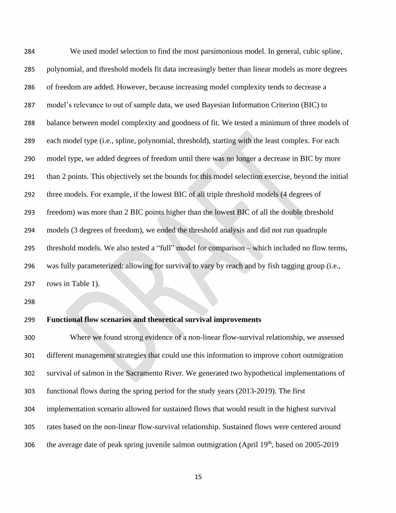
trials operated by USFWS Red Bluff Office, and the resulting expanded total catch numbers 323

represent the total number of fish passing the screw trap at Red Bluff. The rotary screw traps are 324

38 river kilometers upstream of the region of interest, and therefore approximately represents the 325

daily number of fish entering the region of interest during their outmigration. The screw traps are 326

operated continuously, except during the passage of significant numbers of hatchery fish or 327

during storm conditions (B. Poytress, UFSWS, pers. comm.). As a result, some spring sampling 328

days are missing from our study period. Furthermore, some days of significant hatchery fish 329

17

catches were also removed from the dataset; these days were identified as days when expanded 330

daily catch total surpassed 80,000 fish. 331

To estimate the realized water budget, we multiplied the sum of the mean daily flow 332

estimates (cfs) from March 15th to June 15th from the Keswick Dam gauge (USGS station 333

number 11370500) by 1.983x10-3 to convert to volume (TAF). To benefit outmigrating salmon, 334

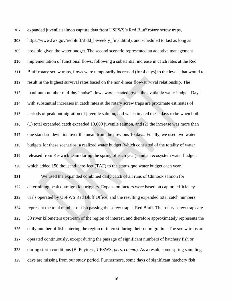
the non-linear flow-survival targets from the most parsimonious CJS model would need to be 335

realized at the Wilkins Slough gauge, so we estimated a daily net change between Keswick Dam 336

and Wilkins Slough. This approximates the net difference between water inputs (tributaries) and 337

water exports (water diversions) between the Keswick Dam and Wilkins Slough at a daily time 338

step. Finally, all functional flow implementation scenarios had three important regulatory 339

constraints: (1) minimum Keswick flows of 3,250 cfs (National Marine Fisheries Service 2009 340

Biological Opinion and Conference Opinion on the Long-Term Operations of the Central Valley 341

Project and State Water Project: NMFS 2009 BiOp), (2) maximum Keswick flow reduction rate 342

of 15% per day (U.S. Bureau of Reclamation 2008 Central Valley Project Biological 343

Assessment), and (3) no alteration to any daily Keswick releases that were deemed to be for flood 344

control (>20,000 cfs). 345

We then modeled the impact of the different flow implementation scenarios on cohort 346

outmigration survival of spring-outmigrating juvenile Chinook salmon. We used parametric 347

bootstrapping, where the pertinent logit-transformed survival distribution from the CJS model 348

(given flow levels at Wilkins Slough for that day) were resampled corresponding to the expanded 349

daily total catch at the Red Bluff screw traps. We estimated the mean logit-scale survival from 350

the totality of samples across all days of the spring-period, and then re-scaled (inverse-logit 351

transform). For missing daily values, we imputed catch using a linear interpolation of the time-352

18

series. Finally, to provide a baseline for assessing the potential survival gains of each scenario, 353

we estimated the cohort outmigration survival for the status-quo (using the observed spring 354

hydrograph in the years 2013-2019). 355

356

RESULTS 357

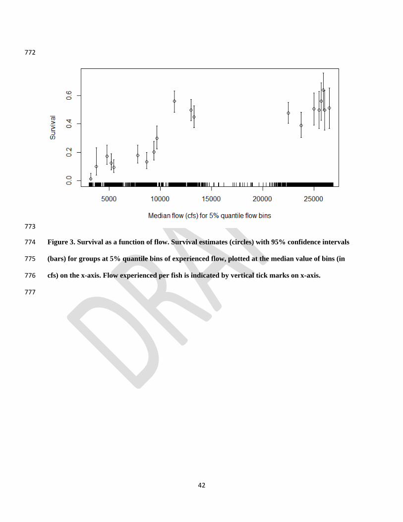
We found strong evidence of non-linearity in the flow-survival relationship (CJS model 358

with grouping based on 5% quantile flow bins, Fig. 3). Survival was positively related to flow 359

for values up to 10,000 cfs, followed by a sharp increase in survival near 10,000 cfs, at which 360

point survival asymptotes at approximately 50%. 361

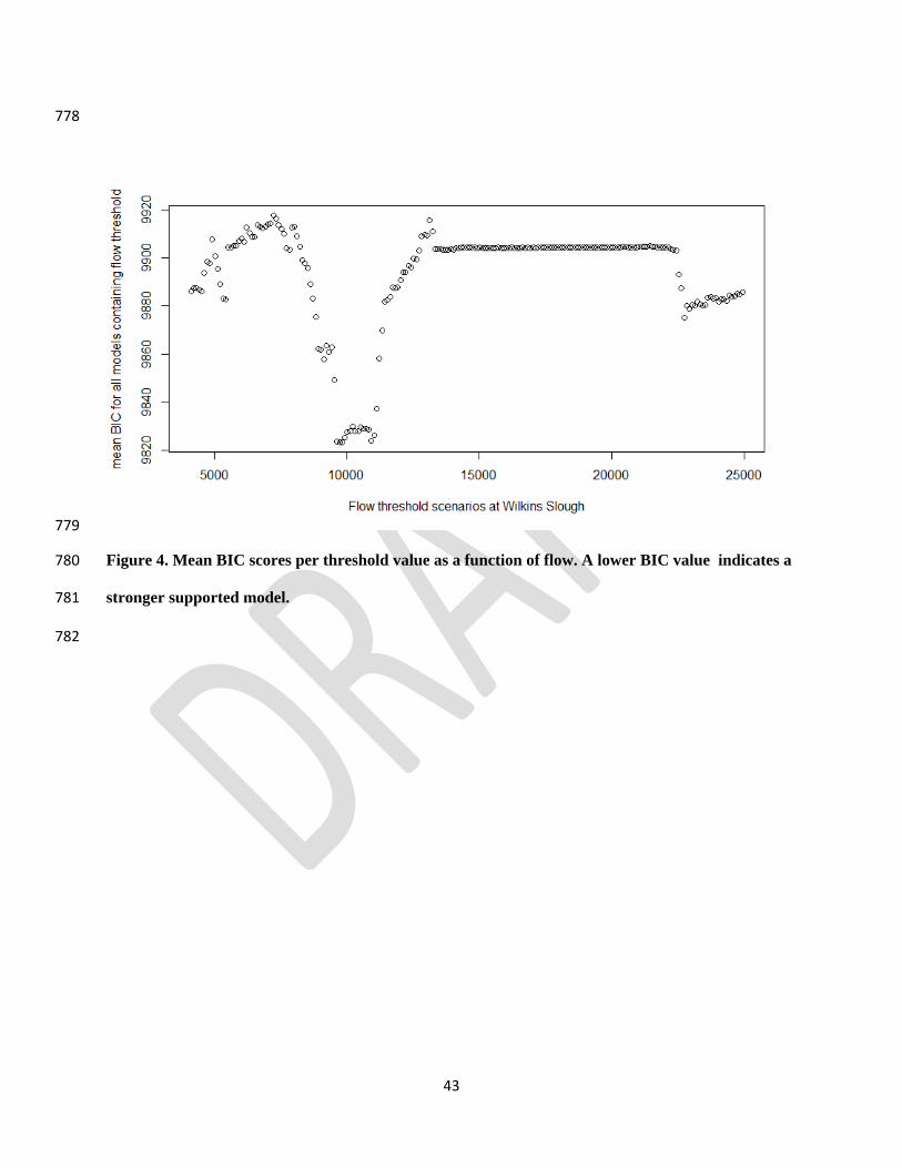
Out of 724,567 models we tested, the triple threshold models were the most 362

parsimonious, with 12 that were within 2 BIC points of the top model (Table S1). We estimated 363

survival parameters and threshold values (4,259, 10,712, and 22,872 cfs) from these 12 models 364

using model averaging. The threshold models were substantially better supported than any of the 365

other model types tested (∆BIC > 29). Furthermore, these threshold models, as well as all 366

polynomial and spline models, were better supported than the linear, log-linear, and full models 367

(∆BIC > 146), indicating strong support of a nonlinear flow-survival relationship. Full models 368

including fish length and origin (wild or hatchery) parameters did not increase parsimony, and 369

therefore these parameters were not included in flow survival models (Table S1). 370

In order to better understand model fit across the range of potential flow thresholds, for 371

each flow value tested in the threshold models, we estimated the mean BIC of all models that 372

included that flow value as one of its thresholds (Fig. 4). With similar results to the model 373

selection exercise, models with flow thresholds around 4,259, 10,712, and 22,872 cfs had strong 374

support (i.e., lower mean BIC). We labeled these “minimum” (4,259 cfs), “historic mean” 375

19

(10,712 cfs), and “high” (22,872 cfs). The historic mean threshold had highest support of the 376

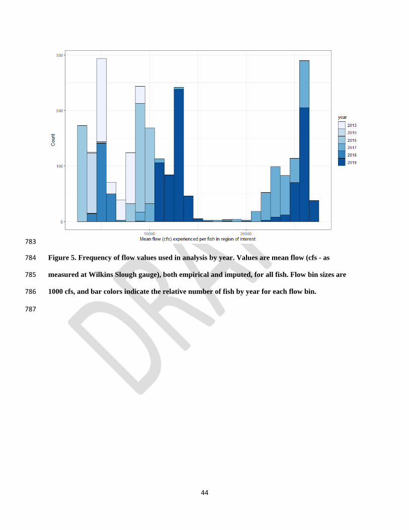
three thresholds (Fig. 4). Few fish experienced flow values between approximately 14,000 and 377

21,000 cfs (Fig. 5), and therefore model fit did not vary significantly with thresholds found in 378

this range. 379

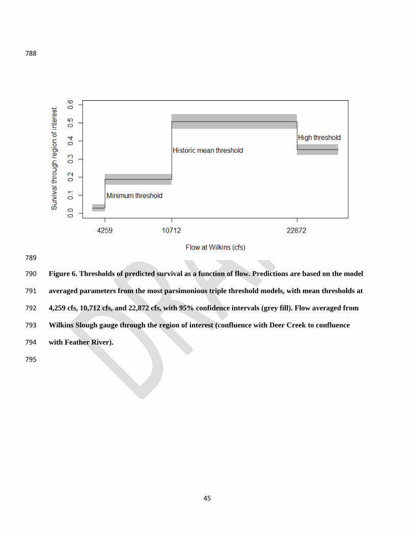
We used model averaged parameter estimates to predict survival for the range of flow 380

values (Fig. 6). There was a 6.3 fold increase in survival from flows below 4,259 cfs (0.03), to 381

flows between 4,259 and 10,712 cfs (0.189). There was a 2.7 fold increase in survival from flows 382

between 4,259 and 10,712 cfs, to flows above 10,712 cfs (0.508). Overall, there was a 16.9 fold 383

increase in survival from flow below 4,259, to flows above 10,712 cfs. Finally, survival 384

decreased above the 22,872 cfs threshold to 0.353. Survival was significantly different between 385

groups, with non-overlapping 95% confidence intervals. The 22,872 cfs threshold may be an 386

artifact of lower detection efficiencies associated with fish utilizing additional high flow 387

migration routes which have with less receiver coverage. 388

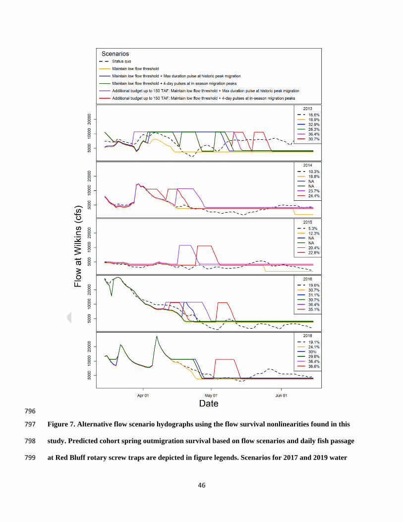
We compared modeled cohort outmigration survival rates among five different water 389

release scenarios for five water years with the modeled survival rates for actual flows (Fig. 7). 390

Water years 2013 (Dry), 2014 and 2015 (Critical), and 2016 and 2018 (Below Normal) represent 391

three classes of water supply scarcity in the Sacramento River Basin 392

(http://cdec.water.ca.gov/reportapp/javareports?name=WSIHIST). For Dry year 2013 and Below 393

Normal years 2016 and 2018, the three alternative scenarios using the available water budget 394

resulted in survival rate increases ranging from 55 to 98%, while the scenarios with an additional 395

150 TAF resulted in survival rates increases ranging from 79 to 119%. 396

For Critical years 2014 and 2015, the realized water budgets were not sufficient to allow 397

for the alternative release scenarios, beyond just maintaining flows above the low flow threshold 398

20

for as long as possible (resulting in survival rate increases of 83 and 132%, respectively). 399

Scenarios using an additional 150 TAF resulted in survival rate increases ranging from 130 to 400

330%. 401

402

DISCUSSION 403

Streamflow is a master variable in stream ecology, influencing biological and physical 404

habitat characteristics, and if not managed properly, flow alteration can be a serious threat to 405

freshwater ecosystems. Yet, water management decisions continue to be poorly informed by 406

environmental research (Davies et al, 2014; Horne et al., 2016). In the Sacramento River Basin, 407

surface water demands exceed supplies in all but the wettest years (Grantham and Viers, 2014), 408

and there is a pressing need to optimally allocate those limited resources to meet management 409

objectives, including ecosystem benefits. We identified threshold responses in salmon 410

outmigration survival across a range of observed instream flow rates. These relationships are 411

valuable tools for updating water management practices aimed at balancing competing demands. 412

Applying our minimum threshold (4,259 cfs) as a lower critical flow boundary for functional 413

flows could result in a 6.3 fold increase in outmigration survival. Flows above the historic mean 414

threshold (10,712 cfs) could provide an additional 2.7 fold increase in survival. This threshold 415

could be enacted when the resources are available, especially if coordinated with hatchery 416

releases or peak wild salmon migration periods. All else being equal, these survival gains could 417

result in concomitant increases in adult escapement. These modeled survival benefits justify the 418

need to identify ways to exceed these flow thresholds more consistently and for longer periods 419

during the spring months. 420

21

High flows promote favorable outmigration conditions for Chinook salmon juveniles, 421

resulting in increased survival to the ocean (Connor et al., 2003; Smith et al., 2003). We 422

identified an optimal threshold of 10,712 cfs, which we labeled historic mean, as it is similar to 423

the long-term average of natural spring flow conditions under which Chinook salmon have 424

evolved in this system (Fig. 1). Outmigrating juveniles move at higher speeds with higher flow 425

(Berggren and Filardo, 1993), limiting their exposure time to predators and other hazards. 426

Movement speeds and survival rates of wild Chinook salmon juveniles in this section of the river 427

are strongly correlated (Notch et al., 2020). Additionally, high flows typically increase water 428

turbidity, which may aid juveniles in evading predators (Gregory and Levings, 1998). Flow 429

levels above the historic mean threshold represent normal spring time flows under natural runoff 430

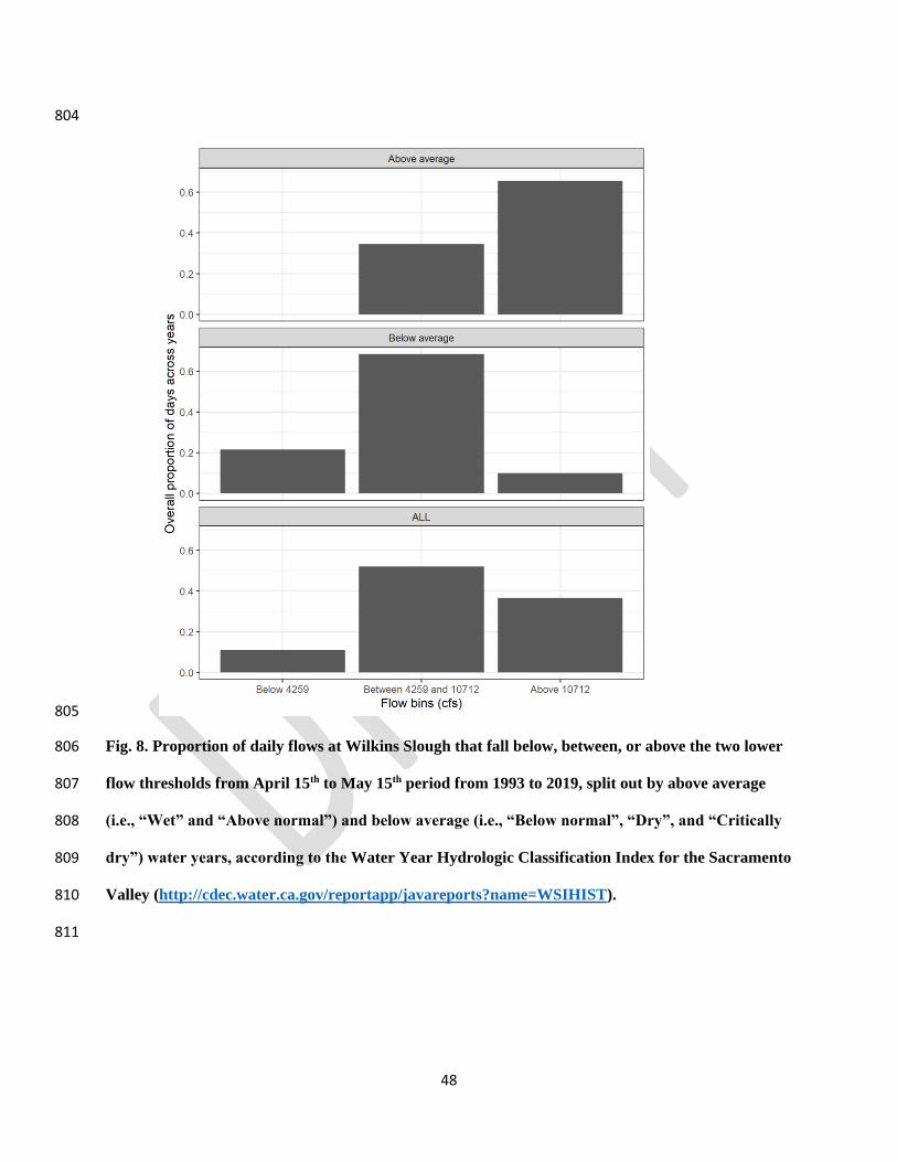
and streamflow conditions up until approximately May 15th (Fig. 1). Yet, from 1993 and 2019 431

such flows were only achieved in 37% of days during the April 15 – May 15 peak outmigration 432

period, and only 10% of days in below average water years (Fig. 8), and were even less likely to 433

occur later in the spring (Fig. 9). In late spring (after approximately April 15), tributary 434

accretions subside and demand for agricultural water deliveries increase dramatically, a 435

combination that creates progressively diminished instream flow in downstream reaches (Fig.1). 436

Sturrock et al. (2019) found that under current water management regimes, the low flows and 437

high water temperatures that occur in the late spring are selective forces against the later-438

migrating smolt juvenile life history type (>75mm fork length [FL]). Ultimately, the 439

implementation of ecologically functional flows above the 10,712 cfs threshold could be a 440

powerful tool to restore functional parts of the natural flow regime during critical periods of the 441

salmon life history. 442

22

The mechanism driving the lower flow threshold (4,259 cfs) is unclear. Anecdotal 443

observations indicate that under certain low flow conditions, sections of the Sacramento River 444

may have increased habitat heterogeneity, in particular with regards to pools and riffles where 445

predator ambush habitat is likely created (Michel, pers. obs.). Flow influences other important 446

environmental variables, such as water temperature, that might also have nonlinear relationships 447

with survival. Because temperature and flow are highly correlated (flow and temperature 448

experienced for these fish as measured at Wilkins Slough had a Pearson’s correlation coefficient 449

of 0.93) and flow is the most persistent driver of survival in the CCV (Henderson et al., 2019, 450

Notch et al., 2020), we did not include temperature in this analysis. At very low flows during the 451

latter end of the spring period, water temperature in the lower Sacramento River can approach 452

the thermal tolerance of juvenile Chinook salmon. Under the lower flow threshold conditions, 453

mean water temperature was 19.9º C (0.5 SD) at the Wilkins Slough gauge. At this temperature, 454

salmon health and vulnerability to predation can be affected and ultimately lead to lowered 455

survival (Lehman et al., 2017, Marine et al., 2004, Michel et al., 2020, Miller et al., 2014). 456

During most years, spring outmigration flows are above the lower threshold, and these 457

unfavorable conditions are usually only observed during years of drought (e.g., 1994, 2013-2015; 458

Fig. 9). However, in recent years, spring flows below this lower threshold have occurred in years 459

of near average precipitation (i.e. 2016, 2018; Fig. 9), likely resulting from a complex suite of 460

factors, including reservoir management strategies for conserving cold water for endangered 461

winter-run Chinook salmon, and increasing water deliveries for out of stream uses during the 462

summer months. 463

Of the models we tested, the threshold models had strongest support, possibly because 464

they allow for a sharp transition between survival levels as a result of a small changes in flow 465

23

across some ecologically important value. For example, exceeding a given threshold can lead to 466

river bank overflow, which activates seasonal floodplains, providing juvenile salmon an 467

alternative downstream migration route. This is the hypothesized mechanism for the high 468

threshold (22,872 cfs): Tisdale Weir, within the area of interest, overtops at approximately this 469

flow value, allowing fish to enter the Sutter Bypass. Survival decreased at flows above this 470

threshold, suggesting that fish utilizing this alternate route experienced decreased survival 471

compared to fish remaining in the Sacramento River. While flood bypasses are generally 472

considered to be high quality rearing habitat for juvenile salmon (Sommer et al., 2001), there is 473

little known about the relative survival of fish utilizing these habitats. The detection efficiency of 474

fish utilizing the bypass route is likely lower, however, which could be a confounding driver of 475

the high threshold. 476

The modeled functional flow scenarios indicated that substantial gains over the status quo 477

were possible by leveraging the thresholds we identified. These flow scenarios lead to increases 478

in annual outmigration survival ranging between 57% and 130% without additions to the water 479

budget, and increases ranging from 79% to 330% with a modest 150 TAF addition to the water 480

budget (Fig. 7). There were no clear and consistent differences in survival between the historic 481

peak migration pulse flow scenario and the 4-day adaptive pulse flow scenario, whether with the 482

realized water budget or with the additional environmental water budget. We included an 483

additional scenario where flows mimicked the status quo hydrograph, but flows were not 484

allowed to dip below the minimum threshold, which alone led to substantial gains in survival in 485

the Critical Dry water years 2014 and 2015 (Fig. 7). Adaptive functional flow scenarios may be 486

preferable to a single-pulse, fixed calendar date scenario in ways not measured in this study. For 487

24

example, the adaptive implementation will be more responsive to hydrologic or biotic nuances of 488

a given year, and promote more diversity in outmigration timing. 489

Our analysis is consistent with many studies concluding that flow is a strong driver for 490

Chinook salmon smolt spring outmigration survival. This period of time coincides with peak 491

hatchery releases and peak natural-origin outmigration of fall-run Chinook salmon, the stock that 492

supports an important commercial and recreational fishery, as well as peak outmigration of ESA 493

threatened wild spring-run Chinook salmon smolts from Sacramento River tributaries. Spring-494

run Chinook salmon populations spawn at high elevations and therefore experience slower 495

growth rates and delayed outmigration timing compared to other Chinook salmon populations 496

spawning in the rivers on the valley floor, making them particularly vulnerable to late spring low 497

flows. Further, these late outmigrants are subject to asynchronous flow conditions between natal 498

streams (when their initial downstream migration is triggered by snow melt or spring freshets in 499

the tributary) and the mainstem Sacramento River, where they experience periods of low 500

managed flows. Restoring the functionality of the spring flow regime during wild smolt 501

outmigration is a critical step towards promoting sustainable fisheries (Jager and Rose, 2003), as 502

well as restoring a threatened population of salmon. 503

Other CCV native fish species may require different flow conditions during the spring, 504

potentially creating water management conflicts. For example, high flows and cold water from 505

dam releases may have detrimental impacts on threatened green sturgeon (Acipenser medirostris) 506

in the Sacramento River (Zarri et al., 2019). Similarly, endangered winter-run Chinook salmon 507

rely on cold water released from Shasta Reservoir during egg development in the summer, which 508

is contingent on water operations that allow sufficient cold water availability in Shasta Reservoir 509

for the summer months (Martin et al., 2017). Increasing spring flows for the benefit of fall-run 510

25

and threatened spring-run Chinook salmon requires carefully balancing the needs of other 511

protected species in the Sacramento River. 512

Our study focused on the flow-survival relationship for the smolt outmigration life-513

history, as it was based on acoustically tagged fish, and tag size constraints precluding the 514

tagging of smaller juveniles. However, other juvenile life-history types, namely fry and parr 515

(approximately <55mm, and 55 to 75mm FL, respectively), are important contributors to CCV 516

Chinook salmon populations (Sturrock et al., 2019). While higher winter and spring flows also 517

benefit fry and parr life histories (Sturrock et al., 2015, 2019) the flow thresholds defined in this 518

study are for smolt outmigration and are likely not directly compatible with fry and parr life 519

histories, which need flows appropriate for rearing. In general, targeting ecologically functional 520

flows that mimic the shape of the historic hydrograph under which these fish evolved should also 521

benefit these other life histories and promote life history diversity. 522

Our study identifies key thresholds in the flow-survival relationships that can help water 523

and fisheries managers evaluate trade-offs associated with different water management options 524

that are, by law, supposed to balance in-stream and out-of-stream management objectives. We 525

recommend that future studies attempt flow experiments to verify that migrating salmon would 526

benefit as predicted from managed flow augmentation (such as pulse flows). It is likely that such 527

pulse flows will engendered larger survival gains than predicted here: flow pulses are known to 528

promote juvenile Chinook salmon to initiate their downstream migration (Sykes et al., 2009), 529

allowing a larger portion of the population to take advantage of the associated improvements in 530

survival. Courter et al. (2016) used managed flow releases in the Yakima River, Washington, to 531

show the positive impact of increased flow on Chinook salmon smolt survival, which was then 532

used to implement a minimum flow target. Experimental pulse flows may also help decouple the 533

26

mechanisms driving increased survival, because increased flows through reservoir releases may 534

not affect temperature and turbidity the same as storm-related flow increases. Ultimately, 535

functional flows in CCV should include a spring pulse flow component that mimics the 536

characteristics of spring freshets and snowmelt events of a natural hydrograph. These will benefit 537

outmigrating smolts and also engender many other benefits to the ecosystem (Kiernan et al., 538

2012, Poff et al., 1997). 539

This is timely research as the frequency of drought events is predicted to increase in the 540

CCV, creating additional stress to already vulnerable salmon populations (Yates et al., 2008). 541

Munsch et al. (2019) showed a truncation of fish size and outmigration timing of juvenile 542

Chinook salmon from the Sacramento River during warmer springs, which could lead to lower 543

ocean survival. This highlights the influence of climate change on salmon species phenology and 544

dynamics and the need for new flow management policies that include the potential impacts of 545

future climate warming. In the Sacramento River, finding functional flows that could simulate 546

ecologically critical aspects of the natural spring hydrograph, especially in increasingly common 547

dry water years, is a critical step in ensuring the resiliency of juvenile Chinook salmon and other 548

native fish species into the 21st century. 549

550

27

ACKNOWLEDGEMENTS 551

We thank Cramer Fish Sciences, NOAA Fisheries, and US Fish and Wildlife Service (USFWS) 552

for providing portions of the tagging data used here. Funding and resources were provided by the 553

US Bureau of Reclamation, U.S Fish and Wildlife Service’s Anadromous Fish Restoration 554

Program, and the Central Valley Project Improvement Act. Wild and hatchery fish collection 555

was made possible by staff and support from USFWS - Red Bluff Fish and Wildlife Office and 556

the California Department of Fish and Wildlife Red Bluff Office. Material, administrative, and 557

logistical support was provided by Arnold Ammann and the National Marine Fisheries Service - 558

Southwest Fisheries Science Center. We thank Carlos Garza and the Molecular Ecology Team 559

for genetic assignment of tagged wild fish. Finally, we thank Nate Mantua, Steve Zeug, and 560

Michael Beakes for insightful reviews of the manuscript. All fish were handled humanely 561

according to the methods described in NOAA IACUC permit # DANNE1905. The data that 562

support the findings of this study are openly available from the National Oceanic and 563

Atmospheric Administration’s ERDDAP data server at 564

https://oceanview.pfeg.noaa.gov/erddap/tabledap/FED_JSATS_detects.html. The authors report 565

no conflict of interest. 566

567

28

REFERENCES 568

Arthington, A. H., A. Bhaduri, S. E. Bunn, S. E. Jackson, R. E. Tharme, D. Tickner, B. Young, 569

M. Acreman, N. Baker, S. Capon, A. C. Horne, E. Kendy, M. E. McClain, N. L. Poff, B. 570

D. Richter, and S. Ward. 2018. The Brisbane Declaration and Global Action Agenda on 571

Environmental Flows. Frontiers in Environmental Science 6. 572

Berggren, T. J., and M. J. Filardo. 1993. An Analysis of Variables Influencing the Migration of 573

Juvenile Salmonids in the Columbia River Basin. North American Journal of Fisheries 574

Management 13:48-63. 575

Brown, L. R., and M. L. Bauer. 2009. Effects of hydrologic infrastructure on flow regimes of 576

California's Central Valley rivers: Implications for fish populations. River Research and 577

Applications 26:751-765. 578

Bunn, S. E., and A. H. Arthington. 2002. Basic Principles and Ecological Consequences of 579

Altered Flow Regimes for Aquatic Biodiversity. Environmental Management 30:492-580

507. 581

Clemento, A. J., A. Abadia-Cardoso, H. A. Starks, and J. C. Garza. 2011. Discovery and 582

characterization of single nucleotide polymorphisms in Chinook salmon, Oncorhynchus 583

tshawytscha. Molecular Ecology Resources 11:50-66. 584

Connor, W. P., H. L. Burge, J. R. Yearsley, and T. C. Bjornn. 2003. Influence of Flow and 585

Temperature on Survival of Wild Subyearling Fall Chinook Salmon in the Snake River. 586

North American Journal of Fisheries Management 23:362-375. 587

Cordoleani, F., J. Notch, A. McHuron, A. J. Ammann, and C. J. Michel. 2018. Movement and 588

Survival of Wild Chinook Salmon Smolts from Butte Creek During Their Out‐Migration 589

29

to the Ocean: Comparison of a Dry Year versus a Wet Year. Transactions of the 590

American Fisheries Society 147:171-184. 591

Courter, I. I., T. M. Garrison, T. J. Kock, R. W. Perry, D. B. Child, and J. D. Hubble. 2016. 592

Benefits of Prescribed Flows for Salmon Smolt Survival Enhancement Vary 593

Longitudinally in a Highly Managed River System. River Research and Applications 594

32:1999-2008. 595

Deters, K. A., R. S. Brown, K. M. Carter, J. W. Boyd, M. B. Eppard, and A. G. Seaburg. 2010. 596

Performance Assessment of Suture Type, Water Temperature, and Surgeon Skill in 597

Juvenile Chinook Salmon Surgically Implanted with Acoustic Transmitters. Transactions 598

of the American Fisheries Society 139:888-899. 599

Fisher, F. W. 1994. Past and present status of Central Valley Chinook Salmon. Conservation 600

Biology 8:870-873. 601

Grantham, T. E., and J. H. Viers. 2014. 100 years of California’s water rights system: patterns, 602

trends and uncertainty. Environmental Research Letters 9:084012. 603

Gregory, R. S., and C. D. Levings. 1998. Turbidity reduces predation on migrating juvenile 604

Pacific salmon. Transactions of the American Fisheries Society 127:275-285. 605

Hanak, E., and J. R. Lund. 2012. Adapting California’s water management to climate change. 606

Climatic Change 111:17-44. 607

Henderson, M. J., I. S. Iglesias, C. J. Michel, A. J. Ammann, and D. D. Huff. 2019. Estimating 608

spatial–temporal differences in Chinook salmon outmigration survival with habitat- and 609

predation-related covariates. Canadian Journal of Fisheries and Aquatic Sciences 610

76:1549-1561. 611

30

Horne, A., J. M. Szemis, S. Kaur, J. A. Webb, M. J. Stewardson, A. Costa, and N. Boland. 2016. 612

Optimization tools for environmental water decisions: A review of strengths, weaknesses, 613

and opportunities to improve adoption. Environmental Modelling & Software 84:326-614

338. 615

Huber, E. R., and S. M. Carlson. 2015. Temporal Trends in Hatchery Releases of Fall-Run 616

Chinook Salmon in California's Central Valley. San Francisco Estuary and Watershed 617

Science, 13(2). 618

Hunsicker, M. E., C. V. Kappel, K. A. Selkoe, B. S. Halpern, C. Scarborough, L. Mease, and A. 619

Amrhein. 2016. Characterizing driver–response relationships in marine pelagic 620

ecosystems for improved ocean management. Ecological Applications 26:651-663. 621

Jager, H. I., and K. A. Rose. 2003. Designing Optimal Flow Patterns for Fall Chinook Salmon in 622

a Central Valley, California, River. North American Journal of Fisheries Management 623

23:1-21. 624

Kiernan, J. D., P. B. Moyle, and P. K. Crain. 2012. Restoring native fish assemblages to a 625

regulated California stream using the natural flow regime concept. Ecological 626

Applications 22:1472-1482. 627

Kimmerer, W. J. 2008. Losses of Sacramento River Chinook salmon and delta smelt to 628

entrainment in water diversions in the Sacramento–San Joaquin Delta. San Francisco 629

Estuary and Watershed Science, 6(2). 630

Kjelson, M., P. F. Raquel, and F. W. Fisher. 1981. Influences of freshwater inflow on chinook 631

salmon (Oncorhynchus tshawystcha) in the Sacramento-San Joaquin Estuary. Pages 88-632

108 in Proceedings of the National Symposium on Freshwater Inflow to Estuaries. U.S. 633

Fish and Wildlife Service. 634

31

Laake, J. L. 2013. RMark: An R Interface for Analysis of Capture-Recapture Data with MARK. 635

AFSC Processed Rep 2013-01, 25p. Alaska Fish. Sci. Cent., NOAA, Natl. Mar. Fish. 636

Serv., 7600 Sand Point Way NE, Seattle WA 98115. 637

Lebreton, J.-D., K. P. Burnham, J. Clobert, and D. R. Anderson. 1992. Modeling Survival and 638

Testing Biological Hypotheses Using Marked Animals: A Unified Approach with Case 639

Studies. Ecological Monographs 62:67-118. 640

Lehman, B., D. D. Huff, S. A. Hayes, and S. T. Lindley. 2017. Relationships between Chinook 641

salmon swimming performance and water quality in the San Joaquin River, California. 642

Transactions of the American Fisheries Society 146:349-358. 643

Marine, K. R., and J. J. Cech. 2004. Effects of High Water Temperature on Growth, 644

Smoltification, and Predator Avoidance in Juvenile Sacramento RiverChinook Salmon. 645

North American Journal of Fisheries Management 24:198-210. 646

Martin, B. T., A. Pike, S. N. John, N. Hamda, J. Roberts, S. T. Lindley, and E. M. Danner. 2017. 647

Phenomenological vs. biophysical models of thermal stress in aquatic eggs. Ecology 648

Letters 20:50-59. 649

McMichael, G. A., M. B. Eppard, T. J. Carlson, J. A. Carter, B. D. Ebberts, R. S. Brown, M. 650

Weiland, G. R. Ploskey, R. A. Harnish, and Z. D. Deng. 2010. The Juvenile Salmon 651

Acoustic Telemetry System: A New Tool. Fisheries 35:9-22. 652

Michel, C. J., A. J. Ammann, S. T. Lindley, P. T. Sandstrom, E. D. Chapman, M. J. Thomas, G. 653

P. Singer, A. P. Klimley, and R. B. MacFarlane. 2015. Chinook salmon outmigration 654

survival in wet and dry years in California’s Sacramento River. Canadian Journal of 655

Fisheries and Aquatic Sciences 72:1749-1759. 656

32

Michel, C. J. 2019. Decoupling outmigration from marine survival indicates outsized influence 657

of streamflow on cohort success for California’s Chinook salmon populations. Canadian 658

Journal of Fisheries and Aquatic Sciences 76:1398-1410. 659

Michel, C. J., M. J. Henderson, C. M. Loomis, J. M. Smith, N. J. Demetras, I. S. Iglesias, B. M. 660

Lehman, and D. D. Huff. 2020. Fish predation on a landscape scale. Ecosphere 661

11:e03168. 662

Miller, K. M., A. Teffer, S. Tucker, S. R. Li, A. D. Schulze, M. Trudel, F. Juanes, A. Tabata, K. 663

H. Kaukinen, N. G. Ginther, T. J. Ming, S. J. Cooke, J. M. Hipfner, D. A. Patterson, and 664

S. G. Hinch. 2014. Infectious disease, shifting climates, and opportunistic predators: 665

cumulative factors potentially impacting wild salmon declines. Evolutionary Applications 666

7:812-855. 667

Mount, J., B. Gray, K. Bork, J. Cloern, F. Davis, T. Grantham, L. Grenier, J. Harder, Y. 668

Kuwayama, P. Moyle, M. Schwartz, A. Whipple, and S. Yarnell. 2019. A Path Forward 669

for California's Freshwater Ecosystems. Public Policy Institute of California. 670

Munsch, S. H., C. M. Greene, R. C. Johnson, W. H. Satterthwaite, H. Imaki, and P. L. Brandes. 671

2019. Warm, dry winters truncate timing and size distribution of seaward-migrating 672

salmon across a large, regulated watershed. Ecological Applications 29:e01880. 673

Munsch, S. H., K. S. Andrews, L. G. Crozier, R. Fonner, J. L. Gosselin, C. M. Greene, C. J. 674

Harvey, J. I. Lundin, G. R. Pess, J. F. Samhouri, and W. H. Satterthwaite. In review. 675

Potential for ecological nonlinearities and thresholds to inform Pacific salmon 676

management 677

Notch, J. J., A. S. McHuron, C. J. Michel, F. Cordoleani, M. Johnson, M. J. Henderson, and A. J. 678

Ammann. 2020. Outmigration survival of wild Chinook salmon smolts through the 679

33

Sacramento River during historic drought and high water conditions. Environmental 680

Biology of Fishes. 681

Palmer, M. A., C. A. Reidy Liermann, C. Nilsson, M. Flörke, J. Alcamo, P. S. Lake, and N. 682

Bond. 2008. Climate change and the world's river basins: anticipating management 683

options. Frontiers in Ecology and the Environment 6:81-89. 684

Petts, G. E. 2009. Instream Flow Science For Sustainable River Management. JAWRA Journal 685

of the American Water Resources Association 45:1071-1086. 686

Poff, N. L., J. D. Allan, M. B. Bain, J. R. Karr, K. L. Prestegaard, B. D. Richter, R. E. Sparks, 687

and J. C. Stromberg. 1997. The Natural Flow Regime. BioScience 47:769-784. 688

Pringle, C. M., M. C. Freeman, and B. J. Freeman. 2000. Regional effects of hydrologic 689

alterations on riverine macrobiota in the New World: tropical–temperate comparisons. 690

Bioscience 50: 807–823. 691

R Core Team. 2019. R: A language and environment for statistical computing. R Foundation for 692

Statistical Computing, Vienna, Austria. URL https://www.R-project.org/. 693

Rosenfeld, J. S. 2017. Developing flow–ecology relationships: Implications of nonlinear 694

biological responses for water management. Freshwater Biology 62(8):1305-1324. 695

Scheffer, M., S. Carpenter, J. A. Foley, C. Folke, and B. Walker. 2001. Catastrophic shifts in 696

ecosystems. Nature 413:591–596. 697

Smith, S. G., W. D. Muir, E. E. Hockersmith, R. W. Zabel, R. J. Graves, C. V. Ross, W. P. 698

Connor, and B. D. Arnsberg. 2003. Influence of river conditions on survival and travel 699

34

time of Snake River subyearling fall chinook salmon. North American Journal of 700

Fisheries Management 23:939-961. 701

Sommer, T. R., M. L. Nobriga, W. C. Harrell, W. Batham, and W. J. Kimmerer. 2001. 702

Floodplain rearing of juvenile chinook salmon: evidence of enhanced growth and 703

survival. Canadian Journal of Fisheries and Aquatic Sciences 58:325-333. 704

Speir, C., A. Mamula, and D. Ladd. 2015. Effects of Water Supply on Labor Demand and 705

Agricultural Production in California's San Joaquin Valley. Water Economics and Policy 706

1(2):1550003. 707

Sturrock, A. M., J. D. Wikert, T. Heyne, C. Mesick, A. E. Hubbard, T. M. Hinkelman, P. K. 708

Weber, G. E. Whitman, J. J. Glessner, and R. C. Johnson. 2015. Reconstructing the 709

Migratory Behavior and Long-Term Survivorship of Juvenile Chinook Salmon under 710

Contrasting Hydrologic Regimes. PLoS One 10:e0122380. 711

Sturrock, A. M., S. M. Carlson, J. D. Wikert, T. Heyne, S. Nusslé, J. E. Merz, H. J. W. Sturrock, 712

and R. C. Johnson. 2019. Unnatural selection of salmon life histories in a modified 713

riverscape. Global Change Biology 00:1-13. 714

Sykes, G. E., C. J. Johnson, and J. M. Shrimpton. 2009. Temperature and Flow Effects on 715

Migration Timing of Chinook Salmon Smolts. Transactions of the American Fisheries 716

Society 138:1252-1265. 717

Tanaka, S. K., T. Zhu, J. R. Lund, R. E. Howitt, M. W. Jenkins, M. A. Pulido, M. Tauber, R. S. 718

Ritzema, and I. C. Ferreira. 2006. Climate Warming and Water Management Adaptation 719

for California. Climatic Change 76:361-387. 720

35

White, G. C., and K. P. Burnham. 1999. Program MARK: survival estimation from populations 721

of marked animals. Bird Study 46:120-139. 722

Yarnell, S. M., J. H. Viers, and J. F. Mount. 2010. Ecology and Management of the Spring 723

Snowmelt Recession. BioScience. 60: 114-127. 724

Yarnell, S. M., G. E. Petts, J. C. Schmidt, A. A. Whipple, E. E. Beller, C. N. Dahm, P. Goodwin, 725

and J. H. Viers. 2015. Functional Flows in Modified Riverscapes: Hydrographs, Habitats 726

and Opportunities. BioScience 65:963-972. 727

Yarnell, S. M., E. D. Stein, J. A. Webb, T. Grantham, R. A. Lusardi, J. Zimmerman, R. A. Peek, 728

B. A. Lane, J. Howard, and S. Sandoval-Solis. 2020. A functional flows approach to 729

selecting ecologically relevant flow metrics for environmental flow applications. River 730

Research and Applications 36:318-324. 731

Yates, D., H. Galbraith, D. Purkey, A. Huber-Lee, J. Sieber, J. West, S. Herrod-Julius, and B. 732

Joyce. 2008. Climate warming, water storage, and Chinook salmon in California's 733

Sacramento Valley. Climatic Change 91:335-350. 734

Yoshiyama, R. M., F. W. Fisher, and P. B. Moyle. 1998. Historical abundance and decline of 735

Chinook Salmon in the Central Valley region of California. North American Journal of 736

Fisheries Management 18:487-521. 737

Zarri, L. J., E. M. Danner, M. E. Daniels, and E. P. Palkovacs. 2019. Managing hydropower dam 738

releases for water users and imperiled fishes with contrasting thermal habitat 739

requirements. Journal of Applied Ecology 56:2423-2430. 740

36

Table 1. Wild and hatchery tagged fish groups included in our analysis from 2013 to 2019. Release 741

locations are further described in Fig. 2. Genetic population assignments made using protocols 742

outlined in Clemento et al. (2011). 743

Population Origin Year Release Dates

Release

Location

N Genetic Population Origin

Mill Creek Wild 2013

Mid-April to

mid-May

MCRT 48

74% CCV fall-run

26% CCV spring-run

Coleman Hatchery 2013 Mid-April CNFH 285 100% CCV fall-run

Mill Creek Wild 2015

Mid-April to

mid-May

MCRT 110

44% CCV fall-run

56% CCV spring-run

Coleman Hatchery 2016

Early-April to

late-April

CNFH 540 100% CCV fall-run

Mill Creek Wild 2017

Mid-April to

late-April

MCRT 24 100% CCV fall-run

Coleman Hatchery 2017

Early-April to

late-April

CNFH 370 100% CCV fall-run

Sacramento River Wild† 2017 June 6 RBDD 33 100% CCV fall-run

Sacramento River Wild† 2018

Early-May to

early-June

RBDD 207 100% CCV fall-run

Livingston Stone Hatchery 2019 March 26 NFBC 199 100% Sacramento winter-run

Coleman Hatchery 2019 April 11 CNFH 140 100% CCV fall-run

Coleman Hatchery 2019 Late-May RBDD 480 100% CCV fall-run

TOTAL 2013-2019

Late-March

to early-June

2436

37

†Fish captured in rotary screw traps in the Sacramento River and tagged were assumed to be wild, although some 744

hatchery fish may have been misidentified and incidentally tagged. 745

746

38

747

748

Fig. 1. Mean daily Sacramento River hydrographs for the spring period from 2000-2019, excluding 749

those classified as wet (2006, 2011, 2017, 2019: 750

http://cdec.water.ca.gov/reportapp/javareports?name=WSIHIST), mean daily natural hydrograph 751

(dashed line), and mean daily expanded juvenile salmon passage (primarily natural-origin) (grey 752

points, data from USFWS Red Bluff rotary screw traps, 38 km upstream of the region of interest). 753

Flow levels (in cfs) are plotted through time at several gauges along the river, starting from 754

Keswick gauge (“dam release”: USGS station number 11370500) on the upstream end to Wilkins 755

Slough gauge (USGS station number 11390500) on the downstream end (color legend inset has 756

gauges listed in order from upstream to downstream). The mean daily natural flow regime is the 757

sum of the “full natural flow” statistic on the California Data Exchange Center 758

(http://cdec.water.ca.gov) for the Bend Bridge (BND) gauging station, along with the daily flow 759

from Mill Creek (USGS 11381500) and Deer Creek (USGS 11383500) gauges, both located 760

upstream of major diversions. It is therefore representative of the estimated full natural flow 761

entering the region of interest. A 10-day moving average smoothing has been applied to all 762

39

hydrographs and fish passage data. All stream gauges are operated by either USGS, US Bureau of 763

Reclamation, or California Department of Water Resources. 764

765

40

766

Fig. 2. Study area, release locations, and receiver locations. Region of interest spans from the 767

confluence with Deer Creek to the confluence with Feather River. Release location abbreviations 768

41

are: CNFH: Coleman National Fish Hatchery, NFBC: North Fork Battle Creek, RBDD: Red Bluff 769

Diversion Dam, MCRT: Mill Creek rotary screw trap. 770

771

42

772

773

Figure 3. Survival as a function of flow. Survival estimates (circles) with 95% confidence intervals 774

(bars) for groups at 5% quantile bins of experienced flow, plotted at the median value of bins (in 775

cfs) on the x-axis. Flow experienced per fish is indicated by vertical tick marks on x-axis. 776

777

43

778

779

Figure 4. Mean BIC scores per threshold value as a function of flow. A lower BIC value indicates a 780

stronger supported model. 781

782

44

783

Figure 5. Frequency of flow values used in analysis by year. Values are mean flow (cfs - as 784

measured at Wilkins Slough gauge), both empirical and imputed, for all fish. Flow bin sizes are 785

1000 cfs, and bar colors indicate the relative number of fish by year for each flow bin. 786

787

45

788

789

Figure 6. Thresholds of predicted survival as a function of flow. Predictions are based on the model 790

averaged parameters from the most parsimonious triple threshold models, with mean thresholds at 791

4,259 cfs, 10,712 cfs, and 22,872 cfs, with 95% confidence intervals (grey fill). Flow averaged from 792

Wilkins Slough gauge through the region of interest (confluence with Deer Creek to confluence 793

with Feather River). 794

795

46

796

Figure 7. Alternative flow scenario hydographs using the flow survival nonlinearities found in this 797

study. Predicted cohort spring outmigration survival based on flow scenarios and daily fish passage 798

at Red Bluff rotary screw traps are depicted in figure legends. Scenarios for 2017 and 2019 water 799

47

years are not depicted, as wet conditions in those years precluded the need for functional flows. In 800

the critically dry years of 2014 and 2015, functional flows were not possible based on actual water 801

budget (“NA” for respective survival estimates in legend). 802

803

48

804

805

Fig. 8. Proportion of daily flows at Wilkins Slough that fall below, between, or above the two lower 806

flow thresholds from April 15th to May 15th period from 1993 to 2019, split out by above average 807

(i.e., “Wet” and “Above normal”) and below average (i.e., “Below normal”, “Dry”, and “Critically 808

dry”) water years, according to the Water Year Hydrologic Classification Index for the Sacramento 809

Valley (http://cdec.water.ca.gov/reportapp/javareports?name=WSIHIST). 810

811

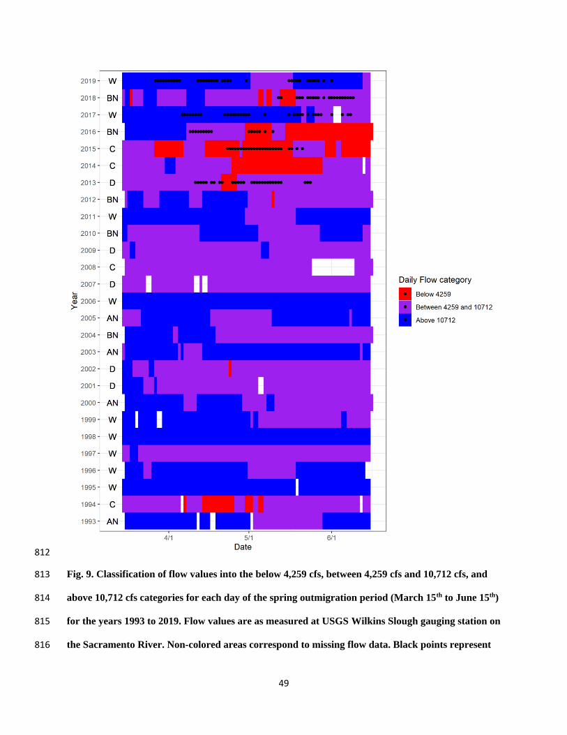
49

812

Fig. 9. Classification of flow values into the below 4,259 cfs, between 4,259 cfs and 10,712 cfs, and 813

above 10,712 cfs categories for each day of the spring outmigration period (March 15th to June 15th) 814

for the years 1993 to 2019. Flow values are as measured at USGS Wilkins Slough gauging station on 815

the Sacramento River. Non-colored areas correspond to missing flow data. Black points represent 816

50

days when acoustic tagged fish were entering the region of interest. Text within box indicates the 817

Water Year Hydrologic Classification Index for the Sacramento Valley 818

(http://cdec.water.ca.gov/reportapp/javareports?name=WSIHIST); year type codes are W – wet, 819

AN – above normal, BN, below normal, D – dry, and C – critically dry. 820