Embed Size (px)
Citation preview

1
Dynamic Programming
Jose RolimUniversity of Geneva
Dynamic Programming Jose Rolim 2
All pair shortest path
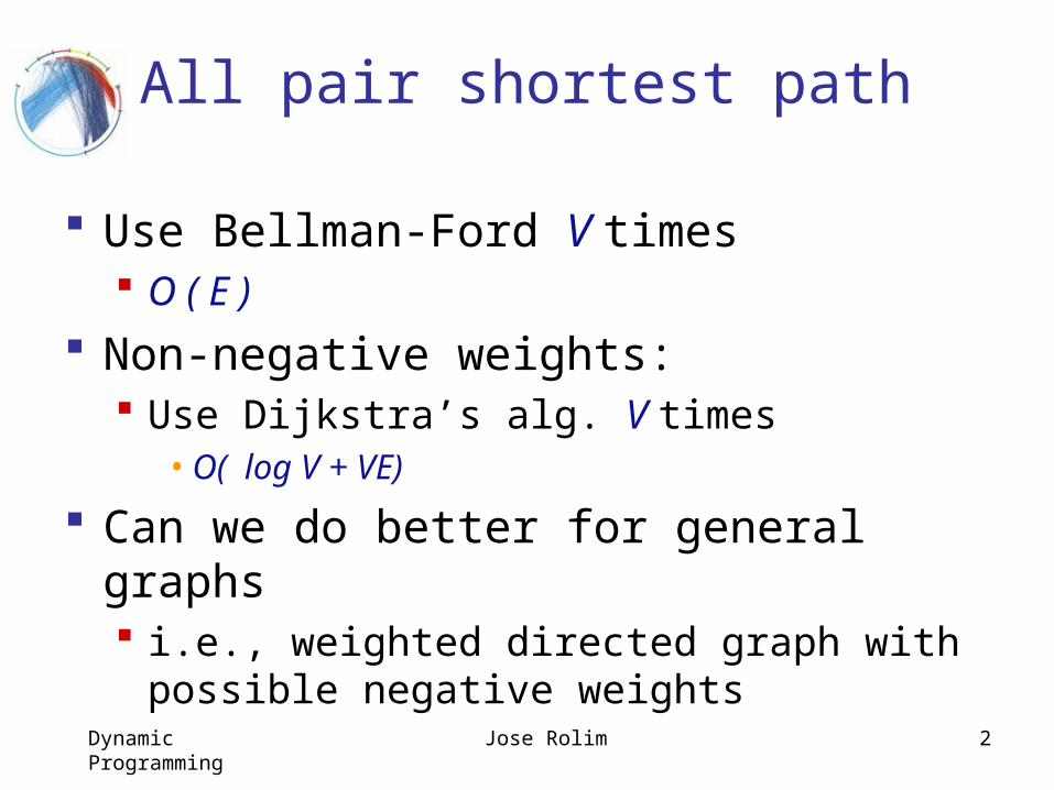
Use Bellman-Ford V times O ( E )
Non-negative weights: Use Dijkstra’s alg. V times
• O( log V + VE)
Can we do better for general graphs i.e., weighted directed graph with
possible negative weights
Dynamic Programming Jose Rolim 3
Terminologies
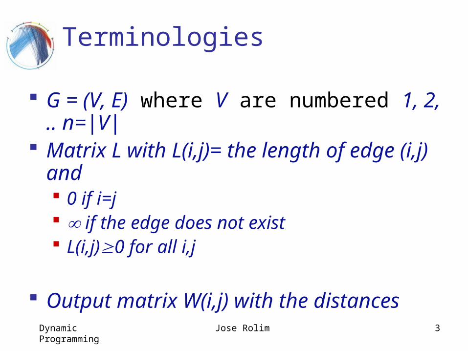
G = (V, E) where V are numbered 1, 2, .. n=|V|
Matrix L with L(i,j)= the length of edge (i,j) and 0 if i=j if the edge does not exist L(i,j)0 for all i,j
Output matrix W(i,j) with the distances
Dynamic Programming Jose Rolim 4
Dynamic programming approach
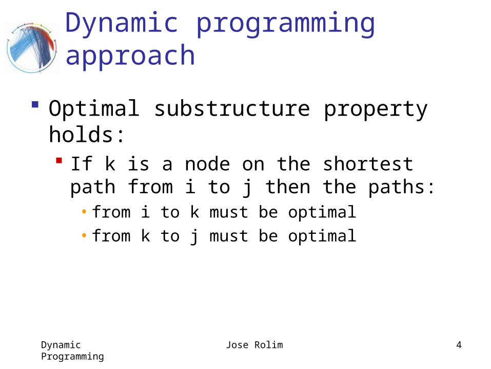
Optimal substructure property holds: If k is a node on the shortest path from i
to j then the paths:• from i to k must be optimal• from k to j must be optimal
Dynamic Programming Jose Rolim 5
Recursive solution
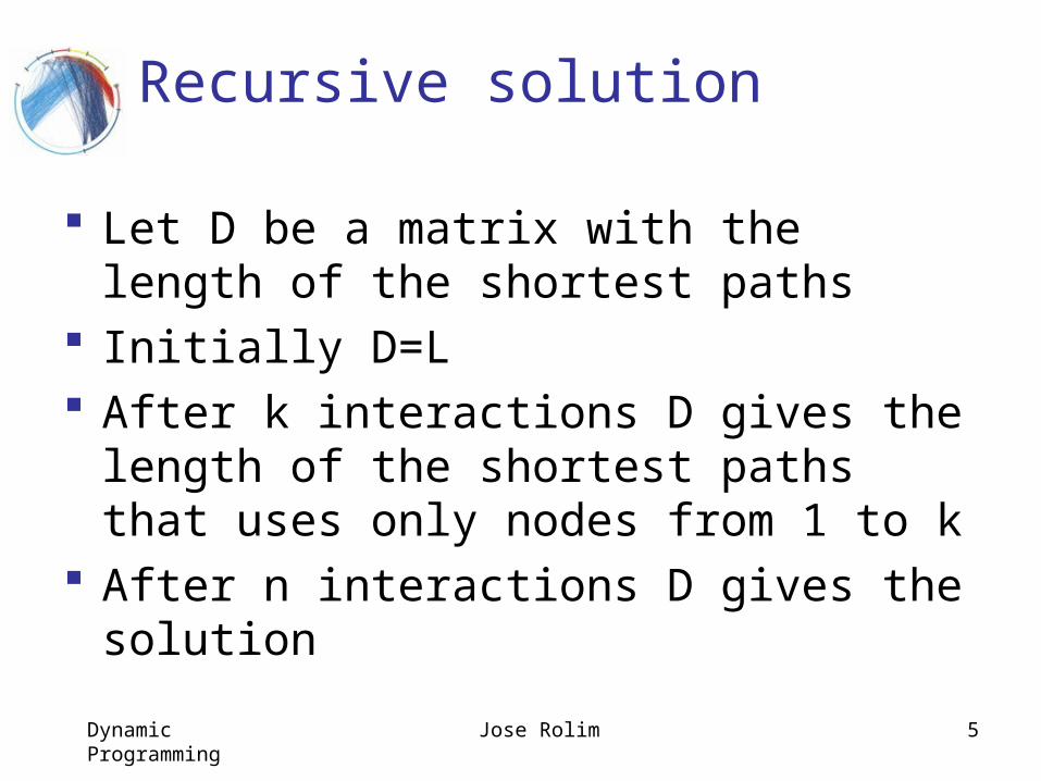
Let D be a matrix with the length of the shortest paths
Initially D=L After k interactions D gives the
length of the shortest paths that uses only nodes from 1 to k
After n interactions D gives the solution
Dynamic Programming Jose Rolim 6
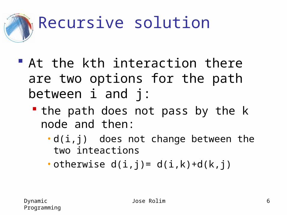
Recursive solution
At the kth interaction there are two options for the path between i and j: the path does not pass by the k node
and then:• d(i,j) does not change between the two
inteactions• otherwise d(i,j)= d(i,k)+d(k,j)
Dynamic Programming Jose Rolim 7
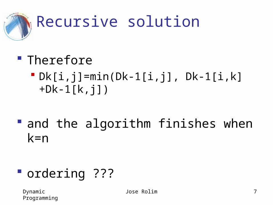
Recursive solution
Therefore Dk[i,j]=min(Dk-1[i,j], Dk-1[i,k]+Dk-
1[k,j])
and the algorithm finishes when k=n
ordering ???
Dynamic Programming Jose Rolim 8
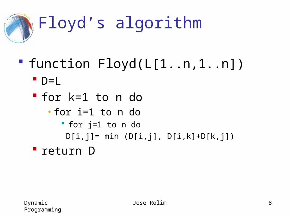
Floyd’s algorithm
function Floyd(L[1..n,1..n]) D=L for k=1 to n do
• for i=1 to n do for j=1 to n do D[i,j]= min (D[i,j], D[i,k]+D[k,j])
return D
Dynamic Programming Jose Rolim 9
Remarks
Complexity O(n**3)
To get the paths we can use a second matrix for the nodes k used in the path
Negative lenghts?
Longest paths?
Dynamic Programming Jose Rolim 10
Review: Dynamic programming
DP is a method for solving certain kind of problems
DP can be applied when the solution of a problem includes solutions to subproblems
We need to find a recursive formula for the solution
We can recursively solve subproblems, starting from the trivial case, and save their solutions in memory in a convenient order
In the end we’ll get the solution of the whole problem

Dynamic Programming Jose Rolim 11
Properties of a problem that can be solved with dynamic programming Simple Subproblems
We should be able to break the original problem to smaller subproblems that have the same structure
Optimal Substructure of the problems The solution to the problem must be a
composition of subproblem solutions Subproblem Overlap
Optimal subproblems to unrelated problems can contain subproblems in common

Dynamic Programming Jose Rolim 12
0-1 Knapsack problem
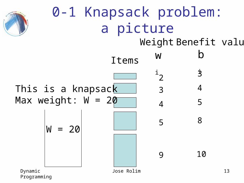
Given a knapsack with maximum capacity W, and a set S consisting of n items
Each item i has some weight wi and benefit
value bi (all wi , bi and W are integer values)
Problem: How to pack the knapsack to achieve maximum total value of packed items?
Dynamic Programming Jose Rolim 13
0-1 Knapsack problem:a picture
W = 20
wi bi
109
85
54
43
32
Weight Benefit value
This is a knapsackMax weight: W = 20
Items
Dynamic Programming Jose Rolim 14
0-1 Knapsack problem
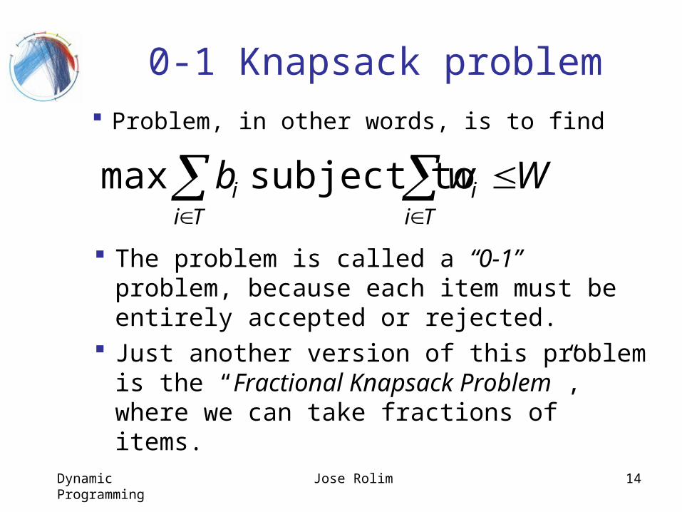
Problem, in other words, is to find
Ti
iTi
i Wwb subject to max
The problem is called a “0-1” problem, because each item must be entirely accepted or rejected.
Just another version of this problem is the “Fractional Knapsack Problem”, where we can take fractions of items.
Dynamic Programming Jose Rolim 15
Brute-force approach
Let’s first solve this problem with a straightforward algorithm
Since there are n items, there are 2n possible combinations of items.
We go through all combinations and find the one with the most total value and with total weight less or equal to W
Running time will be O(2n)
Dynamic Programming Jose Rolim 16
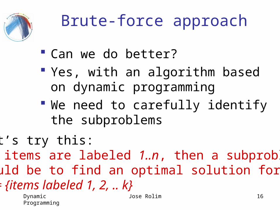
Brute-force approach
Can we do better? Yes, with an algorithm based on dynamic
programming We need to carefully identify the
subproblems
Let’s try this:If items are labeled 1..n, then a subproblem would be to find an optimal solution for Sk = {items labeled 1, 2, .. k}
Dynamic Programming Jose Rolim 17
Defining a Subproblem
This is a valid subproblem definition.
The question is: can we describe the final solution (Sn ) in terms of subproblems (Sk)?
Unfortunately, we can’t do that.
Dynamic Programming Jose Rolim 18
Defining a Subproblem
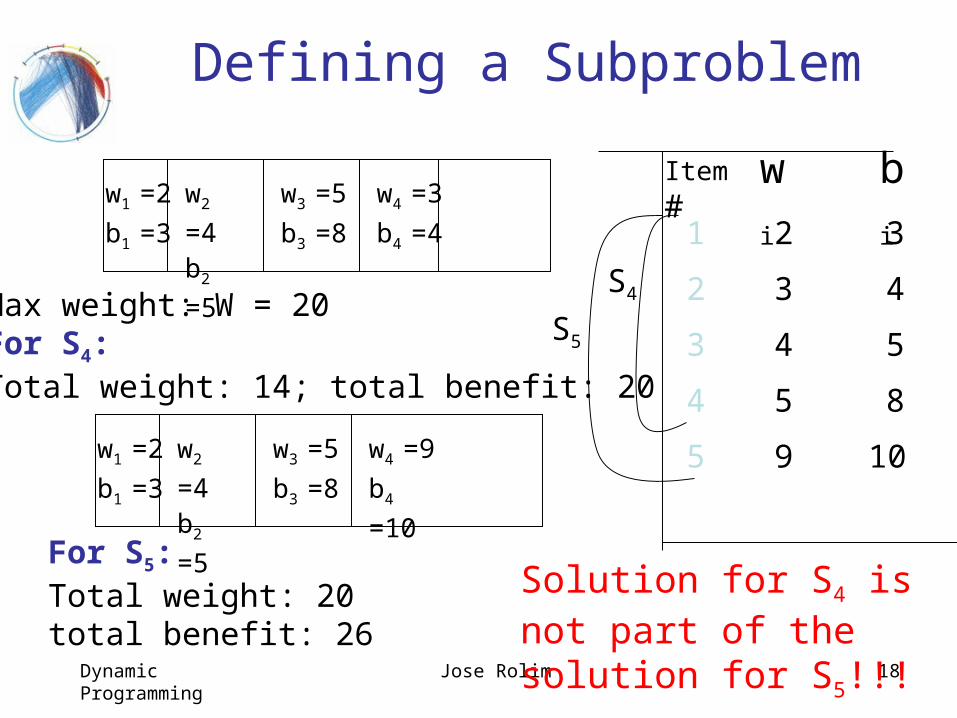
Max weight: W = 20For S4:Total weight: 14; total benefit: 20
w1 =2
b1 =3
w2 =4
b2 =5
w3 =5
b3 =8
w4 =3
b4 =4
wi bi
10
85
54
43
32
9
Item
#
4
3
2
1
5
S4
S5
w1 =2
b1 =3
w2 =4
b2 =5
w3 =5
b3 =8
w4 =9
b4 =10
For S5:Total weight: 20total benefit: 26
Solution for S4 is not part of the solution for S5!!!
Dynamic Programming Jose Rolim 19
Defining a Subproblem
As we have seen, the solution for S4 is not part of the solution for S5
So our definition of a subproblem is flawed and we need another one!
Let’s add another parameter: w, which will represent the exact weight for each subset of items
The subproblem then will be to compute B[k,w]
Dynamic Programming Jose Rolim 20
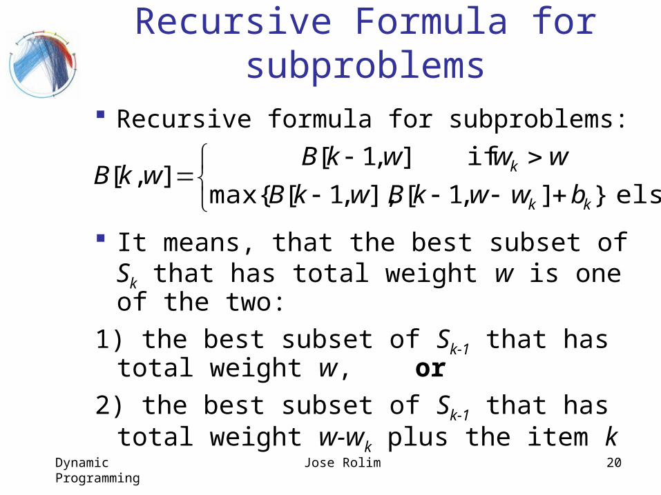
Recursive Formula for subproblems
It means, that the best subset of Sk that has total weight w is one of the two:
1) the best subset of Sk-1 that has total weight w, or
2) the best subset of Sk-1 that has total weight w-wk plus the item k
else }],1[],,1[max{
if ],1[],[
kk
k
bwwkBwkB
wwwkBwkB
Recursive formula for subproblems:
Dynamic Programming Jose Rolim 21
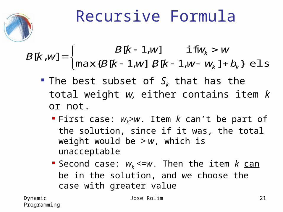
Recursive Formula
The best subset of Sk that has the total weight w, either contains item k or not. First case: wk>w. Item k can’t be part of the
solution, since if it was, the total weight would be > w, which is unacceptable
Second case: wk <=w. Then the item k can be in the solution, and we choose the case with greater value
else }],1[],,1[max{
if ],1[],[
kk
k
bwwkBwkB
wwwkBwkB
Dynamic Programming Jose Rolim 22
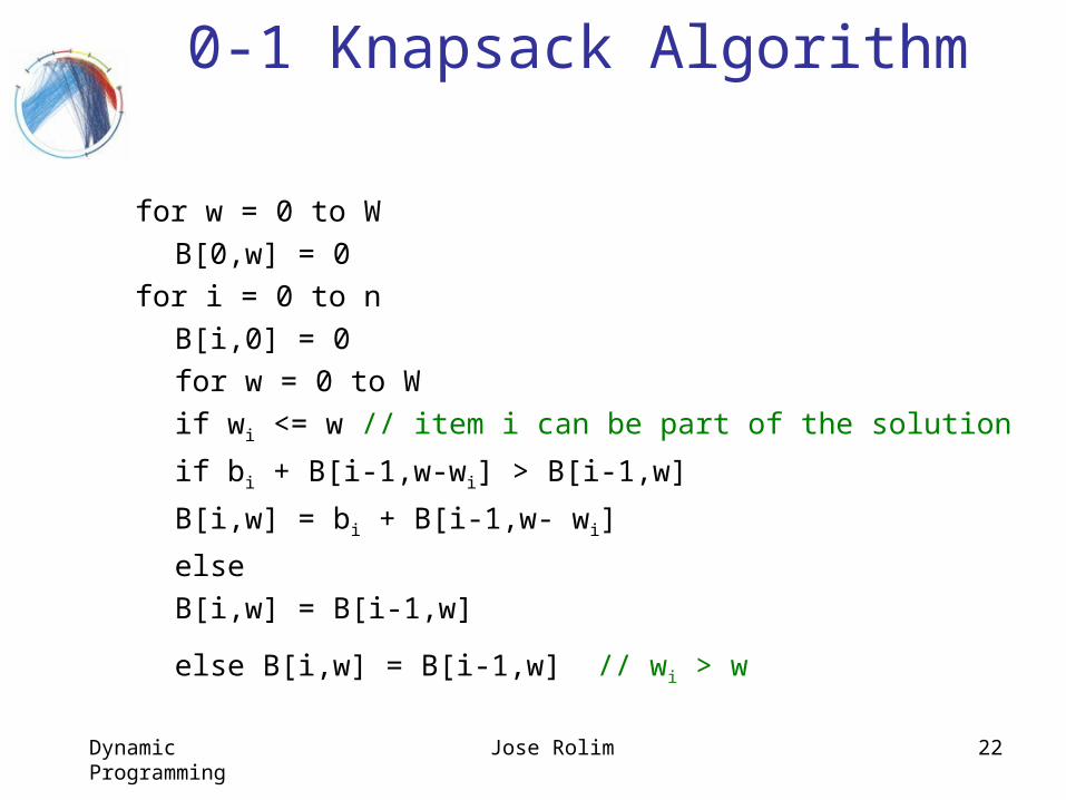
0-1 Knapsack Algorithm
for w = 0 to W
B[0,w] = 0
for i = 0 to n
B[i,0] = 0
for w = 0 to W
if wi <= w // item i can be part of the solution
if bi + B[i-1,w-wi] > B[i-1,w]
B[i,w] = bi + B[i-1,w- wi]
else
B[i,w] = B[i-1,w]
else B[i,w] = B[i-1,w] // wi > w
Dynamic Programming Jose Rolim 23
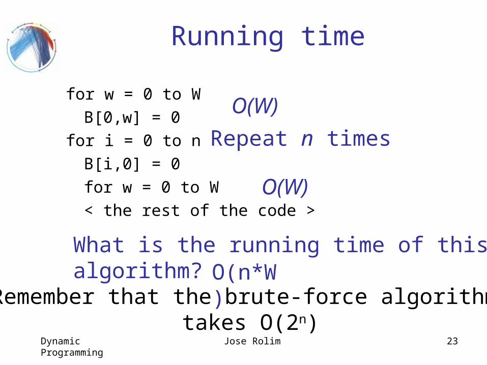
Running time
for w = 0 to W
B[0,w] = 0
for i = 0 to n
B[i,0] = 0
for w = 0 to W
< the rest of the code >
What is the running time of this algorithm?
O(W)
O(W)
Repeat n times
O(n*W)Remember that the brute-force algorithm
takes O(2n)
Dynamic Programming Jose Rolim 24
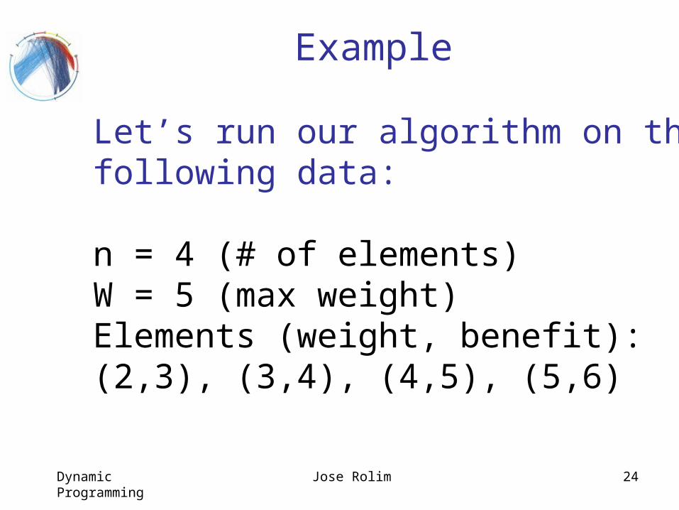
Example
Let’s run our algorithm on the following data:
n = 4 (# of elements)W = 5 (max weight)Elements (weight, benefit):(2,3), (3,4), (4,5), (5,6)
Dynamic Programming Jose Rolim 25
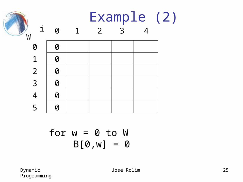
Example (2)
for w = 0 to WB[0,w] = 0
0
0
0
0
0
0
W0
1
2
3
4
5
i 0 1 2 3
4
Dynamic Programming Jose Rolim 26
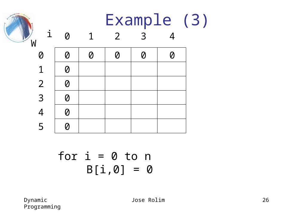
Example (3)
for i = 0 to nB[i,0] = 0
0
0
0
0
0
0
W0
1
2
3
4
5
i 0 1 2 3
0 0 0 0
4
Dynamic Programming Jose Rolim 27
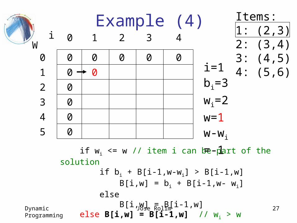
Example (4)
if wi <= w // item i can be part of the solution if bi + B[i-1,w-wi] > B[i-1,w] B[i,w] = bi + B[i-1,w- wi] else B[i,w] = B[i-1,w] else B[i,w] = B[i-1,w] // wi > w
0
0
0
0
0
0
W0
1
2
3
4
5
i 0 1 2 3
0 0 0 0i=1bi=3
wi=2
w=1w-wi =-1
Items:1: (2,3)2: (3,4)3: (4,5) 4: (5,6)
4
0
Dynamic Programming Jose Rolim 28
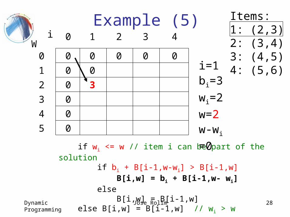
Example (5)
if wi <= w // item i can be part of the solution if bi + B[i-1,w-wi] > B[i-1,w] B[i,w] = bi + B[i-1,w- wi] else B[i,w] = B[i-1,w] else B[i,w] = B[i-1,w] // wi > w
0
0
0
0
0
0
W0
1
2
3
4
5
i 0 1 2 3
0 0 0 0i=1bi=3
wi=2
w=2w-wi =0
Items:1: (2,3)2: (3,4)3: (4,5) 4: (5,6)
4
0
3
Dynamic Programming Jose Rolim 29
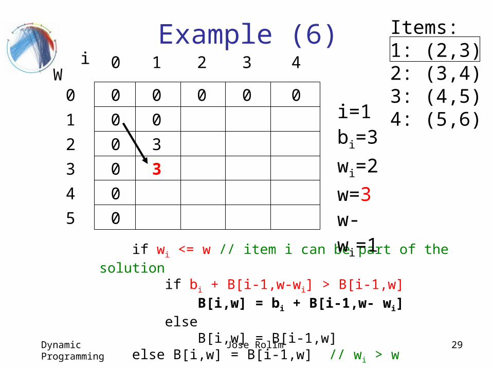
Example (6)
if wi <= w // item i can be part of the solution if bi + B[i-1,w-wi] > B[i-1,w] B[i,w] = bi + B[i-1,w- wi] else B[i,w] = B[i-1,w] else B[i,w] = B[i-1,w] // wi > w
0
0
0
0
0
0
W0
1
2
3
4
5
i 0 1 2 3
0 0 0 0i=1bi=3
wi=2
w=3w-wi=1
Items:1: (2,3)2: (3,4)3: (4,5) 4: (5,6)
4
0
3
3
Dynamic Programming Jose Rolim 30
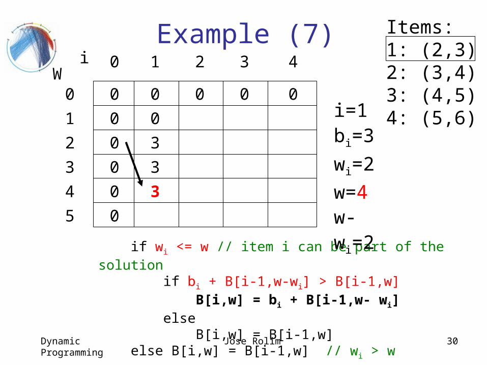
Example (7)
if wi <= w // item i can be part of the solution if bi + B[i-1,w-wi] > B[i-1,w] B[i,w] = bi + B[i-1,w- wi] else B[i,w] = B[i-1,w] else B[i,w] = B[i-1,w] // wi > w
0
0
0
0
0
0
W0
1
2
3
4
5
i 0 1 2 3
0 0 0 0i=1bi=3
wi=2
w=4w-wi=2
Items:1: (2,3)2: (3,4)3: (4,5) 4: (5,6)
4
0
3
3
3
Dynamic Programming Jose Rolim 31
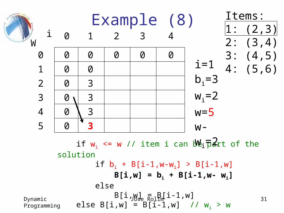
Example (8)
if wi <= w // item i can be part of the solution if bi + B[i-1,w-wi] > B[i-1,w] B[i,w] = bi + B[i-1,w- wi] else B[i,w] = B[i-1,w] else B[i,w] = B[i-1,w] // wi > w
0
0
0
0
0
0
W0
1
2
3
4
5
i 0 1 2 3
0 0 0 0i=1bi=3
wi=2
w=5w-wi=2
Items:1: (2,3)2: (3,4)3: (4,5) 4: (5,6)
4
0
3
3
3
3
Dynamic Programming Jose Rolim 32
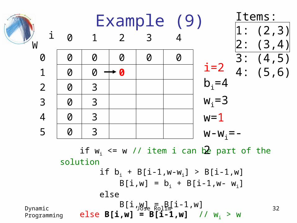
Example (9)
if wi <= w // item i can be part of the solution if bi + B[i-1,w-wi] > B[i-1,w] B[i,w] = bi + B[i-1,w- wi] else B[i,w] = B[i-1,w] else B[i,w] = B[i-1,w] // wi > w
0
0
0
0
0
0
W0
1
2
3
4
5
i 0 1 2 3
0 0 0 0i=2bi=4
wi=3
w=1w-wi=-2
Items:1: (2,3)2: (3,4)3: (4,5) 4: (5,6)
4
0
3
3
3
3
0
Dynamic Programming Jose Rolim 33
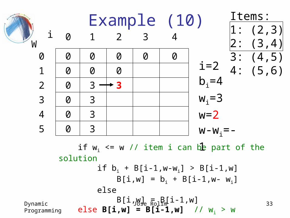
Example (10)
if wi <= w // item i can be part of the solution if bi + B[i-1,w-wi] > B[i-1,w] B[i,w] = bi + B[i-1,w- wi] else B[i,w] = B[i-1,w] else B[i,w] = B[i-1,w] // wi > w
0
0
0
0
0
0
W0
1
2
3
4
5
i 0 1 2 3
0 0 0 0i=2bi=4
wi=3
w=2w-wi=-1
Items:1: (2,3)2: (3,4)3: (4,5) 4: (5,6)
4
0
3
3
3
3
0
3
Dynamic Programming Jose Rolim 34
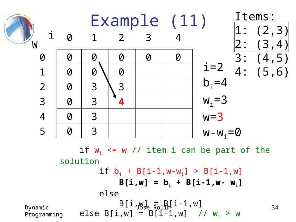
Example (11)
if wi <= w // item i can be part of the solution if bi + B[i-1,w-wi] > B[i-1,w] B[i,w] = bi + B[i-1,w- wi] else B[i,w] = B[i-1,w] else B[i,w] = B[i-1,w] // wi > w
0
0
0
0
0
0
W0
1
2
3
4
5
i 0 1 2 3
0 0 0 0i=2bi=4
wi=3
w=3w-wi=0
Items:1: (2,3)2: (3,4)3: (4,5) 4: (5,6)
4
0
3
3
3
3
0
3
4
Dynamic Programming Jose Rolim 35
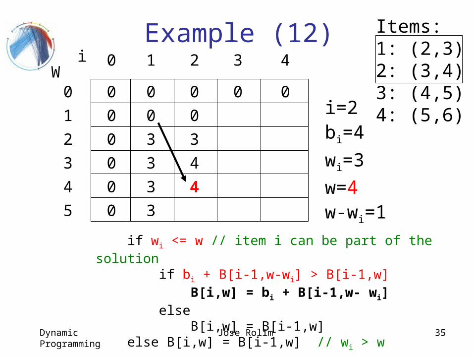
Example (12)
if wi <= w // item i can be part of the solution if bi + B[i-1,w-wi] > B[i-1,w] B[i,w] = bi + B[i-1,w- wi] else B[i,w] = B[i-1,w] else B[i,w] = B[i-1,w] // wi > w
0
0
0
0
0
0
W0
1
2
3
4
5
i 0 1 2 3
0 0 0 0i=2bi=4
wi=3
w=4w-wi=1
Items:1: (2,3)2: (3,4)3: (4,5) 4: (5,6)
4
0
3
3
3
3
0
3
4
4
Dynamic Programming Jose Rolim 36
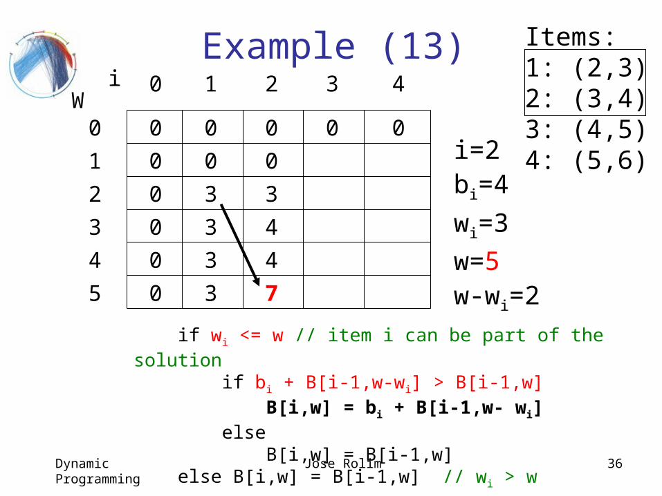
Example (13)
if wi <= w // item i can be part of the solution if bi + B[i-1,w-wi] > B[i-1,w] B[i,w] = bi + B[i-1,w- wi] else B[i,w] = B[i-1,w] else B[i,w] = B[i-1,w] // wi > w
0
0
0
0
0
0
W0
1
2
3
4
5
i 0 1 2 3
0 0 0 0i=2bi=4
wi=3
w=5w-wi=2
Items:1: (2,3)2: (3,4)3: (4,5) 4: (5,6)
4
0
3
3
3
3
0
3
4
4
7
Dynamic Programming Jose Rolim 37
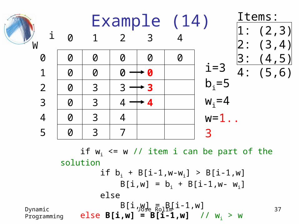
Example (14)
if wi <= w // item i can be part of the solution if bi + B[i-1,w-wi] > B[i-1,w] B[i,w] = bi + B[i-1,w- wi] else B[i,w] = B[i-1,w] else B[i,w] = B[i-1,w] // wi > w
0
0
0
0
0
0
W0
1
2
3
4
5
i 0 1 2 3
0 0 0 0i=3bi=5
wi=4
w=1..3
Items:1: (2,3)2: (3,4)3: (4,5) 4: (5,6)
4
0
3
3
3
3
00
3
4
4
7
0
3
4
Dynamic Programming Jose Rolim 38
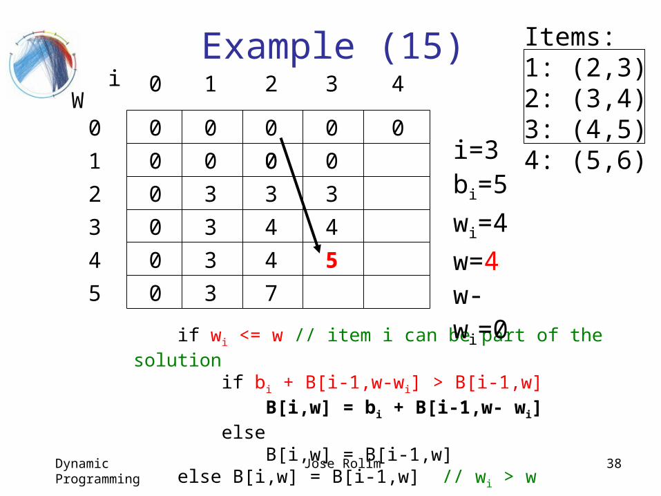
Example (15)
if wi <= w // item i can be part of the solution if bi + B[i-1,w-wi] > B[i-1,w] B[i,w] = bi + B[i-1,w- wi] else B[i,w] = B[i-1,w] else B[i,w] = B[i-1,w] // wi > w
0
0
0
0
0
0
W0
1
2
3
4
5
i 0 1 2 3
0 0 0 0i=3bi=5
wi=4
w=4w- wi=0
Items:1: (2,3)2: (3,4)3: (4,5) 4: (5,6)
4
0 00
3
4
4
7
0
3
4
5
3
3
3
3
Dynamic Programming Jose Rolim 39
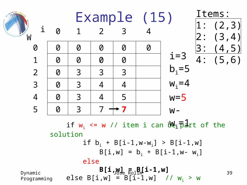
Example (15)
if wi <= w // item i can be part of the solution if bi + B[i-1,w-wi] > B[i-1,w] B[i,w] = bi + B[i-1,w- wi] else B[i,w] = B[i-1,w] else B[i,w] = B[i-1,w] // wi > w
0
0
0
0
0
0
W0
1
2
3
4
5
i 0 1 2 3
0 0 0 0i=3bi=5
wi=4
w=5w- wi=1
Items:1: (2,3)2: (3,4)3: (4,5) 4: (5,6)
4
0 00
3
4
4
7
0
3
4
5
7
3
3
3
3
Dynamic Programming Jose Rolim 40
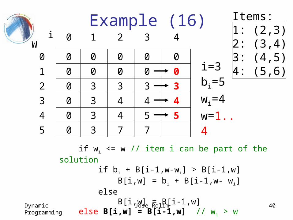
Example (16)
if wi <= w // item i can be part of the solution if bi + B[i-1,w-wi] > B[i-1,w] B[i,w] = bi + B[i-1,w- wi] else B[i,w] = B[i-1,w] else B[i,w] = B[i-1,w] // wi > w
0
0
0
0
0
0
W0
1
2
3
4
5
i 0 1 2 3
0 0 0 0i=3bi=5
wi=4
w=1..4
Items:1: (2,3)2: (3,4)3: (4,5) 4: (5,6)
4
0 00
3
4
4
7
0
3
4
5
7
0
3
4
5
3
3
3
3
Dynamic Programming Jose Rolim 41
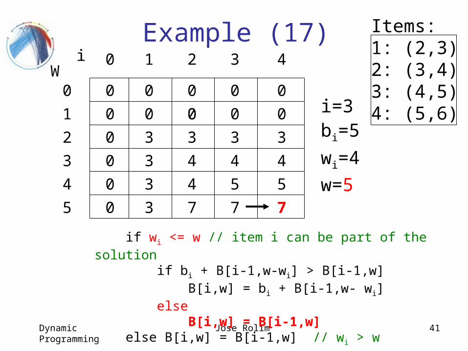
Example (17)
if wi <= w // item i can be part of the solution if bi + B[i-1,w-wi] > B[i-1,w] B[i,w] = bi + B[i-1,w- wi] else B[i,w] = B[i-1,w] else B[i,w] = B[i-1,w] // wi > w
0
0
0
0
0
0
W0
1
2
3
4
5
i 0 1 2 3
0 0 0 0i=3bi=5
wi=4
w=5
Items:1: (2,3)2: (3,4)3: (4,5) 4: (5,6)
4
0 00
3
4
4
7
0
3
4
5
7
0
3
4
5
7
3
3
3
3
Dynamic Programming Jose Rolim 42
Comments
This algorithm only finds the max possible value that can be carried in the knapsack
To know the items that make this maximum value, an addition to this algorithm is necessary
Dynamic Programming Jose Rolim 43
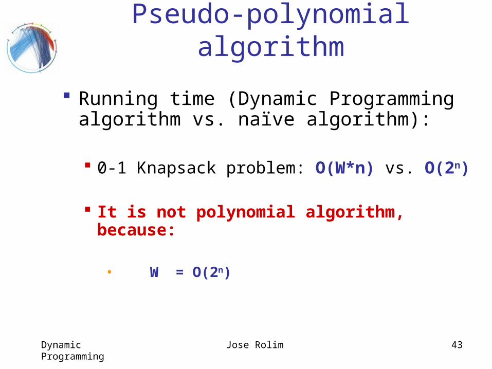
Pseudo-polynomial algorithm
Running time (Dynamic Programming algorithm vs. naïve algorithm):
0-1 Knapsack problem: O(W*n) vs. O(2n)
It is not polynomial algorithm, because:
• W = O(2n)
Dynamic Programming Jose Rolim 44
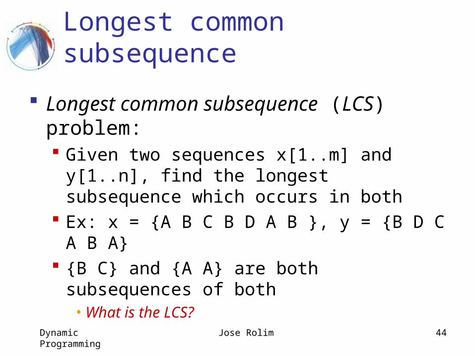
Longest common subsequence
Longest common subsequence (LCS) problem: Given two sequences x[1..m] and y[1..n],
find the longest subsequence which occurs in both
Ex: x = {A B C B D A B }, y = {B D C A B A}
{B C} and {A A} are both subsequences of both• What is the LCS?
Dynamic Programming Jose Rolim 45
Brute force algorithm
Brute-force algorithm:
For every subsequence of x, check if it’s a subsequence of y• How many subsequences of x are there?• What will be the running time of the brute-
force algorithm?
Dynamic Programming Jose Rolim 46
Running time: brute force algorithm
Brute-force algorithm: 2m subsequences of x to check
against n elements of y: O(n 2m)
Dynamic Programming Jose Rolim 47
LCS Algorithm
Let’s only worry about the problem of finding the length of LCS
Define c[i,j] to be the length of the LCS of x[1..i] and y[1..j]
Initial cases: c[0,j] = c[i,0] = 0
Dynamic Programming Jose Rolim 48
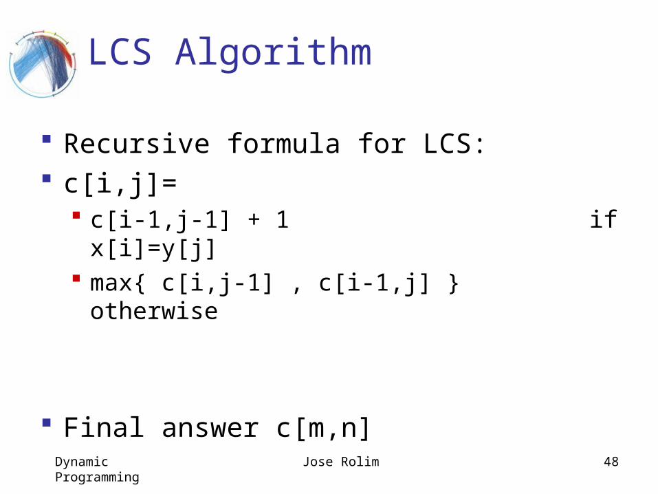
LCS Algorithm
Recursive formula for LCS: c[i,j]=
c[i-1,j-1] + 1 if x[i]=y[j] max{ c[i,j-1] , c[i-1,j] } otherwise
Final answer c[m,n]
Dynamic Programming Jose Rolim 49
Running time
After we have filled the array c[ ], we can backtrack to find the characters that constitute the Longest Common Subsequence
Algorithm runs in O(m*n), which is much better than the brute-force algorithm: O(n 2m)
Dynamic Programming Jose Rolim 50
Conclusions
Dynamic Programming is an algorithm design method that can be used when the solution to a problem may be viewed as the result of a sequence of decisions (Ordering) and:
Dynamic Programming Jose Rolim 51
Conclusions
Principle of optimality: Suppose that in solving a problem, we have to make a sequence of decisions D1, D2, …, Dn. If this sequence is optimal, then the last k decisions, 1 k n must be optimal.
In summary, if a problem can be described by this principle, then it can be solved by dynamic programming.