Embed Size (px)
Citation preview

3
Topics
What it is
How it works: Resonance
Error estimates
Detailed example: Lifetime
Several Parameters
Extended maximum L
Do’s and Dont’s with L

4
• NORMALISATION FOR LIKELIHOOD
• JUST QUOTE UPPER LIMIT
• (ln L) = 0.5 RULE
• Lmax AND GOODNESS OF FIT
•
• BAYESIAN SMEARING OF L
• USE CORRECT L (PUNZI EFFECT)
90.0 dp ppU
L
L
DO’S AND DONT’S WITH L

5

6
How it works: Resonance
y ~ Γ/2
(m-M0)2 + (Γ/2)2
m m
Vary M0
Vary Γ

7

8

9
Maximum L errorLikely values of μ from width of L(μ) distributionIf L(μ) is Gaussian, following definitions of σ are equivalent:1) RMS of L(µ)
2) 1/√(-d2lnL/dµ2) 3) ln(L(μ±σ)) = ln(L(μ0)) -1/2If L(μ) is non-Gaussian, these are no longer the same
“Procedure 3) above still gives interval that contains the true value of parameter μ with 68% probability”
Asymmetric errors (e.g. from method 3)) are messy, so try to choose variables sensibly e.g. 1/p rather than p
τ or λ

10

11

12

13

14

15

16
• NORMALISATION FOR LIKELIHOOD
• JUST QUOTE UPPER LIMIT
• (ln L) = 0.5 RULE
• Lmax AND GOODNESS OF FIT
•
• BAYESIAN SMEARING OF L
• USE CORRECT L (PUNZI EFFECT)
90.0 dp ppU
L
L
DO’S AND DONT’S WITH L

17
NORMALISATION FOR LIKELIHOOD
dx )|P(x
data param
e.g. Lifetime fit to t1, t2,………..tn
t
big too
Reasonable
MUST be independent of
/1 Missing
/ )|(
tetPINCORRECT

18
2) QUOTING UPPER LIMIT
“We observed no significant signal, and our 90% conf upper limit is …..”
Need to specify method e.g.
L
Chi-squared (data or theory error)
Frequentist (Central or upper limit)
Feldman-Cousins
Bayes with prior = const,
“Show your L” ***
1) Not always practical
2) Not sufficient for frequentist methods
etc 1/ /1

19
90% C.L. Upper Limits
x
x0

20
ΔlnL = -1/2 ruleIf L(μ) is Gaussian, following definitions of σ are
equivalent:
1) RMS of L(µ)
2) 1/√(-d2lnL/dµ2) 3) ln(L(μ±σ) = ln(L(μ0)) -1/2
If L(μ) is non-Gaussian, these are no longer the same
“Procedure 3) above still gives interval that contains the true value of parameter μ with 68% probability”
Heinrich: CDF note 6438 (see CDF Statistics Committee Web-page)
Barlow: Phystat05

21
COVERAGE
How often does quoted range for parameter include param’s true value?
N.B. Coverage is a property of METHOD, not of a particular exptl result
Coverage can vary with μ
Study coverage of different methods of Poisson parameter μ, from observation of number of events n
Hope for: Nominal value
100%
)(C

22
COVERAGE
If true for all μ: “Correct coverage”
P< α for some μ “Undercoverage” (this is serious !)
P> α for some μ “Overcoverage”
Conservative
Loss of rejection power

23
Coverage : L approach (Not frequentist)
P(n,μ) = e-μμn/n! (Joel Heinrich CDF note 6438)
-2 lnλ< 1 λ = P(n,μ)/P(n,μbest) UNDERCOVERS

24
Frequentist central intervals, NEVER undercovers
(Conservative at both ends)

25
Feldman-Cousins Unified intervals
Frequentist, so NEVER undercovers

26
Probability ordering
Frequentist, so NEVER undercovers

27
= (n-µ)2/µ Δ = 0.1 24.8% coverage?
NOT frequentist : Coverage = 0% 100%
22

28
Great?Good?Bad
Lmax
Frequency
Unbinned Lmax and Goodness of Fit?
Find params by maximising L
So larger L better than smaller L
So Lmax gives Goodness of Fit ??
Monte Carlo distribution
of unbinned Lmax

29
Not necessarily: pdf L(data,params) fixed vary L Contrast pdf(data,params) param
vary fixed data
e.g. p(λ) = λ exp(-λt) Max at t = 0 Max at λ = 1/t p L
t λ
30
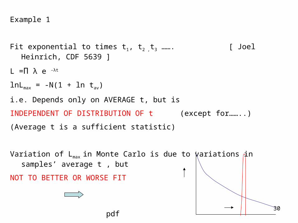
Example 1
Fit exponential to times t1, t2 ,t3 ……. [ Joel Heinrich, CDF 5639 ]
L =Π λ e -λt
lnLmax = -N(1 + ln tav)
i.e. Depends only on AVERAGE t, but is
INDEPENDENT OF DISTRIBUTION OF t (except for……..)
(Average t is a sufficient statistic)
Variation of Lmax in Monte Carlo is due to variations in samples’ average t , but
NOT TO BETTER OR WORSE FIT
Same average t same Lmax
t

31
Example 2
L =
cos θ
pdf (and likelihood) depends only on cos2θi
Insensitive to sign of cosθi
So data can be in very bad agreement with expected distribution
e.g. all data with cosθ < 0
and Lmax does not know about it.
Example of general principle
3/1cos1
cos
2
d
dN
i3/1
cos1 i2

32
Example 3
Fit to Gaussian with variable μ, fixed σ
lnLmax = N(-0.5 ln2π – lnσ) – 0.5 Σ(xi – xav)2 /σ2
constant ~variance(x)
i.e. Lmax depends only on variance(x),
which is not relevant for fitting μ (μest = xav)
Smaller than expected variance(x) results in larger Lmax
x
x
Worse fit, larger Lmax Better fit, lower Lmax
}{2
2
1exp
2
1
x

33
Lmax and Goodness of Fit?
Conclusion:
L has sensible properties with respect to parameters
NOT with respect to data
Lmax within Monte Carlo peak is NECESSARY
not SUFFICIENT
(‘Necessary’ doesn’t mean that you have to do it!)

34
Binned data and Goodness of Fit using L-ratio
i
iP ni )(ni L =
μi Lbest
x
ln[L-ratio] = ln[L/Lbest]
large μi -0.52 i.e. Goodness of Fit
μbest is independent of parameters of fit,
and so same parameter values from L or L-ratio
Baker and Cousins, NIM A221 (1984) 437
)(
),(
i
i
n
i
nP
bestiP ni
i

35
L and pdf
Example 1: Poissonpdf = Probability density function for observing n, given μ P(n;μ) = e -μ μn/n!From this, construct L as L(μ;n) = e -μ μn/n!i.e. use same function of μ and n, but . . . . . . . . . .
pdf for pdf, μ is fixed, but for L, n is fixed μ L
n
N.B. P(n;μ) exists only at integer non-negative n L(μ;n) exists only as continuous function of non-negative μ

36
xample 2 Lifetime distribution
pdf p(t;λ) = λ e -λt
So L(λ;t) = λ e –λt (single observed t)
Here both t and λ are continuous
pdf maximises at t = 0
L maximises at λ = t
. Functionalform of P(t) and L(λ) are different
Fixed λ Fixed t
p L
t λ

37
Example 3: Gaussian
N.B. In this case, same functional form for pdf and L
So if you consider just Gaussians, can be confused between pdf and L
So examples 1 and 2 are useful
}{ 2
2
2
)(exp
2
1);(
x
xpdf
}{ 2
2
2
)(exp
2
1);(
x
xL

38
Transformation properties of pdf and L
Lifetime example: dn/dt = λ e –λt
Change observable from t to y = √t
So (a) pdf changes, BUT (b)
i.e. corresponding integrals of pdf are INVARIANT
22 yey
dydt
dtdn
dydn
dydydn
dtdtdn
tt
00

39
Now for Likelihood
When parameter changes from λ to τ = 1/λ
(a’) L does not change
dn/dt = 1/τ exp{-t/τ}
and so L(τ;t) = L(λ=1/τ;t)
because identical numbers occur in evaluations of the two L’s
BUT
(b’)
So it is NOT meaningful to integrate L
(However,………)
0
0
);();(0
dtLdtL
40
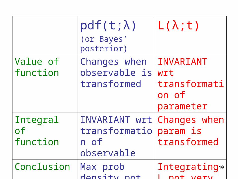
pdf(t;λ)(or Bayes’ posterior)
L(λ;t)
Value of function
Changes when observable is transformed
INVARIANT wrt transformation of parameter
Integral of function
INVARIANT wrt transformation of observable
Changes when param is transformed
Conclusion Max prob density not very sensible
Integrating L not very sensible

41
CONCLUSION:
NOT recognised statistical procedure
[Metric dependent:
τ range agrees with τpred
λ range inconsistent with 1/τpred ]
BUT
1) Could regard as “black box”
2) Make respectable by L Bayes’ posterior , via Bayes’ prior
Posterior(λ) ~ L(λ)* Prior(λ) [and Prior(λ) can be constant]
u
l
p
p
dpL

42

43
Getting L wrong: Punzi effect
Giovanni Punzi @ PHYSTAT2003“Comments on L fits with variable resolution”
Separate two close signals, when resolution σ varies event by event, and is different for 2 signals
e.g. 1) Signal 1 1+cos2θ Signal 2 Isotropic and different parts of detector give different σ
2) M (or τ) Different numbers of tracks different σM (or στ)

44
Events characterised by xi andσi
A events centred on x = 0
B events centred on x = 1
L(f)wrong = Π [f * G(xi,0,σi) + (1-f) * G(xi,1,σi)]
L(f)right = Π [f*p(xi,σi;A) + (1-f) * p(xi,σi;B)]
p(S,T) = p(S|T) * p(T)
p(xi,σi|A) = p(xi|σi,A) * p(σi|A)
= G(xi,0,σi) * p(σi|A)
So
L(f)right = Π[f * G(xi,0,σi) * p(σi|A) + (1-f) * G(xi,1,σi) * p(σi|B)]
If p(σ|A) = p(σ|B), Lright = Lwrong
but NOT otherwise

45
Giovanni’s Monte Carlo for A : G(x,0, )
B : G(x,1)
fA = 1/3
Lwrong Lright
fAffAf
1.0 1.0 0.336(3) 0.08 Same
1.0 1.1 0.374(4) 0.08 0. 333(0) 0
1.0 2.00.645(6) 0.12 0.333(0)0
1 2 1.5 3 0.514(7) 0.14 0.335(2) 0.03
1.0 1 2 0.482(9) 0.09 0.333(0) 0
1) Lwrong OK for pp, but otherwise BIASSED
2) Lright unbiassed, but Lwrong biassed (enormously)!
3) Lright gives smaller σf than Lwrong

46
Explanation of Punzi bias
σA = 1 σB = 2
A events with σ = 1
B events with σ = 2
x x
ACTUAL DISTRIBUTION FITTING FUNCTION
[NA/NB variable, but same for A and B events]
Fit gives upward bias for NA/NB because (i) that is much better for A events; and
(ii) it does not hurt too much for B events

47
Another scenario for Punzi problem: PID A B π K
M TOF
Originally:
Positions of peaks = constant K-peak π-peak at large momentum
σi variable, (σi)A = (σi)B σi ~ constant, pK = pπ
COMMON FEATURE: Separation/Error = Constant
Where else??
MORAL: Beware of event-by-event variables whose pdf’s do not
appear in L

48
Avoiding Punzi Bias
• Include p(σ|A) and p(σ|B) in fit (But then, for example, particle identification may be determined
more by momentum distribution than by PID) OR• Fit each range of σi separately, and add (NA)i (NA)total, and similarly for B
Incorrect method using Lwrong uses weighted average of (fA)j, assumed to be independent of j
Talk by Catastini at PHYSTAT05

50
CONCLUSIONS
“Maximum Likelihood” is a powerful method of parameter determination
Error estimates typically do not have good coverage properties
For unbinned likelihoods, the value of Lmax usually does not provide a measure of “Goodness of Fit”
Writing the likelihood correctly requires care
Be especially careful with event-dependent variables

51
TOMORROW
11am N.B. ******
“Discovery issues”
4pm “Bayes and Frequentism: the return of an old controvery”