28th International North Sea Flow Measurement Workshop

26th – 29

th October 2010

1

Developments in the Self-Diagnostic Capabilities of Orifice Plate Meters

Mark Skelton, BP Exploration Operating Company Ltd.

Simon Barrons, ConocoPhillips UK Ltd.

Jennifer Ayre, Swinton Technology Ltd.

Richard Steven, DP Diagnostics Llc.

1. Introduction

In 2008 [1] & 2009 [2] DP Diagnostics disclosed a generic differential pressure (DP) meter diagnostic

methodology. Swinton Technology (ST) has subsequently developed the solution “Prognosis” in

partnership with DP Diagnostics. Prognosis allows these generic DP meter diagnostic methodologies to

be applied via software on a PC automatically reading live instrument signals thereby making these

principles available for field applications.

Whereas initial DP Diagnostics technical papers concentrated on proving the diagnostic principles a

simple way of presenting the diagnostic results was also proposed. The diagnostic analysis could be

plotted as points on a graph which could be shown live in a control room (or archived for later

analysis). After a review of the diagnostic methods this paper discusses diagnostic pattern recognition

for this graphical representation. It can be shown that when the diagnostics signal a warning the pattern

of points can indicate extra information regarding the source of the problem. New CEESI Iowa test

facility, BP Central Area Transmission System and ConocoPhillips Theddlethorpe gas terminal large

orifice meter data sets are presented here showing these principles.

2. A Review of the Fundamental Diagnostics for Orifice Plate Meters

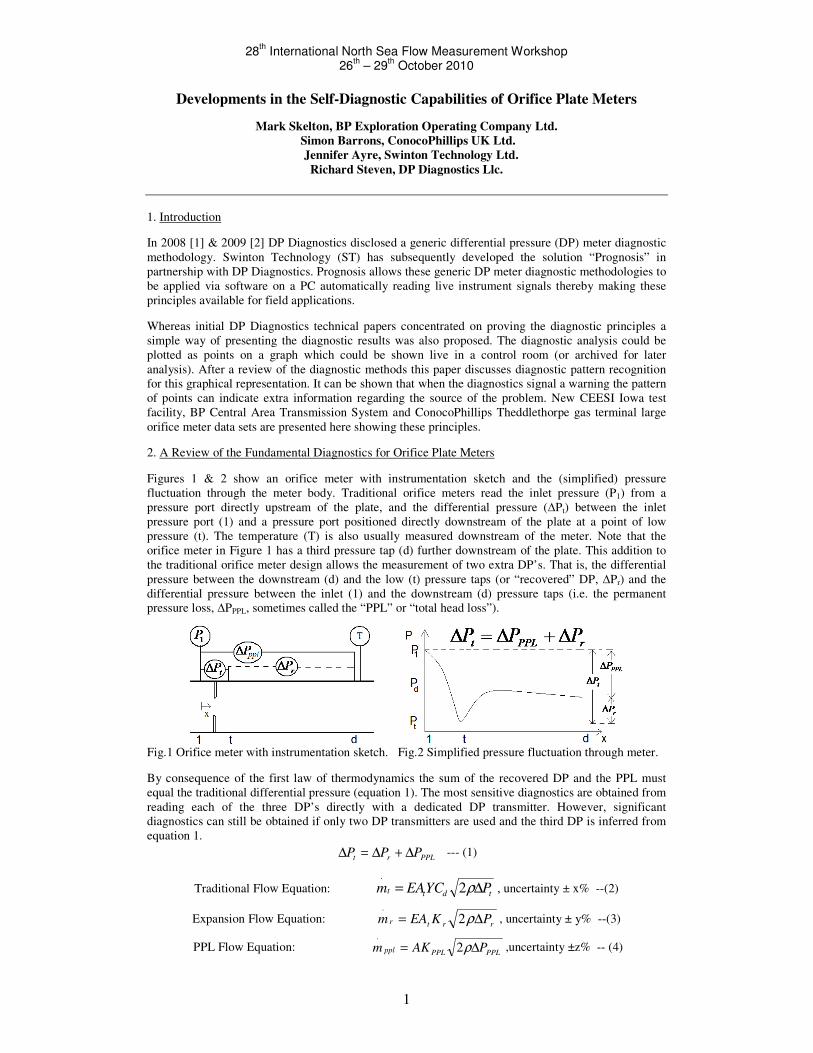
Figures 1 & 2 show an orifice meter with instrumentation sketch and the (simplified) pressure

fluctuation through the meter body. Traditional orifice meters read the inlet pressure (P1) from a

pressure port directly upstream of the plate, and the differential pressure (∆Pt) between the inlet

pressure port (1) and a pressure port positioned directly downstream of the plate at a point of low

pressure (t). The temperature (T) is also usually measured downstream of the meter. Note that the

orifice meter in Figure 1 has a third pressure tap (d) further downstream of the plate. This addition to

the traditional orifice meter design allows the measurement of two extra DP’s. That is, the differential

pressure between the downstream (d) and the low (t) pressure taps (or “recovered” DP, ∆Pr) and the

differential pressure between the inlet (1) and the downstream (d) pressure taps (i.e. the permanent

pressure loss, ∆PPPL, sometimes called the “PPL” or “total head loss”).

Fig.1 Orifice meter with instrumentation sketch. Fig.2 Simplified pressure fluctuation through meter.

By consequence of the first law of thermodynamics the sum of the recovered DP and the PPL must

equal the traditional differential pressure (equation 1). The most sensitive diagnostics are obtained from

reading each of the three DP’s directly with a dedicated DP transmitter. However, significant

diagnostics can still be obtained if only two DP transmitters are used and the third DP is inferred from

equation 1.

PPLrt PPP ∆+∆=∆ --- (1)

Traditional Flow Equation: tdtt PYCEAm ∆= ρ2.

, uncertainty ± x% --(2)

Expansion Flow Equation: rrtr PKEAm ∆= ρ2

.

, uncertainty ± y% --(3)

PPL Flow Equation: PPLPPLppl PAKm ∆= ρ2

.

,uncertainty ±z% -- (4)

28th International North Sea Flow Measurement Workshop

26th – 29

th October 2010

2

The traditional orifice meter flow rate equation is shown here as equation 2. Traditionally, this is the

only DP meter flow rate calculation. However, with the additional downstream pressure tap three flow

equations can be produced. That is, the recovered DP can be used to find the flow rate with an

“expansion” flow equation (see equation 3) and the PPL can be used to find the flow rate with a “PPL”

flow equation (see equation 4). Note that tm.

, rm.

& PPLm.

represents the traditional, expansion and PPL

mass flow rate equation predictions of the actual mass flow rate (.

m ) respectively. The symbol ρ

represents the fluid density. Symbols E , A andtA represent the velocity of approach (a constant for a

set meter geometry), the inlet cross sectional area and the minimum (or “throat”) cross sectional area

through the meter respectively. Y is an expansion factor accounting for gas density fluctuation through

the meter. (For liquids Y =1.) The terms dC ,

rK & PPLK represent the discharge coefficient, the

expansion coefficient and the PPL coefficient respectively. These parameters are usually expressed as

functions of the orifice meter geometry and the flow’s Reynolds number.

Dm πµ.

4Re = --- (5)

The Reynolds number is expressed as equation 5. Note that µ is the fluid viscosity and D is the inlet

diameter. In this case, as the Reynolds number (Re) is flow rate dependent, these flow rate predictions

must be obtained by iterative methods within the Prognosis software. A detailed derivation of these

three flow rate equations is given by Steven [1].

Every orifice meter run is in effect three flow meters. As there are three flow rate equations predicting

the same flow through the same meter body there is the potential to compare the flow rate predictions

and hence have a diagnostic system. Naturally, all three flow rate equations have individual uncertainty

ratings (say x%, y% & z% as shown in equations 2 through 4). Therefore, even if a DP meter is

operating correctly, no two flow predictions would match precisely. However, a correctly operating

meter should have no difference between any two flow equations greater than the sum of the two

uncertainties (and typically no greater than the route mean squared of the two uncertainties). The

system therefore has three more uncertainties, i.e. the maximum allowable difference between any two

flow rate equations, as shown in equation set 6a to 6c. This allows a self diagnosing system. If the

percentage difference between any two flow rate equations is less than that equation pair’s summed

uncertainties, then no potential problem is found and the traditional flow rate prediction can be trusted.

If however, the percentage difference between any two flow rate equations is greater than that equation

pair’s summed uncertainties then this indicates a metering problem and the flow rate predictions should

not be trusted. The three flow rate percentage differences are calculated by equations 7a to 7c.

Traditional & PPL Meters allowable difference ( %φ ): %%% zx +=φ -- (6a)

Traditional & Expansion Meters allowable difference ( %ξ ): %%% yx +=ξ -- (6b)

Expansion & PPL Meters allowable difference ( %υ ): %%% zy +=υ -- (6c)

Traditional to PPL Meter Comparison: %100*%...

−=

tmmm tPPLψ -- (7a)

Traditional to Expansion Meter Comparison: %100*%...

−=

tmmm trλ -- (7b)

PPL to Expansion Meter Comparison: %100*%...

−=

PPLmmm PPLrχ -- (7c)

This diagnostic methodology uses the three individual DP’s to independently predict the flow rate and

then compares these results. In effect, the individual DP’s are therefore being directly compared.

However, it is possible to take a different diagnostic approach. The Pressure Loss Ratio (or “PLR”) is

the ratio of the PPL to the traditional DP. The PLR is almost constant for orifice meters operating with

single phase homogenous flow, as indicated by ISO 5167 [3]. We can rewrite Equation 1:

1=∆

∆+

∆

∆

t

PPL

t

r

P

P

P

P-- (1a) where

t

PPL

P

P

∆

∆

is the PLR.

28th International North Sea Flow Measurement Workshop

26th – 29

th October 2010

3

From equation 1a, if the PLR is a constant set value then both the Pressure Recovery Ratio or “PRR”,

(i.e. the ratio of the recovered DP to traditional DP) and the Recovered DP to PPL Ratio, or “RPR”

must then also be constant set values. That is, all three DP ratios available from the three DP’s read are

effectively constant values for any correctly operating orifice meter. Thus we have:

PPL to Traditional DP ratio (PLR): ( )settPPL PP ∆∆ , uncertainty ± a%

Recovered to Traditional DP ratio (PRR): ( )settr PP ∆∆ , uncertainty ± b%

Recovered to PPL DP ratio (RPR): ( )setPPLr PP ∆∆ , uncertainty ± c%

Here then is another method of using the three DP’s to check an orifice meters health. Actual DP ratios

found in service can be compared to set known correct operational values. Let us denote the difference

between this read (PLRread) and correct (PLRset) operation PLR value asα , the difference between the

read (PRRread) and correct (PRRset) operation PRR value asγ , and the difference between the read

(RPRread) and the correct (RPRset) operation RPR asη . These values are found by equations 8a to 8c.

[ ]{ } %100*/% setsetread PLRPLRPLR −=α --(8a)

[ ]{ } %100*/% setsetread PRRPRRPRR −=γ --(8b)

[ ]{ } %100*/% setsetread RPRRPRRPR −=η --(8c)

It should be noted here that in order to calculate ±ψ %, ± λ , ± χ % and ±α %, ±γ , ±η % the system

requires to know the set (i.e. correct) discharge coefficient, the expansion coefficient, PPL coefficient,

PLR, PRR and RPR values. As orifice plate meters are not calibrated it is necessary to derive these

values from ISO 5167 [3]. ISO states a discharge coefficient prediction in the form of the Reader-

Harris Gallagher (RHG) equation. It should also be noted that ISO 5167 also offers a prediction for the

PLR (see equation 9). From consideration of equation 1a we can then derive associated values for the

PRR & RPR as shown is equations 10 & 11 respectively.

( ){ }( ){ } 224

224

11

11

ββ

ββ

dd

dd

CC

CCPLR

+−−

−−−= -- (9) PLRPRR −= 1 -- (10),

PLR

PRRRPR = -- (11)

Furthermore, it can be shown that from initial standard’s knowledge of the discharge coefficient and

the PLR the expansion and PPL coefficients can be found as shown by equations 12 & 13. Therefore,

from the standard’s discharge coefficient and PLR predictions the expansion coefficient, PPL

coefficient, PRR and RPR can be deduced. Unfortunately, ISO gives no uncertainty value with the PLR

prediction.

PLR

YCK d

r−

=1

--(12) PLR

YCEK d

ppl

2β= --(13) where

A

At=β -- (14)

An orifice meter with a downstream pressure tap can produce six meter parameters with nine

associated uncertainties. These six parameters are the discharge coefficient, expansion flow

coefficient, and PPL coefficient, PLR, PRR and RPR. The nine uncertainties are the six parameter

uncertainties (±x%, ±y%, ±z%, ±a%, ±b% & ±c%) and the three flow rate inter-comparison

uncertainties (±φ %, ±ξ , ±ν %). These fifteen parameters DP meter define the meters correct

operating mode. Any deviation from this mode beyond the acceptable uncertainty limits is an indicator

that there is an orifice meter malfunction and the traditional meter flow rate output is therefore not

trustworthy. Table 1 shows the six possible situations that should signal a warning. Note that each of

the six diagnostic checks has normalized data, i.e. each meter diagnostic parameter output is divided by

the allowable difference for that parameter.

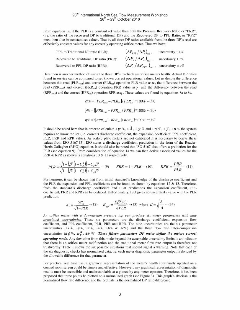
For practical real time use, a graphical representation of the meter’s health continually updated on a

control room screen could be simple and effective. However, any graphical representation of diagnostic

results must be accessible and understandable at a glance by any meter operator. Therefore, it has been

proposed that three points be plotted on a normalized graph (see Figure 3). This graph’s abscissa is the

normalized flow rate difference and the ordinate is the normalized DP ratio difference.

28th International North Sea Flow Measurement Workshop

26th – 29

th October 2010

4

Table 1 The diagnostic analysis Fig.3 A NDB with normalized diagnostic result.

These normalized values have no units. On this graph a normalized diagnostic box (or “NDB”) can be

superimposed with corner co-ordinates: (1,1), (1, 1− ), ( 1− , 1− ) & ( 1− ,1). On such a graph three

meter diagnostic points can be plotted, i.e. ( φψ , aα ), ( ξλ , bγ ) & ( υχ , cη ). That is, the

three DP’s have been split into three DP pairs and for each DP pair the difference in the two flow rate

predictions and, separately, the difference in the actual to set DP ratio are being compared to their

maximum allowable differences. If all points are within or on the NDB (as shown in Figure 3) the

meter operator sees no metering problem and the traditional meter’s flow rate prediction can be trusted.

However, if one or more of the three points falls outside the NDB the meter operator has a visual

indication that the meter is not operating correctly and that the meter’s traditional (or any) flow rate

prediction cannot be trusted. Furthermore, when a problem is indicated further analysis of the

diagnostics can result in further information being learned regarding the nature of the problem.

3. Measurement Issues with the Three Differential Pressures

3a. Three DP Transmitters vs. Two DP Transmitters

Equation 1 is a consequence of the first law of thermodynamics and therefore it cannot be violated.

Equation 1 is the most fundamental diagnostic check for orifice meters that utilise three DP transmitters

to independently read the traditional DP, the recovered DP and the PPL. The sum of the read recovered

DP (of uncertainty q%) and read PPL (of uncertainty r%) must equate to the read traditional DP (of

uncertainty p%) within the uncertainty ranges of the DP transmitters. (See equation 1b.)

( ) ( ) ( )%%% rPqPpP PPLrt ±∆+±∆=±∆ --- (1b)

If the three read DP’s do not agree with equation 1b then this is an indication that one or more of the

DP measurements are incorrect. Common physical orifice meter problems such as damaged,

contaminated or incorrectly installed plates, wet gas flows or incorrect geometry keypad entries do not

cause the actual DP’s to disobey equation 1. The real DP’s created in the flow by the meter must follow

the laws of physics regardless of whether the meter is predicting the actual flow rate or not and

regardless of whether the instruments are reading the correct DP values or not. Hence, if equation 1b

appears not to hold then there is a problem with the measurements of one or more of the DP’s being

created. Such an instrument problem must be attended to before any further analysis regarding the

physical performance of the orifice meter is made.

Note that this very simple but powerful diagnostic check is only available if the meter operator chooses

to use three DP transmitters (i.e. an extra two DP transmitters). An operator may decide on the simpler

and less expensive option of adding just one extra DP transmitter and inferring the third DP from

equation 1. However, in this case this very simple diagnostic check will not be available. Furthermore,

it will be shown that the option of using two DP transmitters instead of three also reduces the

diagnostic system’s overall capability. Nevertheless, as will be seen, this simpler option still allows

some valuable diagnostic analysis on the orifice meter’s performance.

3b A Comment on the Use of Two DP Transmitters Only

If only one extra DP transmitter is to be utilised to produce orifice meter diagnostics it is the smaller

recovered DP that should be directly read and the larger PPL should be inferred by equation 1. This

arrangement may not be immediately apparent to flow meter technicians who are used to reading the

traditional DP and occasionally the PPL (for system hydraulic loss calculations.) This preference is due

28th International North Sea Flow Measurement Workshop

26th – 29

th October 2010

5

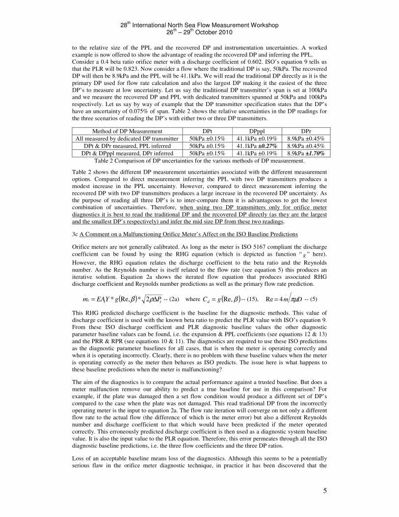
to the relative size of the PPL and the recovered DP and instrumentation uncertainties. A worked

example is now offered to show the advantage of reading the recovered DP and inferring the PPL.

Consider a 0.4 beta ratio orifice meter with a discharge coefficient of 0.602. ISO’s equation 9 tells us

that the PLR will be 0.823. Now consider a flow where the traditional DP is say, 50kPa. The recovered

DP will then be 8.9kPa and the PPL will be 41.1kPa. We will read the traditional DP directly as it is the

primary DP used for flow rate calculation and also the largest DP making it the easiest of the three

DP’s to measure at low uncertainty. Let us say the traditional DP transmitter’s span is set at 100kPa

and we measure the recovered DP and PPL with dedicated transmitters spanned at 50kPa and 100kPa

respectively. Let us say by way of example that the DP transmitter specification states that the DP’s

have an uncertainty of 0.075% of span. Table 2 shows the relative uncertainties in the DP readings for

the three scenarios of reading the DP’s with either two or three DP transmitters.

Method of DP Measurement DPt DPppl DPr

All measured by dedicated DP transmitter 50kPa ±0.15% 41.1kPa ±0.19% 8.9kPa ±0.45%

DPt & DPr measured, PPL inferred 50kPa ±0.15% 41.1kPa ±0.27% 8.9kPa ±0.45%

DPt & DPppl measured, DPr inferred 50kPa ±0.15% 41.1kPa ±0.19% 8.9kPa ±1.70%

Table 2 Comparison of DP uncertainties for the various methods of DP measurement.

Table 2 shows the different DP measurement uncertainties associated with the different measurement

options. Compared to direct measurement inferring the PPL with two DP transmitters produces a

modest increase in the PPL uncertainty. However, compared to direct measurement inferring the

recovered DP with two DP transmitters produces a large increase in the recovered DP uncertainty. As

the purpose of reading all three DP’s is to inter-compare them it is advantageous to get the lowest

combination of uncertainties. Therefore, when using two DP transmitters only for orifice meter

diagnostics it is best to read the traditional DP and the recovered DP directly (as they are the largest

and the smallest DP’s respectively) and infer the mid size DP from these two readings.

3c A Comment on a Malfunctioning Orifice Meter’s Affect on the ISO Baseline Predictions

Orifice meters are not generally calibrated. As long as the meter is ISO 5167 compliant the discharge

coefficient can be found by using the RHG equation (which is depicted as function “ g ” here).

However, the RHG equation relates the discharge coefficient to the beta ratio and the Reynolds

number. As the Reynolds number is itself related to the flow rate (see equation 5) this produces an

iterative solution. Equation 2a shows the iterated flow equation that produces associated RHG

discharge coefficient and Reynolds number predictions as well as the primary flow rate prediction.

( )ttt PgYEAm ∆= ρβ 2*Re,*

.

-- (2a) where

( )βRe,gCd = -- (15),

Dm πµ.

4Re = -- (5)

This RHG predicted discharge coefficient is the baseline for the diagnostic methods. This value of

discharge coefficient is used with the known beta ratio to predict the PLR value with ISO’s equation 9.

From these ISO discharge coefficient and PLR diagnostic baseline values the other diagnostic

parameter baseline values can be found, i.e. the expansion & PPL coefficients (see equations 12 & 13)

and the PRR & RPR (see equations 10 & 11). The diagnostics are required to use these ISO predictions

as the diagnostic parameter baselines for all cases, that is when the meter is operating correctly and

when it is operating incorrectly. Clearly, there is no problem with these baseline values when the meter

is operating correctly as the meter then behaves as ISO predicts. The issue here is what happens to

these baseline predictions when the meter is malfunctioning?

The aim of the diagnostics is to compare the actual performance against a trusted baseline. But does a

meter malfunction remove our ability to predict a true baseline for use in this comparison? For

example, if the plate was damaged then a set flow condition would produce a different set of DP’s

compared to the case when the plate was not damaged. This read traditional DP from the incorrectly

operating meter is the input to equation 2a. The flow rate iteration will converge on not only a different

flow rate to the actual flow (the difference of which is the meter error) but also a different Reynolds

number and discharge coefficient to that which would have been predicted if the meter operated

correctly. This erroneously predicted discharge coefficient is then used as a diagnostic system baseline

value. It is also the input value to the PLR equation. Therefore, this error permeates through all the ISO

diagnostic baseline predictions, i.e. the three flow coefficients and the three DP ratios.

Loss of an acceptable baseline means loss of the diagnostics. Although this seems to be a potentially

serious flaw in the orifice meter diagnostic technique, in practice it has been discovered that the

28th International North Sea Flow Measurement Workshop

26th – 29

th October 2010

6

inherent errors in the baseline values are of no significant consequence. The reason for this is due to the

fact that the RHG discharge coefficient prediction is actually rather insensitive to the Reynolds number.

It takes very large changes in the Reynolds number to produce very small changes in the RHG

discharge coefficient prediction. It has been found that even very considerable meter malfunctions that

produce large flow rate (and therefore Reynolds number) errors shift all the ISO baseline parameter

predictions by an order of magnitude less than the correctly operating meter’s baseline parameters

stated uncertainties. Therefore, we can practically trust the ISO predictions to be applicable as a

useable diagnostic baseline even on a seriously malfunctioning meter.

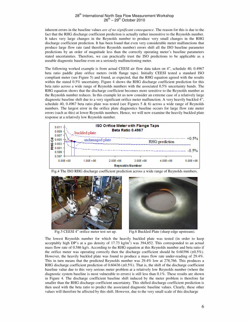
The following worked example is from actual CEESI air flow data taken on 4”, schedule 40, 0.4967

beta ratio paddle plate orifice meters (with flange taps). Initially CEESI tested a standard ISO

compliant meter (see Figure 5) and found, as expected, that the RHG equation agreed with the results

within the stated 0.5% uncertainty. Figure 4 shows the RHG discharge coefficient prediction for this

beta ratio across a wide range of Reynolds numbers with the associated 0.5% uncertainty bands. The

RHG equation shows that the discharge coefficient becomes more sensitive to the Reynolds number as

the Reynolds number reduces. In this example let us now consider an extreme case of a relatively large

diagnostic baseline shift due to a very significant orifice meter malfunction. A very heavily buckled 4”,

schedule 40, 0.4967 beta ratio plate was tested (see Figures 5 & 6) across a wide range of Reynolds

numbers. The largest error in the orifice plate diagnostics baseline occurs for large flow rate meter

errors (such as this) at lower Reynolds numbers. Hence, we will now examine the heavily buckled plate

response at a relatively low Reynolds number.

Fig.4 The ISO RHG discharge coefficient prediction across a wide range of Reynolds numbers.

Fig.5 CEESI 4” orifice meter test set up. Fig.6 Buckled Plate (sharp edge upstream).

The lowest Reynolds number for which the heavily buckled plate was tested (in order to keep

acceptably high DP’s at a gas density of 17.73 kg/m3) was 394,852. This corresponded to an actual

mass flow rate of 0.586 kg/s. According to the RHG equation at this Reynolds number and beta ratio if

the orifice meter was operating correctly then the discharge coefficient should be 0.60396 (±0.5%).

However, the heavily buckled plate was found to produce a mass flow rate under-reading of 29.4%.

This in turn means that the predicted Reynolds number was 29.4% low at 278,766. This produces a

RHG discharge coefficient prediction of 0.60436 (±0.5%). That is, the shift of the discharge coefficient

baseline value due to this very serious meter problem at a relatively low Reynolds number (where the

diagnostic system baseline is most vulnerable to errors) is still less than 0.1%. These results are shown

in Figure 4. The discharge coefficient baseline shift induced by the meter problem is therefore far

smaller than the RHG discharge coefficient uncertainty. This shifted discharge coefficient prediction is

then used with the beta ratio to predict the associated diagnostic baseline values. Clearly, these other

values will therefore be affected by this shift. However, due to the very small scale of this discharge

28th International North Sea Flow Measurement Workshop

26th – 29

th October 2010

7

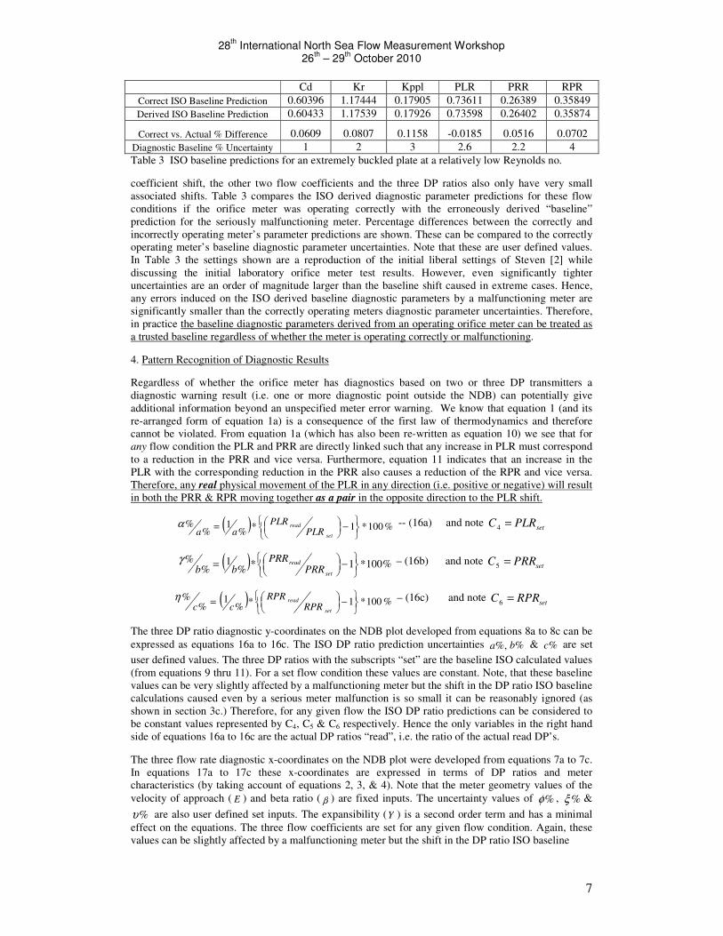
Cd Kr Kppl PLR PRR RPR

Correct ISO Baseline Prediction 0.60396 1.17444 0.17905 0.73611 0.26389 0.35849

Derived ISO Baseline Prediction 0.60433 1.17539 0.17926 0.73598 0.26402 0.35874

Correct vs. Actual % Difference 0.0609 0.0807 0.1158 -0.0185 0.0516 0.0702

Diagnostic Baseline % Uncertainty 1 2 3 2.6 2.2 4

Table 3 ISO baseline predictions for an extremely buckled plate at a relatively low Reynolds no.

coefficient shift, the other two flow coefficients and the three DP ratios also only have very small

associated shifts. Table 3 compares the ISO derived diagnostic parameter predictions for these flow

conditions if the orifice meter was operating correctly with the erroneously derived “baseline”

prediction for the seriously malfunctioning meter. Percentage differences between the correctly and

incorrectly operating meter’s parameter predictions are shown. These can be compared to the correctly

operating meter’s baseline diagnostic parameter uncertainties. Note that these are user defined values.

In Table 3 the settings shown are a reproduction of the initial liberal settings of Steven [2] while

discussing the initial laboratory orifice meter test results. However, even significantly tighter

uncertainties are an order of magnitude larger than the baseline shift caused in extreme cases. Hence,

any errors induced on the ISO derived baseline diagnostic parameters by a malfunctioning meter are

significantly smaller than the correctly operating meters diagnostic parameter uncertainties. Therefore,

in practice the baseline diagnostic parameters derived from an operating orifice meter can be treated as

a trusted baseline regardless of whether the meter is operating correctly or malfunctioning.

4. Pattern Recognition of Diagnostic Results

Regardless of whether the orifice meter has diagnostics based on two or three DP transmitters a

diagnostic warning result (i.e. one or more diagnostic point outside the NDB) can potentially give

additional information beyond an unspecified meter error warning. We know that equation 1 (and its

re-arranged form of equation 1a) is a consequence of the first law of thermodynamics and therefore

cannot be violated. From equation 1a (which has also been re-written as equation 10) we see that for

any flow condition the PLR and PRR are directly linked such that any increase in PLR must correspond

to a reduction in the PRR and vice versa. Furthermore, equation 11 indicates that an increase in the

PLR with the corresponding reduction in the PRR also causes a reduction of the RPR and vice versa.

Therefore, any real physical movement of the PLR in any direction (i.e. positive or negative) will result

in both the PRR & RPR moving together as a pair in the opposite direction to the PLR shift.

( ) %100*1*%

1%

%

−

=

set

read

PLRPLR

aaα

-- (16a) and note

setPLRC =4

( ) %100*1*%

1%

%

−

=

set

read

PRRPRR

bbγ

– (16b) and note

setPRRC =5

( ) %100*1*%

1%

%

−

=

set

read

RPRRPR

ccη

– (16c) and note

setRPRC =6

The three DP ratio diagnostic y-coordinates on the NDB plot developed from equations 8a to 8c can be

expressed as equations 16a to 16c. The ISO DP ratio prediction uncertainties %,a %b & %c are set

user defined values. The three DP ratios with the subscripts “set” are the baseline ISO calculated values

(from equations 9 thru 11). For a set flow condition these values are constant. Note, that these baseline

values can be very slightly affected by a malfunctioning meter but the shift in the DP ratio ISO baseline

calculations caused even by a serious meter malfunction is so small it can be reasonably ignored (as

shown in section 3c.) Therefore, for any given flow the ISO DP ratio predictions can be considered to

be constant values represented by C4, C5 & C6 respectively. Hence the only variables in the right hand

side of equations 16a to 16c are the actual DP ratios “read”, i.e. the ratio of the actual read DP’s.

The three flow rate diagnostic x-coordinates on the NDB plot were developed from equations 7a to 7c.

In equations 17a to 17c these x-coordinates are expressed in terms of DP ratios and meter

characteristics (by taking account of equations 2, 3, & 4). Note that the meter geometry values of the

velocity of approach ( E ) and beta ratio ( β ) are fixed inputs. The uncertainty values of %φ , %ξ &

%υ are also user defined set inputs. The expansibility (Y ) is a second order term and has a minimal

effect on the equations. The three flow coefficients are set for any given flow condition. Again, these

values can be slightly affected by a malfunctioning meter but the shift in the DP ratio ISO baseline

28th International North Sea Flow Measurement Workshop

26th – 29

th October 2010

8

%100*1%

1%

%2

−

= read

d

PPL PLRYCE

K

βφφψ --(17a) and note

≈

d

PPL

YCE

KC

21β

--(18a)

%100*1%

1%

%

−

= read

d

r PRRYC

K

ξξλ --(17b) and note

≈

d

r

YC

KC2

--(18b)

( ) %100*1%

1%

%2

−

= read

PPL

r RPRK

KEβυυ

χ --(17c)

and note

≈

PPL

r

K

KEC

2

3

β --(18c)

calculations caused even by a serious meter malfunction is so small it can be reasonably ignored (as

shown in section 3c.) Therefore groups of terms in equations 17a to 17c are effectively constant values

as shown in equation 18a to 18c. Therefore, the diagnostic checks have been reduced to a set of

constants used with the three “read” DP ratios. That is, the diagnostic coordinates plotted with the NDB

can be expressed in terms of DP ratios only. Let us denote the traditional DP to PPL diagnostic check

as “point 1”, the traditional to recovered DP diagnostic check as “point 2” and the recovered DP to PPL

diagnostic check as “point 3”. Therefore, we can express each of the three points in the following way:

“Point 1”, i.e.

%

%,

%

%

a

α

φ

ψ , is ( ){ } ( ){ }

−−%100*

%

1,%100*

%

141

a

CPLRPLRCreadread

φ

“Point 2”, i.e.

%

%,

%

%

b

γ

ξ

λ , is ( ){ } ( ){ }

−−%100*

%

1,%100*

%

152

b

CPRRPRRCreadread

ξ

“Point 3”, i.e.

%

%,

%

%

c

η

υ

χ, is ( ){ } ( ){ }

−−%100*

%

1,%100*

%

163

c

CRPRRPRCreadread

υ

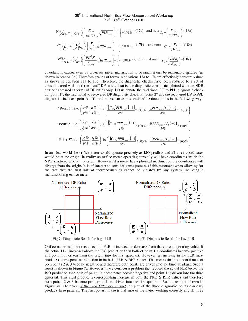
In an ideal world the orifice meter would operate precisely as ISO predicts and all three coordinates

would be at the origin. In reality an orifice meter operating correctly will have coordinates inside the

NDB scattered around the origin. However, if a meter has a physical malfunction the coordinates will

diverge from the origin. It is of interest to consider consequences of this statement when allowing for

the fact that the first law of thermodynamics cannot be violated by any system, including a

malfunctioning orifice meter.

Fig.7a Diagnostic Result for high PLR. Fig.7b Diagnostic Result for low PLR.

Orifice meter malfunctions cause the PLR to increase or decrease from the correct operating value. If

the actual PLR increases above the ISO prediction then both of point 1’s coordinates become positive

and point 1 is driven from the origin into the first quadrant. However, an increase in the PLR must

produce a corresponding reduction in both the PRR & RPR values. This means that both coordinates of

both points 2 & 3 become negative and therefore both points are driven into the third quadrant. Such a

result is shown in Figure 7a. However, if we consider a problem that reduces the actual PLR below the

ISO prediction then both of point 1’s coordinates become negative and point 1 is driven into the third

quadrant. This must produce a corresponding increase in both the PRR & RPR values and therefore

both points 2 & 3 become positive and are driven into the first quadrant. Such a result is shown in

Figure 7b. Therefore, if the read DP’s are correct the plot of the three diagnostic points can only

produce three patterns. The first pattern is the trivial case of the meter working correctly and all three

28th International North Sea Flow Measurement Workshop

26th – 29

th October 2010

9

diagnostic points inside the NDB (see Figure 3). In this case the points can be randomly distributed

inside the box (and the four quadrants) as uncertainty in the data allows for the point to fall around the

origin. The second pattern is the case where a physical problem has caused an increase in the PLR

above the standard operating value (Figure 7a). The third pattern is the case where a physical problem

has caused a decrease in the PLR below the standard operating value (Figure 7b). Note that this pattern

discussion relates to the graph and its quadrants, and not directly to the NDB superimposed on it. A

diagnostic warning is given even if only one of the three points is outside the NDB. However, even

here one of these two general patterns must be seen, even with two of the points inside the NDB.

There are three diagnostic points to be placed somewhere on the four quadrants of the diagnostic graph.

That means there are 64 different mathematical combinations of diagnostic patterns, i.e. four possible

positions to the power of three diagnostic points. However, as we have seen, when one or more of the

three diagnostic points fall outside the NDB, from physical restrictions only two of these sixty four

patterns can be created by an orifice meter with a physical problem when reading the DP’s correctly. Any one of the other sixty two patterns contravenes the first law of thermodynamics.

Therefore, as it is not physically possible to violate this law, any diagnostic warning result that is not

one of the two patterns discussed above indicates that there must be a problem with the DP

measurements. If the system does not measure the DP’s correctly then the read DP’s being supplied to

the diagnostic system are erroneous and therefore, unlike the actual DP’s being produced by a

functioning or malfunctioning meter, they are not bound by the physical laws. That is, if one or more

DP transmitters have a problem due to drift, saturation, a blocked impulse line, a poor calibration, a

leaking manifold valve etc. then its output can have any random error. Therefore such erroneous

instrument readings do not have to be related to the physical reality of what DP’s are really being

created by the flow through either a correctly operating orifice meter or an orifice meter with a physical

problem. That is, faulty instrumentation can give readings that make no physical sense. Random DP

transmitter errors will produce random diagnostic patterns. Hence, a diagnostic pattern that is different

to the two patterns allowed by the physical laws indicates a DP measurement problem.

DP reading errors can produce any of the sixty four diagnostic patterns. Sixty two of these directly

indicate to the operator a DP reading problem. However, it should be noted here that while these sixty

two diagnostic patterns guarantee that there is a DP reading problem it does not guarantee that this is

the only problem. There could be both DP reading problems and physical problems with the meter.

However, the operator will know for sure that a first step in fixing the meter is to fix the DP readings.

(Once this is done the diagnostic pattern either falls inside the NDB for correct operation, or into one of

the two patterns that are created by a physical problem.) It should also be noted that as DP reading

errors can produce any combination of DP’s they can produce any of the sixty four warning patterns.

Therefore, if one of the two patterns that can be created by a physical meter problem exists this does

not exclude the meters problem being due DP reading errors. However, if three DP transmitters are in

use an immediate simple DP check for any warning pattern is equation 1b. Finally, on that issue it

should be noted that DP reading error issues are clearer if the operator chooses to use three dedicated

transmitters instead of two. If the system has three DP transmitters then both equation 1b and the

resulting diagnostic plot can tell operator a lot about the DP reading error. If the system only has two

DP transmitters then it is more difficult to isolate a DP reading problem. Naturally, with more expense

and complexity comes more capability. Field data will be shown in sections 7 & 8 where the diagnostic

results will be related to these discussions.

A further experimental observation can be made. It appears that for a fully developed flow into an

orifice meter with a physical problem (as opposed to an instrument problem) Figure 7a represents a

positive flow rate prediction bias and Figure 7b represents a negative flow rate prediction bias. Note

however, that this observation excludes the problems caused by disturbed flow profiles introduced by

non-standard orifice meter installation, partially blocked upstream conditioning plates or debris from

damaged upstream components in front of the plate etc... At the time of writing a technical proof of this

result has not been successfully developed. However, with the exception of disturbed inlet flow

profiles, multiple diagnostic tests on a wide range of common physical orifice meter problems, carried

out over three years on five different test facility and field locations, have failed to produce one single

physical problem which contradicts this observation.

Finally, note that keeping the diagnostic points inside a NDB requires a precise flow meter response.

When the meter uncertainties (±x%, ±y%, ±z%, ±a%, ±b% & ±c%) are set at the lowest realistic values

then inside the NDB represents a small window of allowable meter performance variation. This is the

basis for why the diagnostics are so sensitive to so many problems. Hence, it is highly unlikely that a

28th International North Sea Flow Measurement Workshop

26th – 29

th October 2010

10

malfunctioning meter could have two problems that precisely counter each other such that the points

remained inside the small precise performance range of the NDB.

5. Non-Standard Orifice Plate Meter Installations

5a. Downstream Pressure Tap > 6D

Operators of orifice meters already in service could benefit from having them made diagnostic capable.

However, to have orifice meter diagnostics a downstream tap must be available. New systems can be

built with a pressure tap at 6D downstream from the plate (as dictated by ISO 5167) and with the

thermo well downstream of this tap. ISO 5167 states that the thermo well shall be between 5D & 15D

downstream of the plate. However, existing installations often do not have a downstream pressure tap

available at 6D from the plate and furthermore the thermo well can be located in this vicinity.

Therefore, to retrofit many existing orifice meters with diagnostics would mean using a downstream

pressure tap located further downstream from the plate than 6D and possibly downstream of

components such as thermo wells. This extra length of pipe and the extra components add to the

system’s permanent pressure loss making the read PPL higher and the recovered DP lower than the

ISO based predictions. In turn this produces a bias on the diagnostic parameter baselines. Naturally

with the extra permanent pressure loss being compared to the standard traditional DP this increases the

PLR above the ISO prediction (which is based on the 6D downstream pressure tap location). Therefore

the bias on the diagnostic system sets the result for a correctly operating orifice meter as shown in

Figure 7a. Whereas this situation is not ideal it does not prohibit the addition of diagnostics to such an

existing system. It is possible to introduce a modification factor which “zeros” the diagnostic points to

the origin thereby giving a correct diagnostic baseline for a correctly operating meter. Such retrofits

could be considered on many currently installed orifice meter installations. It is therefore now derived.

The term DL is the distance between the actual downstream pressure port and a port at 6D divided by

the inside bore diameter (i.e. 6−= nDL .) The friction factor “ f ” is pipe relative roughness

dependent and is also related to the Reynolds number, as shown in the Moody diagram (presented in

most Fluid Mechanics text books). Most industrial flow ranges have Reynolds numbers considerably

greater than 100,000 and for pipe that would typically be used downstream of an orifice meter the

relative roughness (Ra/D) is usually 0.00005 ≤ Ra/D ≤ 0.0015. Under these flow conditions the friction

factor is effectively independent of the Reynolds number and therefore a constant keypad entry offers

enough accuracy for the diagnostic system modification factor. Kloss is the loss coefficient for the

length of pipe between 6D & nD. Kl,minor is the minor loss coefficient for a pipe component installed

between 6D & nD.

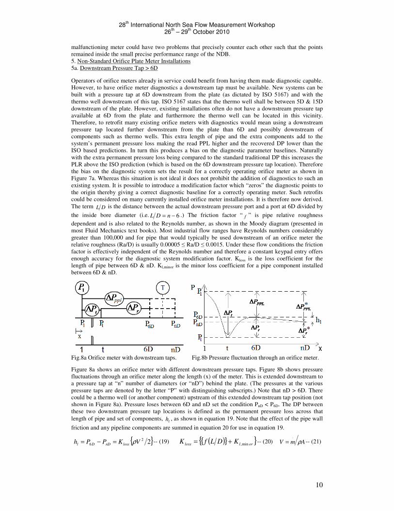
Fig.8a Orifice meter with downstream taps. Fig.8b Pressure fluctuation through an orifice meter.

Figure 8a shows an orifice meter with different downstream pressure taps. Figure 8b shows pressure

fluctuations through an orifice meter along the length (x) of the meter. This is extended downstream to

a pressure tap at “n” number of diameters (or “nD”) behind the plate. (The pressures at the various

pressure taps are denoted by the letter “P” with distinguishing subscripts.) Note that nD > 6D. There

could be a thermo well (or another component) upstream of this extended downstream tap position (not

shown in Figure 8a). Pressure loses between 6D and nD set the condition PnD < P6D. The DP between

these two downstream pressure tap locations is defined as the permanent pressure loss across that

length of pipe and set of components, lh , as shown in equation 19. Note that the effect of the pipe wall

friction and any pipeline components are summed in equation 20 for use in equation 19.

{ }22

6 VKPPh lossnDDl ρ=−= -- (19) ( ){ }{ }orlloss KDLfK min,+= -- (20) AmV ρ.

= -- (21)

28th International North Sea Flow Measurement Workshop

26th – 29

th October 2010

11

The term “V ” in equation 19 represents the fluid velocity at the inlet to the meter. Equation 21 shows

the mass continuity equation expressing this velocity in terms of the mass flow rate (.

m ), fluid

density ( ρ ) and meter inlet area ( A ). The inlet diameter (and therefore the inlet area) and the fluid

density are keypad entries. The diagnostic system can utilise the mass flow rate found by the traditional

orifice meter flow rate prediction, i.e. equation 2, to find the inlet velocity. Hence the extra permanent

pressure loss can be predicted and a modification factor applied. Figure 8b shows the relationship between the permanent pressure loss at 6D (

PPLP∆ ) and at the extended

length of nD ( *

PPLP∆ ). It is expressed as equation 22. Figure 8b also shows the relationship of the

recovered DP at 6D (rP∆ ) and at the extended length of nD ( *

rP∆ ). It is expressed as equation 23. The

traditional DP (tP∆ ) remains unaffected. It is related to the DP’s at 6D and nD through equation 24.

The “read” DP ratios (denoted with superscript “*”) as expressed by equations 25 to 27 are for a

downstream tap at nD.

lPPLPPL hPP +∆=∆ * -- (22) lrr hPP −∆=∆ *

-- (23)

( ) ( )lrlPPLrPPLrPPLt hPhPPPPPP −∆++∆=∆+∆=∆+∆=∆ ** -- (24)

t

PPL

P

PPLR

∆

∆=

**

-- (25)

t

r

P

PPRR

∆

∆=

**

-- (26) *

*

*

**

PLR

PRR

P

PRPR

PPL

r =∆

∆= -- (27)

Relationships can be found between the “read” and ISO DP ratios predictions by considering the

definitions of the DP ratios and applying equation 22 thru 26. These relationships are shown as

equations 28 to 30. These relationships convert the ISO DP ratio predictions for a downstream tap at

6D into an equivalent prediction at nD. That is, the baseline DP ratios to be used with an orifice meter

with an extended downstream pressure tap must be found from equations 28 to 30.

t

l

t

l

t

PPL

t

PPL

P

hPLR

P

h

P

P

P

PPLR

∆+=

∆+

∆

∆=

∆

∆=

**

-- (28)

t

l

t

l

t

r

t

r

P

hPRR

P

h

P

P

P

PPRR

∆−=

∆−

∆

∆=

∆

∆=

**

-- (29) *

**

PLR

PRRRPR = -- (30)

The traditional meter is unaffected by the downstream pressure tap location. Therefore the discharge

coefficient does not need to be modified. This is not so for the expansion & PPL flow meters. As they

use the measured recovered DP and PPL to predict the flow rate respectively, a pressure tap further

downstream than 6D will produce different DP’s and this of course affects the flow rate predictions. An

unmodified expansion meter equation would under-read the flow and an unmodified PPL equation

would over read the flow. Modifications for the expansion and PPL flow coefficients are now derived.

Expansion Flow Equation: **

.

22 rrtrrtr PKEAPKEAm ∆=∆= ρρ --(3a)

PPL Flow Equation: **.

22 PPLPPLPPLPPLppl PAKPAKm ∆=∆= ρρ -- (4a)

**

*

*

* 1r

l

r

r

lr

r

r

r

rrP

hK

P

hPK

P

PKK

∆+=

∆

+∆=

∆

∆=

-- (3b)

**

*

*

*1

PPL

l

PPL

PPL

lPPL

PPL

PPL

PPL

PPLPPLP

hK

P

hPK

P

PKK

∆−=

∆

−∆=

∆

∆=

-- (4b)

Equation 3a shows the standard and modified expansion equation for the case of the extended

downstream pressure tap. Here a modified expansion flow coefficient ( *

rK ) is introduced. Equation 3a

can be further reduced to equation 3b. Equation 4a shows the standard and modified PPL equation for

the case of the extended downstream pressure tap. Here a modified PPL flow coefficient ( *

PPLK ) is

28th International North Sea Flow Measurement Workshop

26th – 29

th October 2010

12

introduced. Equation 4a can be further reduced to equation 4b. For orifice meter installations with a

pressure tap further downstream than 6D from the plate these modified expansion and PPL coefficients

must be used in place of the standard flow coefficients used for pressure taps at 6D.

Consider such a case where a pressure tap is at an extended distance downstream (i.e. > 6D). When the

meter is serviceable the modifications to the baseline parameters are applied and the baseline therefore

remains valid. It now may be asked if these calculated modified baseline parameters remain valid when

the meter malfunctions and the flow rate prediction is incorrect. These modified baseline parameters

will only remain valid if they are effectively independent of a malfunctioning meter’s mass flow

prediction and its associated DP’s. It can be shown that this is in fact the case.

Equation 19a shows equation 19 with the mass continuity (i.e. equation 21) and the traditional orifice

meter flow rate prediction calculation (i.e. equation 2) substituted in. Therefore equation 19b shows

that the extra head loss to traditional DP ratio can be reduced to an expression where none of the terms

are sensitive to a meter malfunction. That is the velocity of approach (E) and the beta ratio (β) are set

geometry values. The loss coefficient (lossK ) is only related to the flow rate prediction through the

friction factor’s dependency on the Reynolds number; however this could be described as a second

order effect at most. Likewise the gas expansibility factor and discharge coefficient prediction are

related to the read differential pressure and the predicted Reynolds number respectively but only in a

very insensitive way. Again, these are second order effects. Equations 31 and 32 show the baseline

modification parameters for the expansion coefficient and the PPL coefficient respectively. The only

additional terms to those used in equation 19b are the ISO predicted PRR & PLR terms. Equations 9 &

10 show that these are only related to the orifice meter’s beta ratio and the Reynolds number. Again, as

the beta ratio is a set geometric value and the discharge coefficient is only very mildly sensitive to the

Reynolds number, these terms are also effectively independent of the meter’s flow rate prediction and

associated DP’s. In effect then, the diagnostics baseline parameter modification method for an extended

downstream pressure tap location can be considered from a practical stand point independent of

whether the meter is operating correctly or malfunctioning. Therefore, for orifice meters with

downstream taps located further downstream than 6D, any errors in the modified diagnostic parameter

baselines induced by a meter malfunction are very small and can reasonably be regarded as

insignificant.

( ) ( )tdloss

tdtlosslosslossl PEYCK

A

PYCEAK

A

mK

VKh ∆=

∆=

== ...

2

2..

2.

2.. 42

2

2

2.

2

βρ

ρ

ρ

ρρ -- (19a)

( ) 42.. βdloss

t

l EYCKP

h=

∆ --(19b)

( )( ){ }42

42

*..

..

β

β

dloss

dloss

r

l

EYCKPRR

EYCK

P

h

−=

∆ --(31)

( )( ){ }42

42

*..

..

β

β

dloss

dloss

PPL

l

EYCKPLR

EYCK

P

h

+=

∆ -- (32)

5b. A Generalised Zeroing Factor

In rare cases it may be found that the available pressure tap is closer to the plate than 6D. This is a

more difficult scenario as the recovery of the pressure is incomplete and the recovery path of the

pressure is undefined. However, it is possible to still “zero” the diagnostics by using a generic zeroing

technique (wholly analogous with the technique used for the extended downstream pressure tap). Such

a technique can also be used in other circumstances. For example for a meter known to have a problem

that may affect performance, but the pipeline continues in service until scheduled maintenance, there

may be a desire to monitor any further changes in the meter’s performance. In order to clearly see any

shifting performance over time it is useful to zero out any initial existing bias shown on the NDB plot.

The zeroing technique simply requires the meter operator to input a single correction factor to the

software. This correction factor is denoted here as “Z”. The derivation of this technique is now given.

Figure 9a represents a generic orifice meter. The plate may be installed incorrectly (such as backwards

or not centred). In service the plate may be damaged (e.g. buckled, worn edge, contaminated etc.). The

flow may be two phase flow. The downstream pressure tap may be located at <6D. The downstream

tap may have a small bled flow rate to a densitometer affecting the pressure reading. The recovered DP

or PPL transmitter may have been found to have drifted. All these scenarios (and many more) cause the

read pressure field through the orifice meter to change from the expected ISO baseline. Figure 9b

28th International North Sea Flow Measurement Workshop

26th – 29

th October 2010

13

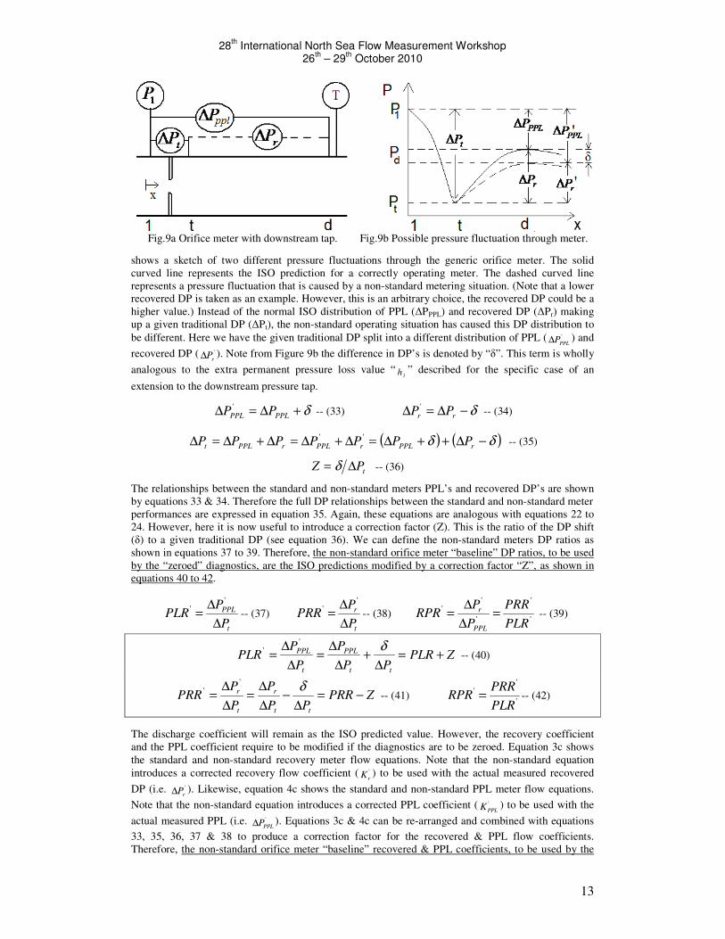
Fig.9a Orifice meter with downstream tap. Fig.9b Possible pressure fluctuation through meter.

shows a sketch of two different pressure fluctuations through the generic orifice meter. The solid

curved line represents the ISO prediction for a correctly operating meter. The dashed curved line

represents a pressure fluctuation that is caused by a non-standard metering situation. (Note that a lower

recovered DP is taken as an example. However, this is an arbitrary choice, the recovered DP could be a

higher value.) Instead of the normal ISO distribution of PPL (∆PPPL) and recovered DP (∆Pr) making

up a given traditional DP (∆Pt), the non-standard operating situation has caused this DP distribution to

be different. Here we have the given traditional DP split into a different distribution of PPL ( '

PPLP∆ ) and

recovered DP ( '

rP∆ ). Note from Figure 9b the difference in DP’s is denoted by “δ”. This term is wholly

analogous to the extra permanent pressure loss value “lh ” described for the specific case of an

extension to the downstream pressure tap.

δ+∆=∆ PPLPPL PP'

-- (33) δ−∆=∆ rr PP'

-- (34)

( ) ( )δδ −∆++∆=∆+∆=∆+∆=∆ rPPLrPPLrPPLt PPPPPPP''

-- (35)

tPZ ∆= δ -- (36)

The relationships between the standard and non-standard meters PPL’s and recovered DP’s are shown

by equations 33 & 34. Therefore the full DP relationships between the standard and non-standard meter

performances are expressed in equation 35. Again, these equations are analogous with equations 22 to

24. However, here it is now useful to introduce a correction factor (Z). This is the ratio of the DP shift

(δ) to a given traditional DP (see equation 36). We can define the non-standard meters DP ratios as

shown in equations 37 to 39. Therefore, the non-standard orifice meter “baseline” DP ratios, to be used

by the “zeroed” diagnostics, are the ISO predictions modified by a correction factor “Z”, as shown in

equations 40 to 42.

t

PPL

P

PPLR

∆

∆=

''

-- (37)

t

r

P

PPRR

∆

∆=

''

-- (38) '

'

'

''

PLR

PRR

P

PRPR

PPL

r =∆

∆= -- (39)

ZPLRPP

P

P

PPLR

tt

PPL

t

PPL +=∆

+∆

∆=

∆

∆=

δ''

-- (40)

ZPRRPP

P

P

PPRR

tt

r

t

r −=∆

−∆

∆=

∆

∆=

δ''

-- (41) '

''

PLR

PRRRPR = -- (42)

The discharge coefficient will remain as the ISO predicted value. However, the recovery coefficient

and the PPL coefficient require to be modified if the diagnostics are to be zeroed. Equation 3c shows

the standard and non-standard recovery meter flow equations. Note that the non-standard equation

introduces a corrected recovery flow coefficient ( '

rK ) to be used with the actual measured recovered

DP (i.e. '

rP∆ ). Likewise, equation 4c shows the standard and non-standard PPL meter flow equations.

Note that the non-standard equation introduces a corrected PPL coefficient ( '

PPLK ) to be used with the

actual measured PPL (i.e. '

PPLP∆ ). Equations 3c & 4c can be re-arranged and combined with equations

33, 35, 36, 37 & 38 to produce a correction factor for the recovered & PPL flow coefficients.

Therefore, the non-standard orifice meter “baseline” recovered & PPL coefficients, to be used by the

28th International North Sea Flow Measurement Workshop

26th – 29

th October 2010

14

“zeroed” diagnostics, are the ISO predictions modified by a correction factor “Z”, as shown in

equations 3d & 4d.

Expansion Flow Equation: ''

.

22 rrtrrtr PKEAPKEAm ∆=∆= ρρ --(3c)

PPL Flow Equation: ''.

22 PPLPPLPPLPPLppl PAKPAKm ∆=∆= ρρ -- (4c)

''''

'

'

' 111PRR

ZK

P

PZK

PK

P

PK

P

PKK r

r

t

r

r

r

r

r

r

r

r

rr +=∆

∆+=

∆+=

∆

+∆=

∆

∆=

δδ --(3d)

''''

'

'

'111

PLR

ZK

P

PZK

PK

P

PK

P

PKK PPL

PPL

tppl

PPL

PPL

PPL

PPLPPL

PPL

PPLPPLPPL −=

∆

∆−=

∆−=

∆

−∆=

∆

∆=

δδ --(4d)

Hence, the application of some correction factor “Z” can zero the diagnostic response of a non-standard

meter. Whereas this zeroing technique is analogous to the extended downstream tap length correction

discussed in section 5a there is a significant difference. The downstream tap length correction is a

specific non-standard issue that has a known and modifiable response on the diagnostic system. Hence,

the modification involves a precise calculated set of corrections. However, for this general zeroing

technique the precise reason for a baseline offset need not be known. An operator may not know the

actual value of “Z” at the outset but it is easy to derive it for any operating meter by trial & error, i.e.

by a short iterative process. It should be noted that only data that complies with the first law of

thermodynamics can be zeroed. It is not always possible to zero out DP transmitter errors.

Fig.10 Backward plate, as is & zeroed,

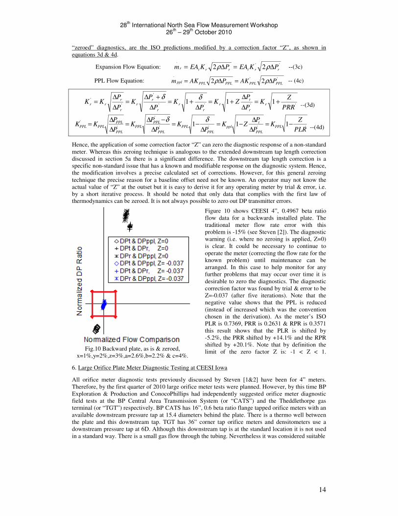
x=1%,y=2%,z=3%,a=2.6%,b=2.2% & c=4%.

Figure 10 shows CEESI 4”, 0.4967 beta ratio

flow data for a backwards installed plate. The

traditional meter flow rate error with this

problem is -15% (see Steven [2]). The diagnostic

warning (i.e. where no zeroing is applied, Z=0)

is clear. It could be necessary to continue to

operate the meter (correcting the flow rate for the

known problem) until maintenance can be

arranged. In this case to help monitor for any

further problems that may occur over time it is

desirable to zero the diagnostics. The diagnostic

correction factor was found by trial & error to be

Z=-0.037 (after five iterations). Note that the

negative value shows that the PPL is reduced

(instead of increased which was the convention

chosen in the derivation). As the meter’s ISO

PLR is 0.7369, PRR is 0.2631 & RPR is 0.3571

this result shows that the PLR is shifted by

-5.2%, the PRR shifted by +14.1% and the RPR

shifted by +20.1%. Note that by definition the

limit of the zero factor Z is: -1 < Z < 1.

6. Large Orifice Plate Meter Diagnostic Testing at CEESI Iowa

All orifice meter diagnostic tests previously discussed by Steven [1&2] have been for 4” meters.

Therefore, by the first quarter of 2010 large orifice meter tests were planned. However, by this time BP

Exploration & Production and ConocoPhillips had independently suggested orifice meter diagnostic

field tests at the BP Central Area Transmission System (or “CATS”) and the Theddlethorpe gas

terminal (or “TGT”) respectively. BP CATS has 16”, 0.6 beta ratio flange tapped orifice meters with an

available downstream pressure tap at 15.4 diameters behind the plate. There is a thermo well between

the plate and this downstream tap. TGT has 36” corner tap orifice meters and densitometers use a

downstream pressure tap at 6D. Although this downstream tap is at the standard location it is not used

in a standard way. There is a small gas flow through the tubing. Nevertheless it was considered suitable

28th International North Sea Flow Measurement Workshop

26th – 29

th October 2010

15

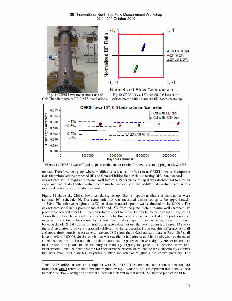
Fig.11 CEESI Iowa meter mock ups of Fig.12 CEESI Iowa 16”, sch 80, 0.6 beta ratio

CoP Theddlethorpe & BP CATS installations. orifice meter with a standard 6D downstream tap.

Figure 13 CEESI Iowa 16” paddle plate orifice meter results for downstream tapping at 6D & 15D.

for use. Therefore, test plans where modified to test a 16” orifice run at CEESI Iowa to incorporate

tests that mimicked the proposed BP and ConocoPhillips field trials. As testing BP’s non-standard1

downstream set up required a thermo well before a 15.4D pressure tap it was decided not to alter an

expensive 16” dual chamber orifice meter run but rather use a 16” paddle plate orifice meter with a

modified carbon steel downstream spool.

Figure 11 shows the CEESI Iowa test during set up. The 16” spools available at short notice were

nominal 16”, schedule 80. The actual inlet ID was measured during set up to be approximately

14.380”. The relative roughness (e/D) of these standard spools was estimated to be 0.0001. The

downstream spool had a pressure tap at 6D and 15D from the plate. Note a thermo well / temperature

probe was included after 6D in the downstream spool to mimic BP CATS meter installation. Figure 13

shows the ISO discharge coefficient predictions for this beta ratio across the tested Reynolds number

range and the actual values found by the test. Note that as required there is no significant difference

between the 6D & 15D test as the traditional meter does not use the downstream tap. Figure 13 shows

the ISO prediction to be very marginally different to the test results. However, this difference is small

and not entirely surprising for several reasons. ISO states that a 0.6 beta ratio plate at Re > 10e7 shall

have an e/D < 0.00006. So the spools that were available had almost double the allowed roughness of

an orifice meter run. Also note that by their nature paddle plates can have a slightly greater uncertainty

than orifice fittings due to the difficulty in manually aligning the plate to the precise centre line.

Furthermore it must be noted that the ISO performance criteria states that the 0.5% uncertainty assumes

that beta ratio, inlet diameter, Reynolds number and relative roughness are known precisely. The

1 BP CATS orifice meters are compliant with ISO 5167. The comment here about a non-standard

installation solely refers to the downstream pressure tap – which is not a component traditionally used

to meter the flow – being positioned at a location different to that which ISO uses to predict the PLR.

28th International North Sea Flow Measurement Workshop

26th – 29

th October 2010

16

reference Reynolds number is derived from the facility’s reference mass flow metering system with a

0.3% uncertainty. The DP’s read have the standard uncertainties of well maintained DP transmitters.

There is an uncertainty associated with the diameter and relative roughness measurement. Therefore, in

balance, for a large paddle plate with relatively rough spools these results looked reasonable.

Figure 12 shows the diagnostic results for the case of the downstream tap at 6D. The diagnostic

sensitivities are set at the values previously suggested by Steven [2], i.e. x=1%, y=2%, z=3%, a=2.6%,

b=2.2% & c=4%. Clearly the diagnostics show no problem for the standard case of a 6D downstream

tap. It can be seen that the points are not in fact at the origin but it should be understood that the origin

represents the precise ISO predictions with no uncertainty in either the ISO predictions or in any of the

experimental results. Hence, all orifice meters operating correctly shall have all diagnostic points inside

the NDB but these points will be scattered around the origin. In such cases no correction is necessary

(although zeroing can eradicate trends inside the NDB and tweak the system’s diagnostic sensitivity).

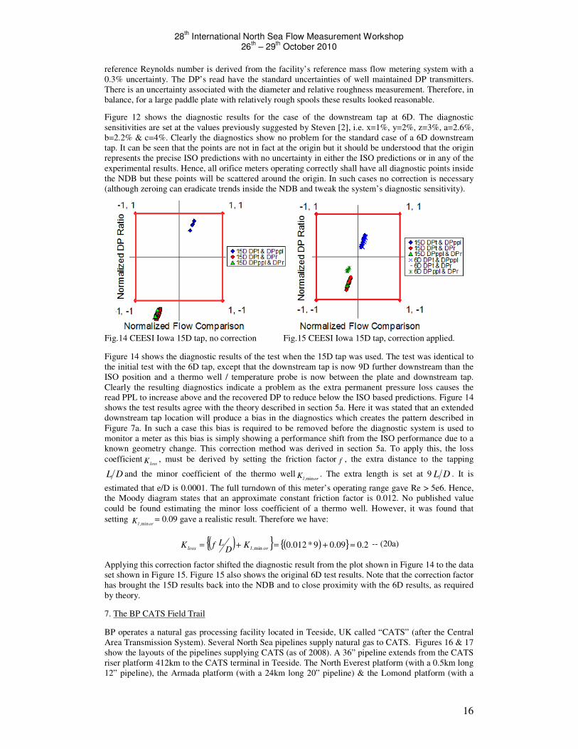
Fig.14 CEESI Iowa 15D tap, no correction Fig.15 CEESI Iowa 15D tap, correction applied.

Figure 14 shows the diagnostic results of the test when the 15D tap was used. The test was identical to

the initial test with the 6D tap, except that the downstream tap is now 9D further downstream than the

ISO position and a thermo well / temperature probe is now between the plate and downstream tap.

Clearly the resulting diagnostics indicate a problem as the extra permanent pressure loss causes the

read PPL to increase above and the recovered DP to reduce below the ISO based predictions. Figure 14

shows the test results agree with the theory described in section 5a. Here it was stated that an extended

downstream tap location will produce a bias in the diagnostics which creates the pattern described in

Figure 7a. In such a case this bias is required to be removed before the diagnostic system is used to

monitor a meter as this bias is simply showing a performance shift from the ISO performance due to a

known geometry change. This correction method was derived in section 5a. To apply this, the loss

coefficientlossK , must be derived by setting the friction factor f , the extra distance to the tapping

DL and the minor coefficient of the thermo wellorlK min,

. The extra length is set at 9 DL . It is

estimated that e/D is 0.0001. The full turndown of this meter’s operating range gave Re > 5e6. Hence,

the Moody diagram states that an approximate constant friction factor is 0.012. No published value

could be found estimating the minor loss coefficient of a thermo well. However, it was found that

setting orlK min,

= 0.09 gave a realistic result. Therefore we have:

( ){ } ( ){ } 2.009.09*012.0min, ≈+=+= orlloss KD

LfK -- (20a)

Applying this correction factor shifted the diagnostic result from the plot shown in Figure 14 to the data

set shown in Figure 15. Figure 15 also shows the original 6D test results. Note that the correction factor

has brought the 15D results back into the NDB and to close proximity with the 6D results, as required

by theory.

7. The BP CATS Field Trail

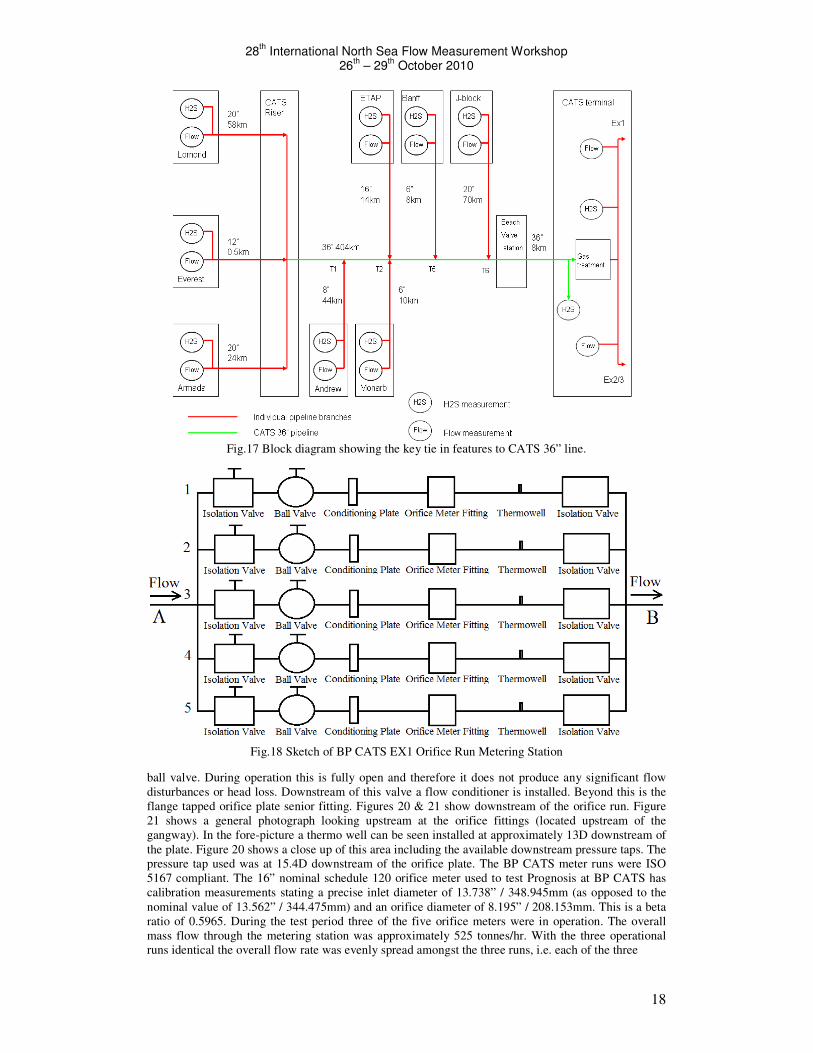
BP operates a natural gas processing facility located in Teeside, UK called “CATS” (after the Central

Area Transmission System). Several North Sea pipelines supply natural gas to CATS. Figures 16 & 17

show the layouts of the pipelines supplying CATS (as of 2008). A 36” pipeline extends from the CATS

riser platform 412km to the CATS terminal in Teeside. The North Everest platform (with a 0.5km long

12” pipeline), the Armada platform (with a 24km long 20” pipeline) & the Lomond platform (with a

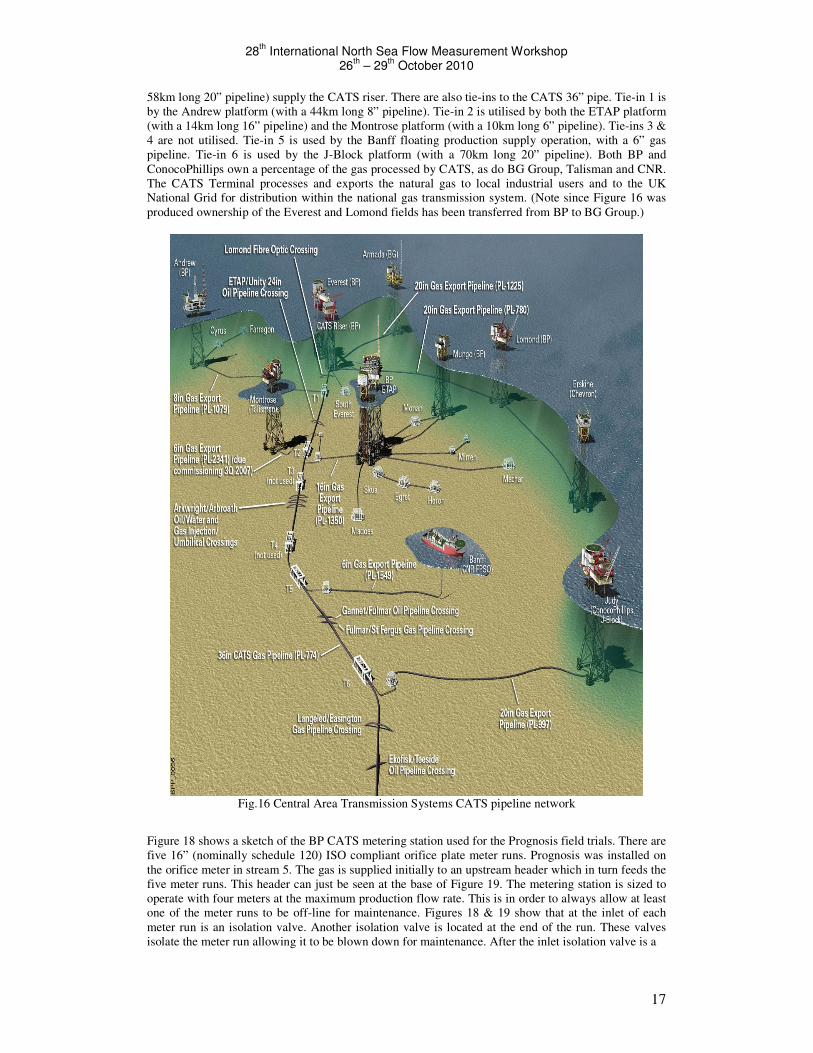
28th International North Sea Flow Measurement Workshop

26th – 29

th October 2010

17

58km long 20” pipeline) supply the CATS riser. There are also tie-ins to the CATS 36” pipe. Tie-in 1 is

by the Andrew platform (with a 44km long 8” pipeline). Tie-in 2 is utilised by both the ETAP platform

(with a 14km long 16” pipeline) and the Montrose platform (with a 10km long 6” pipeline). Tie-ins 3 &

4 are not utilised. Tie-in 5 is used by the Banff floating production supply operation, with a 6” gas

pipeline. Tie-in 6 is used by the J-Block platform (with a 70km long 20” pipeline). Both BP and

ConocoPhillips own a percentage of the gas processed by CATS, as do BG Group, Talisman and CNR.

The CATS Terminal processes and exports the natural gas to local industrial users and to the UK

National Grid for distribution within the national gas transmission system. (Note since Figure 16 was

produced ownership of the Everest and Lomond fields has been transferred from BP to BG Group.)

Fig.16 Central Area Transmission Systems CATS pipeline network

Figure 18 shows a sketch of the BP CATS metering station used for the Prognosis field trials. There are

five 16” (nominally schedule 120) ISO compliant orifice plate meter runs. Prognosis was installed on

the orifice meter in stream 5. The gas is supplied initially to an upstream header which in turn feeds the

five meter runs. This header can just be seen at the base of Figure 19. The metering station is sized to

operate with four meters at the maximum production flow rate. This is in order to always allow at least

one of the meter runs to be off-line for maintenance. Figures 18 & 19 show that at the inlet of each

meter run is an isolation valve. Another isolation valve is located at the end of the run. These valves

isolate the meter run allowing it to be blown down for maintenance. After the inlet isolation valve is a

28th International North Sea Flow Measurement Workshop

26th – 29

th October 2010

18

Fig.17 Block diagram showing the key tie in features to CATS 36” line.

Fig.18 Sketch of BP CATS EX1 Orifice Run Metering Station

ball valve. During operation this is fully open and therefore it does not produce any significant flow

disturbances or head loss. Downstream of this valve a flow conditioner is installed. Beyond this is the

flange tapped orifice plate senior fitting. Figures 20 & 21 show downstream of the orifice run. Figure

21 shows a general photograph looking upstream at the orifice fittings (located upstream of the

gangway). In the fore-picture a thermo well can be seen installed at approximately 13D downstream of

the plate. Figure 20 shows a close up of this area including the available downstream pressure taps. The

pressure tap used was at 15.4D downstream of the orifice plate. The BP CATS meter runs were ISO

5167 compliant. The 16” nominal schedule 120 orifice meter used to test Prognosis at BP CATS has

calibration measurements stating a precise inlet diameter of 13.738” / 348.945mm (as opposed to the

nominal value of 13.562” / 344.475mm) and an orifice diameter of 8.195” / 208.153mm. This is a beta

ratio of 0.5965. During the test period three of the five orifice meters were in operation. The overall

mass flow through the metering station was approximately 525 tonnes/hr. With the three operational

runs identical the overall flow rate was evenly spread amongst the three runs, i.e. each of the three

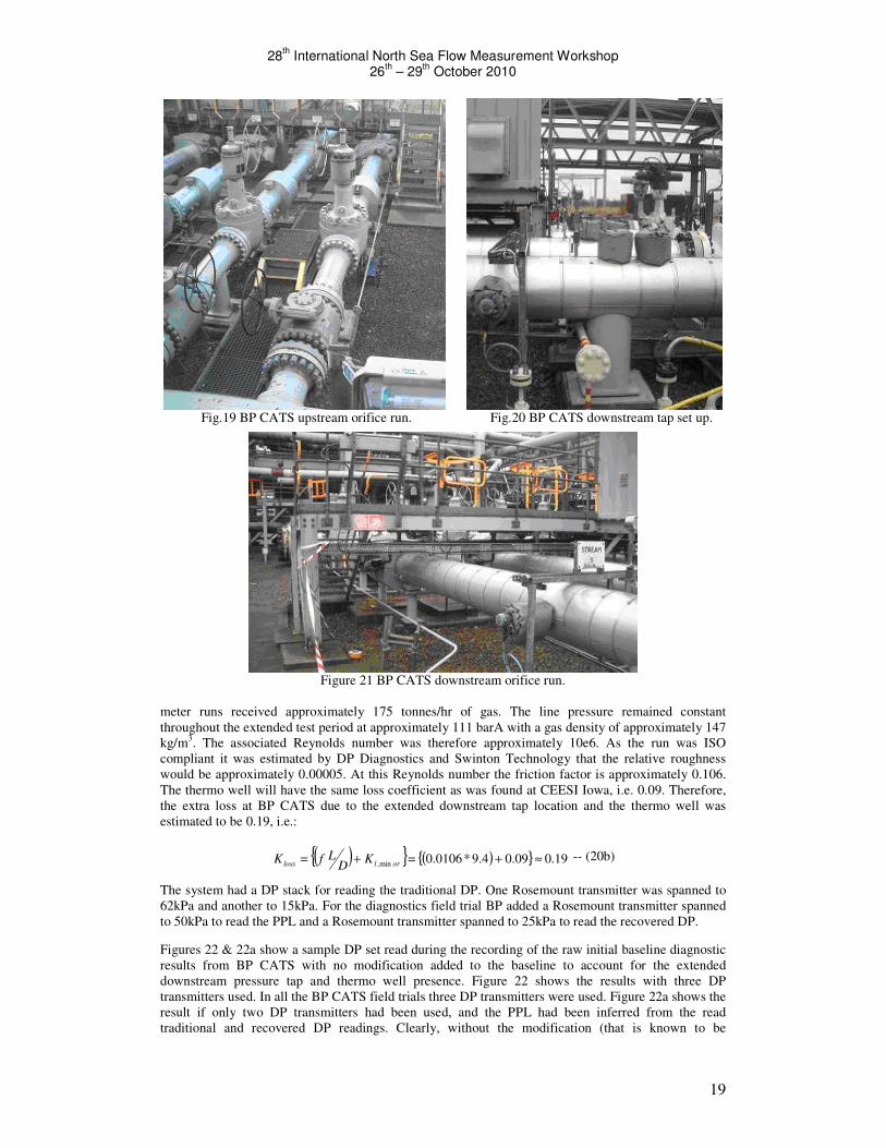
28th International North Sea Flow Measurement Workshop

26th – 29

th October 2010

19

Fig.19 BP CATS upstream orifice run. Fig.20 BP CATS downstream tap set up.

Figure 21 BP CATS downstream orifice run.

meter runs received approximately 175 tonnes/hr of gas. The line pressure remained constant

throughout the extended test period at approximately 111 barA with a gas density of approximately 147

kg/m3. The associated Reynolds number was therefore approximately 10e6. As the run was ISO

compliant it was estimated by DP Diagnostics and Swinton Technology that the relative roughness

would be approximately 0.00005. At this Reynolds number the friction factor is approximately 0.106.

The thermo well will have the same loss coefficient as was found at CEESI Iowa, i.e. 0.09. Therefore,

the extra loss at BP CATS due to the extended downstream tap location and the thermo well was

estimated to be 0.19, i.e.:

( ){ } ( ){ } 19.009.04.9*0106.0min, ≈+=+= orlloss KD

LfK -- (20b)

The system had a DP stack for reading the traditional DP. One Rosemount transmitter was spanned to

62kPa and another to 15kPa. For the diagnostics field trial BP added a Rosemount transmitter spanned

to 50kPa to read the PPL and a Rosemount transmitter spanned to 25kPa to read the recovered DP.

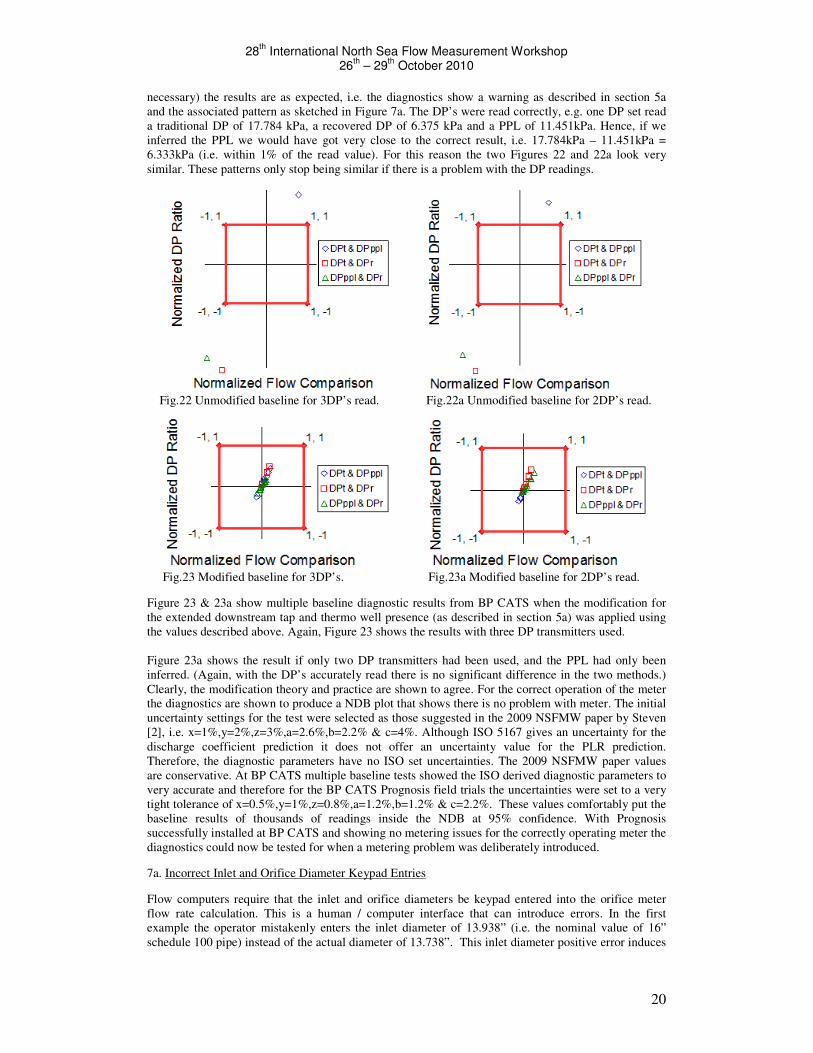
Figures 22 & 22a show a sample DP set read during the recording of the raw initial baseline diagnostic

results from BP CATS with no modification added to the baseline to account for the extended

downstream pressure tap and thermo well presence. Figure 22 shows the results with three DP

transmitters used. In all the BP CATS field trials three DP transmitters were used. Figure 22a shows the

result if only two DP transmitters had been used, and the PPL had been inferred from the read

traditional and recovered DP readings. Clearly, without the modification (that is known to be

28th International North Sea Flow Measurement Workshop

26th – 29

th October 2010

20

necessary) the results are as expected, i.e. the diagnostics show a warning as described in section 5a

and the associated pattern as sketched in Figure 7a. The DP’s were read correctly, e.g. one DP set read

a traditional DP of 17.784 kPa, a recovered DP of 6.375 kPa and a PPL of 11.451kPa. Hence, if we

inferred the PPL we would have got very close to the correct result, i.e. 17.784kPa – 11.451kPa =

6.333kPa (i.e. within 1% of the read value). For this reason the two Figures 22 and 22a look very

similar. These patterns only stop being similar if there is a problem with the DP readings.

Fig.22 Unmodified baseline for 3DP’s read. Fig.22a Unmodified baseline for 2DP’s read.

Fig.23 Modified baseline for 3DP’s. Fig.23a Modified baseline for 2DP’s read.

Figure 23 & 23a show multiple baseline diagnostic results from BP CATS when the modification for

the extended downstream tap and thermo well presence (as described in section 5a) was applied using

the values described above. Again, Figure 23 shows the results with three DP transmitters used.

Figure 23a shows the result if only two DP transmitters had been used, and the PPL had only been

inferred. (Again, with the DP’s accurately read there is no significant difference in the two methods.)

Clearly, the modification theory and practice are shown to agree. For the correct operation of the meter

the diagnostics are shown to produce a NDB plot that shows there is no problem with meter. The initial

uncertainty settings for the test were selected as those suggested in the 2009 NSFMW paper by Steven

[2], i.e. x=1%,y=2%,z=3%,a=2.6%,b=2.2% & c=4%. Although ISO 5167 gives an uncertainty for the

discharge coefficient prediction it does not offer an uncertainty value for the PLR prediction.

Therefore, the diagnostic parameters have no ISO set uncertainties. The 2009 NSFMW paper values

are conservative. At BP CATS multiple baseline tests showed the ISO derived diagnostic parameters to

very accurate and therefore for the BP CATS Prognosis field trials the uncertainties were set to a very

tight tolerance of x=0.5%,y=1%,z=0.8%,a=1.2%,b=1.2% & c=2.2%. These values comfortably put the

baseline results of thousands of readings inside the NDB at 95% confidence. With Prognosis

successfully installed at BP CATS and showing no metering issues for the correctly operating meter the

diagnostics could now be tested for when a metering problem was deliberately introduced.

7a. Incorrect Inlet and Orifice Diameter Keypad Entries

Flow computers require that the inlet and orifice diameters be keypad entered into the orifice meter

flow rate calculation. This is a human / computer interface that can introduce errors. In the first

example the operator mistakenly enters the inlet diameter of 13.938” (i.e. the nominal value of 16”

schedule 100 pipe) instead of the actual diameter of 13.738”. This inlet diameter positive error induces

28th International North Sea Flow Measurement Workshop

26th – 29

th October 2010

21

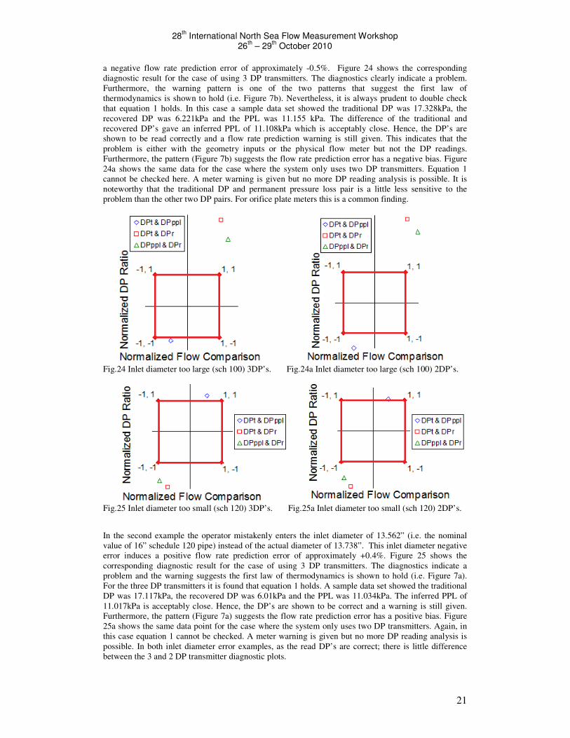
a negative flow rate prediction error of approximately -0.5%. Figure 24 shows the corresponding

diagnostic result for the case of using 3 DP transmitters. The diagnostics clearly indicate a problem.

Furthermore, the warning pattern is one of the two patterns that suggest the first law of

thermodynamics is shown to hold (i.e. Figure 7b). Nevertheless, it is always prudent to double check

that equation 1 holds. In this case a sample data set showed the traditional DP was 17.328kPa, the

recovered DP was 6.221kPa and the PPL was 11.155 kPa. The difference of the traditional and

recovered DP’s gave an inferred PPL of 11.108kPa which is acceptably close. Hence, the DP’s are

shown to be read correctly and a flow rate prediction warning is still given. This indicates that the

problem is either with the geometry inputs or the physical flow meter but not the DP readings.

Furthermore, the pattern (Figure 7b) suggests the flow rate prediction error has a negative bias. Figure

24a shows the same data for the case where the system only uses two DP transmitters. Equation 1

cannot be checked here. A meter warning is given but no more DP reading analysis is possible. It is

noteworthy that the traditional DP and permanent pressure loss pair is a little less sensitive to the

problem than the other two DP pairs. For orifice plate meters this is a common finding.

Fig.24 Inlet diameter too large (sch 100) 3DP’s. Fig.24a Inlet diameter too large (sch 100) 2DP’s.

Fig.25 Inlet diameter too small (sch 120) 3DP’s. Fig.25a Inlet diameter too small (sch 120) 2DP’s.

In the second example the operator mistakenly enters the inlet diameter of 13.562” (i.e. the nominal

value of 16” schedule 120 pipe) instead of the actual diameter of 13.738”. This inlet diameter negative

error induces a positive flow rate prediction error of approximately +0.4%. Figure 25 shows the

corresponding diagnostic result for the case of using 3 DP transmitters. The diagnostics indicate a

problem and the warning suggests the first law of thermodynamics is shown to hold (i.e. Figure 7a).

For the three DP transmitters it is found that equation 1 holds. A sample data set showed the traditional

DP was 17.117kPa, the recovered DP was 6.01kPa and the PPL was 11.034kPa. The inferred PPL of

11.017kPa is acceptably close. Hence, the DP’s are shown to be correct and a warning is still given.

Furthermore, the pattern (Figure 7a) suggests the flow rate prediction error has a positive bias. Figure

25a shows the same data point for the case where the system only uses two DP transmitters. Again, in

this case equation 1 cannot be checked. A meter warning is given but no more DP reading analysis is

possible. In both inlet diameter error examples, as the read DP’s are correct; there is little difference

between the 3 and 2 DP transmitter diagnostic plots.

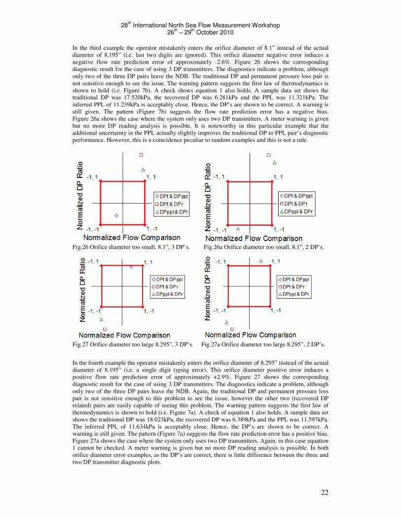
28th International North Sea Flow Measurement Workshop

26th – 29

th October 2010

22

In the third example the operator mistakenly enters the orifice diameter of 8.1” instead of the actual

diameter of 8.195” (i.e. last two digits are ignored). This orifice diameter negative error induces a

negative flow rate prediction error of approximately -2.6%. Figure 26 shows the corresponding

diagnostic result for the case of using 3 DP transmitters. The diagnostics indicate a problem, although

only two of the three DP pairs leave the NDB. The traditional DP and permanent pressure loss pair is

not sensitive enough to see the issue. The warning pattern suggests the first law of thermodynamics is

shown to hold (i.e. Figure 7b). A check shows equation 1 also holds. A sample data set shows the

traditional DP was 17.520kPa, the recovered DP was 6.281kPa and the PPL was 11.321kPa. The

inferred PPL of 11.239kPa is acceptably close. Hence, the DP’s are shown to be correct. A warning is

still given. The pattern (Figure 7b) suggests the flow rate prediction error has a negative bias.

Figure 26a shows the case where the system only uses two DP transmitters. A meter warning is given

but no more DP reading analysis is possible. It is noteworthy in this particular example that the

additional uncertainty in the PPL actually slightly improves the traditional DP to PPL pair’s diagnostic

performance. However, this is a coincidence peculiar to random examples and this is not a rule.

Fig.26 Orifice diameter too small, 8.1”, 3 DP’s. Fig.26a Orifice diameter too small, 8.1”, 2 DP’s.

Fig.27 Orifice diameter too large 8.295”, 3 DP’s. Fig.27a Orifice diameter too large 8.295”, 2 DP’s.

In the fourth example the operator mistakenly enters the orifice diameter of 8.295” instead of the actual

diameter of 8.195” (i.e. a single digit typing error). This orifice diameter positive error induces a

positive flow rate prediction error of approximately +2.9%. Figure 27 shows the corresponding

diagnostic result for the case of using 3 DP transmitters. The diagnostics indicate a problem, although

only two of the three DP pairs leave the NDB. Again, the traditional DP and permanent pressure loss

pair is not sensitive enough to this problem to see the issue, however the other two (recovered DP

related) pairs are easily capable of seeing this problem. The warning pattern suggests the first law of

thermodynamics is shown to hold (i.e. Figure 7a). A check of equation 1 also holds. A sample data set

shows the traditional DP was 18.023kPa, the recovered DP was 6.389kPa and the PPL was 11.597kPa.

The inferred PPL of 11.634kPa is acceptably close. Hence, the DP’s are shown to be correct. A

warning is still given. The pattern (Figure 7a) suggests the flow rate prediction error has a positive bias.

Figure 27a shows the case where the system only uses two DP transmitters. Again, in this case equation

1 cannot be checked. A meter warning is given but no more DP reading analysis is possible. In both

orifice diameter error examples, as the DP’s are correct, there is little difference between the three and

two DP transmitter diagnostic plots.

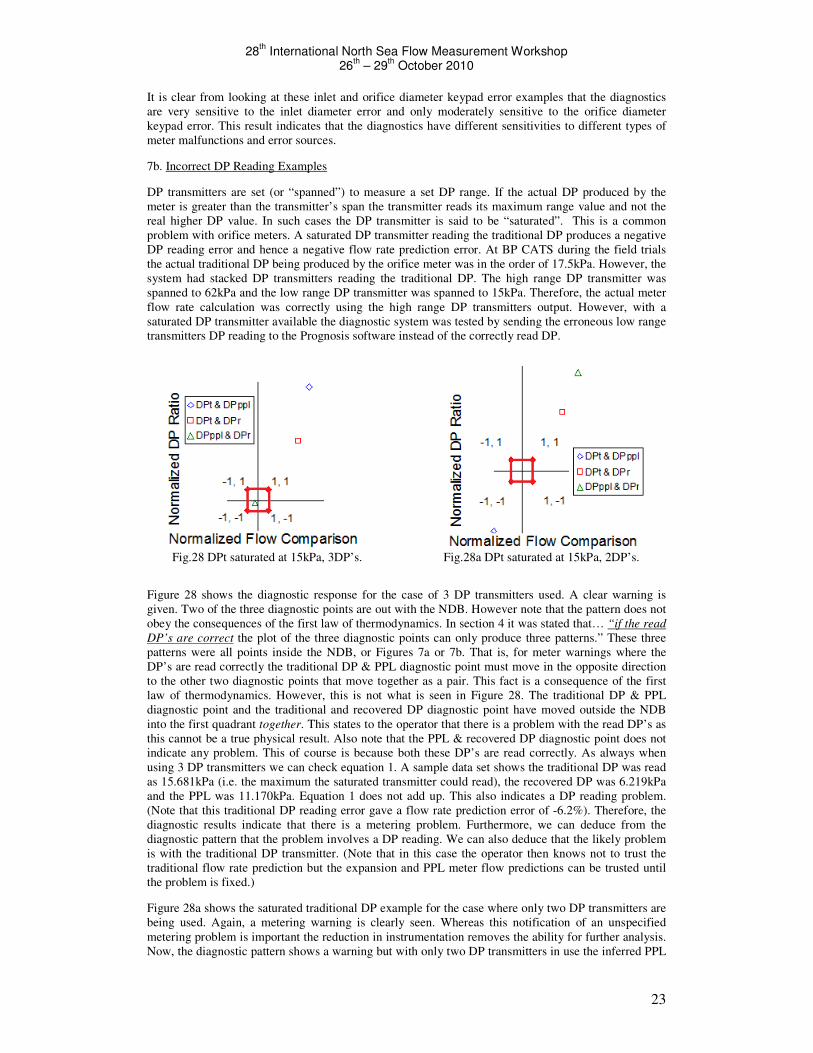
28th International North Sea Flow Measurement Workshop

26th – 29

th October 2010

23

It is clear from looking at these inlet and orifice diameter keypad error examples that the diagnostics

are very sensitive to the inlet diameter error and only moderately sensitive to the orifice diameter

keypad error. This result indicates that the diagnostics have different sensitivities to different types of

meter malfunctions and error sources.

7b. Incorrect DP Reading Examples

DP transmitters are set (or “spanned”) to measure a set DP range. If the actual DP produced by the

meter is greater than the transmitter’s span the transmitter reads its maximum range value and not the

real higher DP value. In such cases the DP transmitter is said to be “saturated”. This is a common

problem with orifice meters. A saturated DP transmitter reading the traditional DP produces a negative

DP reading error and hence a negative flow rate prediction error. At BP CATS during the field trials

the actual traditional DP being produced by the orifice meter was in the order of 17.5kPa. However, the

system had stacked DP transmitters reading the traditional DP. The high range DP transmitter was

spanned to 62kPa and the low range DP transmitter was spanned to 15kPa. Therefore, the actual meter

flow rate calculation was correctly using the high range DP transmitters output. However, with a

saturated DP transmitter available the diagnostic system was tested by sending the erroneous low range

transmitters DP reading to the Prognosis software instead of the correctly read DP.

Fig.28 DPt saturated at 15kPa, 3DP’s. Fig.28a DPt saturated at 15kPa, 2DP’s.

Figure 28 shows the diagnostic response for the case of 3 DP transmitters used. A clear warning is

given. Two of the three diagnostic points are out with the NDB. However note that the pattern does not

obey the consequences of the first law of thermodynamics. In section 4 it was stated that… “if the read

DP’s are correct the plot of the three diagnostic points can only produce three patterns.” These three

patterns were all points inside the NDB, or Figures 7a or 7b. That is, for meter warnings where the

DP’s are read correctly the traditional DP & PPL diagnostic point must move in the opposite direction

to the other two diagnostic points that move together as a pair. This fact is a consequence of the first

law of thermodynamics. However, this is not what is seen in Figure 28. The traditional DP & PPL

diagnostic point and the traditional and recovered DP diagnostic point have moved outside the NDB

into the first quadrant together. This states to the operator that there is a problem with the read DP’s as

this cannot be a true physical result. Also note that the PPL & recovered DP diagnostic point does not

indicate any problem. This of course is because both these DP’s are read correctly. As always when

using 3 DP transmitters we can check equation 1. A sample data set shows the traditional DP was read

as 15.681kPa (i.e. the maximum the saturated transmitter could read), the recovered DP was 6.219kPa

and the PPL was 11.170kPa. Equation 1 does not add up. This also indicates a DP reading problem.

(Note that this traditional DP reading error gave a flow rate prediction error of -6.2%). Therefore, the

diagnostic results indicate that there is a metering problem. Furthermore, we can deduce from the

diagnostic pattern that the problem involves a DP reading. We can also deduce that the likely problem

is with the traditional DP transmitter. (Note that in this case the operator then knows not to trust the

traditional flow rate prediction but the expansion and PPL meter flow predictions can be trusted until

the problem is fixed.)

Figure 28a shows the saturated traditional DP example for the case where only two DP transmitters are

being used. Again, a metering warning is clearly seen. Whereas this notification of an unspecified

metering problem is important the reduction in instrumentation removes the ability for further analysis.

Now, the diagnostic pattern shows a warning but with only two DP transmitters in use the inferred PPL

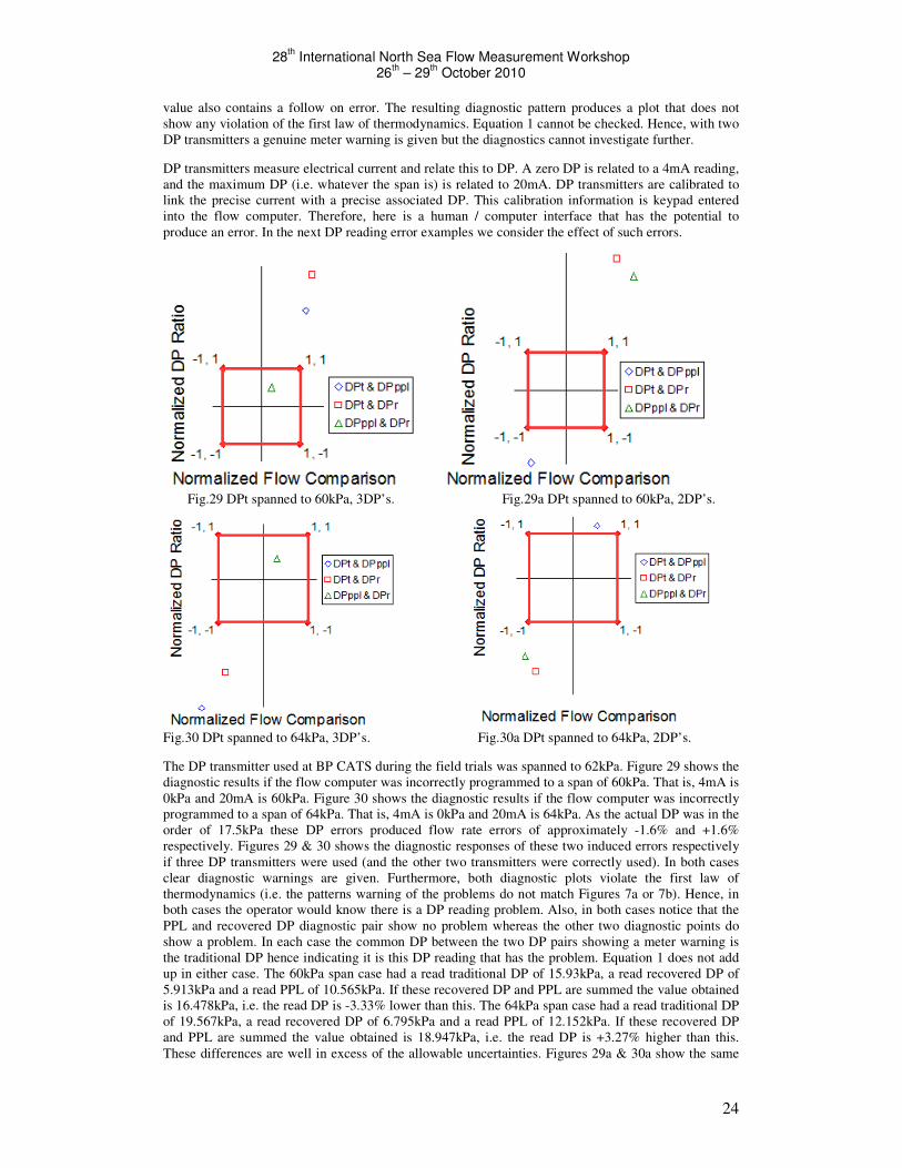
28th International North Sea Flow Measurement Workshop

26th – 29

th October 2010

24

value also contains a follow on error. The resulting diagnostic pattern produces a plot that does not

show any violation of the first law of thermodynamics. Equation 1 cannot be checked. Hence, with two

DP transmitters a genuine meter warning is given but the diagnostics cannot investigate further.

DP transmitters measure electrical current and relate this to DP. A zero DP is related to a 4mA reading,

and the maximum DP (i.e. whatever the span is) is related to 20mA. DP transmitters are calibrated to

link the precise current with a precise associated DP. This calibration information is keypad entered

into the flow computer. Therefore, here is a human / computer interface that has the potential to

produce an error. In the next DP reading error examples we consider the effect of such errors.

Fig.29 DPt spanned to 60kPa, 3DP’s. Fig.29a DPt spanned to 60kPa, 2DP’s.

Fig.30 DPt spanned to 64kPa, 3DP’s. Fig.30a DPt spanned to 64kPa, 2DP’s.

The DP transmitter used at BP CATS during the field trials was spanned to 62kPa. Figure 29 shows the

diagnostic results if the flow computer was incorrectly programmed to a span of 60kPa. That is, 4mA is

0kPa and 20mA is 60kPa. Figure 30 shows the diagnostic results if the flow computer was incorrectly

programmed to a span of 64kPa. That is, 4mA is 0kPa and 20mA is 64kPa. As the actual DP was in the

order of 17.5kPa these DP errors produced flow rate errors of approximately -1.6% and +1.6%

respectively. Figures 29 & 30 shows the diagnostic responses of these two induced errors respectively

if three DP transmitters were used (and the other two transmitters were correctly used). In both cases

clear diagnostic warnings are given. Furthermore, both diagnostic plots violate the first law of

thermodynamics (i.e. the patterns warning of the problems do not match Figures 7a or 7b). Hence, in

both cases the operator would know there is a DP reading problem. Also, in both cases notice that the

PPL and recovered DP diagnostic pair show no problem whereas the other two diagnostic points do

show a problem. In each case the common DP between the two DP pairs showing a meter warning is

the traditional DP hence indicating it is this DP reading that has the problem. Equation 1 does not add

up in either case. The 60kPa span case had a read traditional DP of 15.93kPa, a read recovered DP of

5.913kPa and a read PPL of 10.565kPa. If these recovered DP and PPL are summed the value obtained

is 16.478kPa, i.e. the read DP is -3.33% lower than this. The 64kPa span case had a read traditional DP

of 19.567kPa, a read recovered DP of 6.795kPa and a read PPL of 12.152kPa. If these recovered DP

and PPL are summed the value obtained is 18.947kPa, i.e. the read DP is +3.27% higher than this.

These differences are well in excess of the allowable uncertainties. Figures 29a & 30a show the same

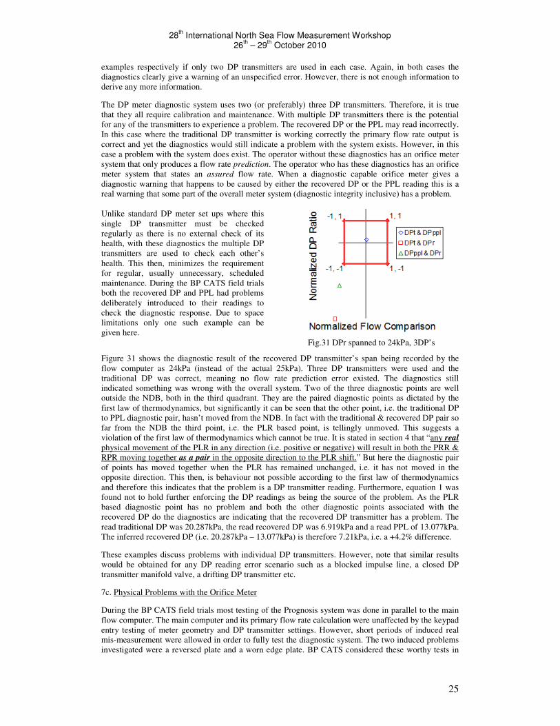
28th International North Sea Flow Measurement Workshop

26th – 29

th October 2010

25

examples respectively if only two DP transmitters are used in each case. Again, in both cases the

diagnostics clearly give a warning of an unspecified error. However, there is not enough information to

derive any more information.

The DP meter diagnostic system uses two (or preferably) three DP transmitters. Therefore, it is true

that they all require calibration and maintenance. With multiple DP transmitters there is the potential

for any of the transmitters to experience a problem. The recovered DP or the PPL may read incorrectly.

In this case where the traditional DP transmitter is working correctly the primary flow rate output is

correct and yet the diagnostics would still indicate a problem with the system exists. However, in this

case a problem with the system does exist. The operator without these diagnostics has an orifice meter

system that only produces a flow rate prediction. The operator who has these diagnostics has an orifice

meter system that states an assured flow rate. When a diagnostic capable orifice meter gives a

diagnostic warning that happens to be caused by either the recovered DP or the PPL reading this is a

real warning that some part of the overall meter system (diagnostic integrity inclusive) has a problem.

Unlike standard DP meter set ups where this

single DP transmitter must be checked

regularly as there is no external check of its

health, with these diagnostics the multiple DP

transmitters are used to check each other’s

health. This then, minimizes the requirement

for regular, usually unnecessary, scheduled

maintenance. During the BP CATS field trials

both the recovered DP and PPL had problems

deliberately introduced to their readings to

check the diagnostic response. Due to space

limitations only one such example can be

given here.

Fig.31 DPr spanned to 24kPa, 3DP’s

Figure 31 shows the diagnostic result of the recovered DP transmitter’s span being recorded by the

flow computer as 24kPa (instead of the actual 25kPa). Three DP transmitters were used and the

traditional DP was correct, meaning no flow rate prediction error existed. The diagnostics still

indicated something was wrong with the overall system. Two of the three diagnostic points are well

outside the NDB, both in the third quadrant. They are the paired diagnostic points as dictated by the

first law of thermodynamics, but significantly it can be seen that the other point, i.e. the traditional DP

to PPL diagnostic pair, hasn’t moved from the NDB. In fact with the traditional & recovered DP pair so

far from the NDB the third point, i.e. the PLR based point, is tellingly unmoved. This suggests a

violation of the first law of thermodynamics which cannot be true. It is stated in section 4 that “any real

physical movement of the PLR in any direction (i.e. positive or negative) will result in both the PRR &

RPR moving together as a pair in the opposite direction to the PLR shift.” But here the diagnostic pair

of points has moved together when the PLR has remained unchanged, i.e. it has not moved in the

opposite direction. This then, is behaviour not possible according to the first law of thermodynamics

and therefore this indicates that the problem is a DP transmitter reading. Furthermore, equation 1 was

found not to hold further enforcing the DP readings as being the source of the problem. As the PLR

based diagnostic point has no problem and both the other diagnostic points associated with the

recovered DP do the diagnostics are indicating that the recovered DP transmitter has a problem. The

read traditional DP was 20.287kPa, the read recovered DP was 6.919kPa and a read PPL of 13.077kPa.

The inferred recovered DP (i.e. 20.287kPa – 13.077kPa) is therefore 7.21kPa, i.e. a +4.2% difference.

These examples discuss problems with individual DP transmitters. However, note that similar results

would be obtained for any DP reading error scenario such as a blocked impulse line, a closed DP

transmitter manifold valve, a drifting DP transmitter etc.

7c. Physical Problems with the Orifice Meter

During the BP CATS field trials most testing of the Prognosis system was done in parallel to the main

flow computer. The main computer and its primary flow rate calculation were unaffected by the keypad

entry testing of meter geometry and DP transmitter settings. However, short periods of induced real

mis-measurement were allowed in order to fully test the diagnostic system. The two induced problems

investigated were a reversed plate and a worn edge plate. BP CATS considered these worthy tests in

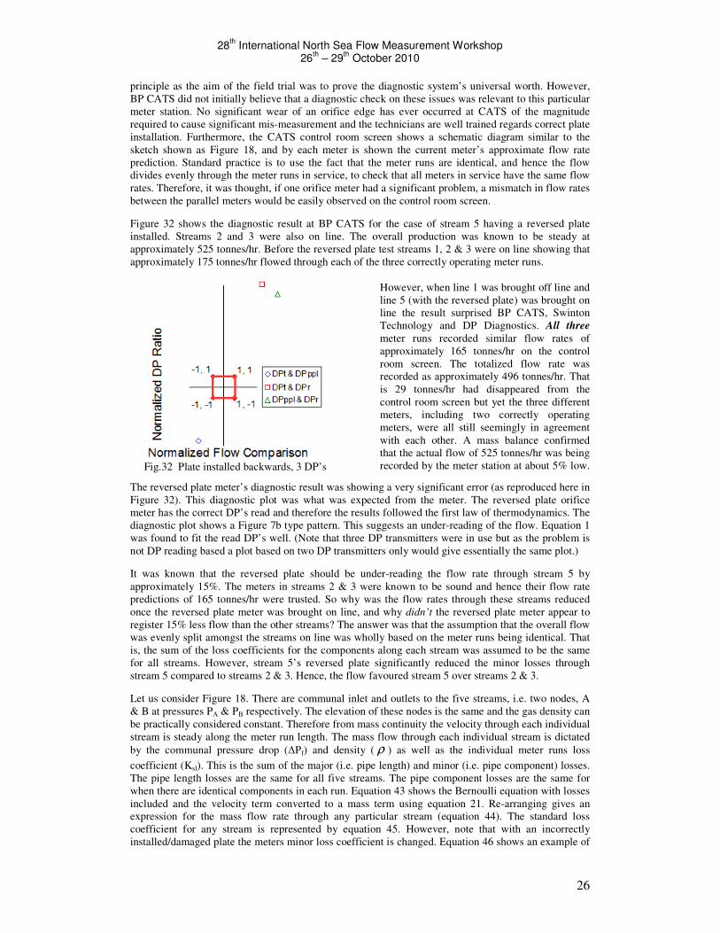
28th International North Sea Flow Measurement Workshop

26th – 29

th October 2010

26

principle as the aim of the field trial was to prove the diagnostic system’s universal worth. However,

BP CATS did not initially believe that a diagnostic check on these issues was relevant to this particular

meter station. No significant wear of an orifice edge has ever occurred at CATS of the magnitude

required to cause significant mis-measurement and the technicians are well trained regards correct plate

installation. Furthermore, the CATS control room screen shows a schematic diagram similar to the

sketch shown as Figure 18, and by each meter is shown the current meter’s approximate flow rate

prediction. Standard practice is to use the fact that the meter runs are identical, and hence the flow

divides evenly through the meter runs in service, to check that all meters in service have the same flow

rates. Therefore, it was thought, if one orifice meter had a significant problem, a mismatch in flow rates

between the parallel meters would be easily observed on the control room screen.

Figure 32 shows the diagnostic result at BP CATS for the case of stream 5 having a reversed plate

installed. Streams 2 and 3 were also on line. The overall production was known to be steady at

approximately 525 tonnes/hr. Before the reversed plate test streams 1, 2 & 3 were on line showing that

approximately 175 tonnes/hr flowed through each of the three correctly operating meter runs.

Fig.32 Plate installed backwards, 3 DP’s

However, when line 1 was brought off line and

line 5 (with the reversed plate) was brought on

line the result surprised BP CATS, Swinton

Technology and DP Diagnostics. All three

meter runs recorded similar flow rates of

approximately 165 tonnes/hr on the control

room screen. The totalized flow rate was

recorded as approximately 496 tonnes/hr. That

is 29 tonnes/hr had disappeared from the

control room screen but yet the three different

meters, including two correctly operating

meters, were all still seemingly in agreement

with each other. A mass balance confirmed

that the actual flow of 525 tonnes/hr was being

recorded by the meter station at about 5% low.

The reversed plate meter’s diagnostic result was showing a very significant error (as reproduced here in

Figure 32). This diagnostic plot was what was expected from the meter. The reversed plate orifice

meter has the correct DP’s read and therefore the results followed the first law of thermodynamics. The

diagnostic plot shows a Figure 7b type pattern. This suggests an under-reading of the flow. Equation 1

was found to fit the read DP’s well. (Note that three DP transmitters were in use but as the problem is

not DP reading based a plot based on two DP transmitters only would give essentially the same plot.)

It was known that the reversed plate should be under-reading the flow rate through stream 5 by

approximately 15%. The meters in streams 2 & 3 were known to be sound and hence their flow rate

predictions of 165 tonnes/hr were trusted. So why was the flow rates through these streams reduced

once the reversed plate meter was brought on line, and why didn’t the reversed plate meter appear to

register 15% less flow than the other streams? The answer was that the assumption that the overall flow

was evenly split amongst the streams on line was wholly based on the meter runs being identical. That

is, the sum of the loss coefficients for the components along each stream was assumed to be the same

for all streams. However, stream 5’s reversed plate significantly reduced the minor losses through

stream 5 compared to streams 2 & 3. Hence, the flow favoured stream 5 over streams 2 & 3.

Let us consider Figure 18. There are communal inlet and outlets to the five streams, i.e. two nodes, A

& B at pressures PA & PB respectively. The elevation of these nodes is the same and the gas density can

be practically considered constant. Therefore from mass continuity the velocity through each individual

stream is steady along the meter run length. The mass flow through each individual stream is dictated

by the communal pressure drop (∆Pf) and density ( ρ ) as well as the individual meter runs loss

coefficient (Ksl). This is the sum of the major (i.e. pipe length) and minor (i.e. pipe component) losses.

The pipe length losses are the same for all five streams. The pipe component losses are the same for

when there are identical components in each run. Equation 43 shows the Bernoulli equation with losses

included and the velocity term converted to a mass term using equation 21. Re-arranging gives an

expression for the mass flow rate through any particular stream (equation 44). The standard loss

coefficient for any stream is represented by equation 45. However, note that with an incorrectly

installed/damaged plate the meters minor loss coefficient is changed. Equation 46 shows an example of

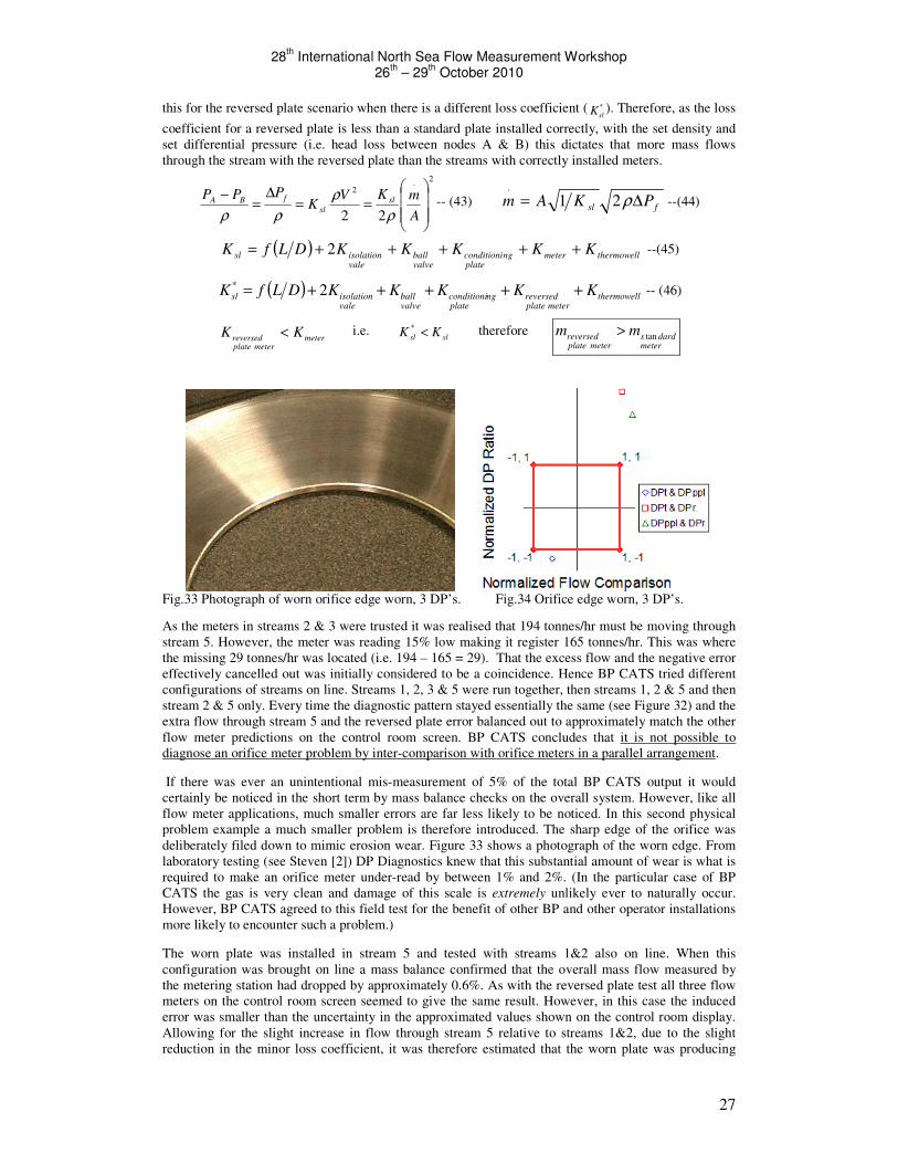
28th International North Sea Flow Measurement Workshop

26th – 29

th October 2010

27

this for the reversed plate scenario when there is a different loss coefficient ( *

slK ). Therefore, as the loss

coefficient for a reversed plate is less than a standard plate installed correctly, with the set density and

set differential pressure (i.e. head loss between nodes A & B) this dictates that more mass flows

through the stream with the reversed plate than the streams with correctly installed meters.

2.

2

22

==

∆=

−

A

mKVK

PPP sl

sl

fBA

ρ

ρ

ρρ-- (43)

fsl PKAm ∆= ρ21.

--(44)

( ) thermowellmeterplate

ngconditionivalveball

valeisolationsl KKKKKDLfK +++++= 2 --(45)

( ) thermowellmeterplate

reversedplate

ngconditionivalveball

valeisolationsl KKKKKDLfK +++++= 2*

-- (46)

metermeterplate

reversedKK < i.e.

slsl KK <* therefore meter

dardsmeterplate

reversed mm tan>

Fig.33 Photograph of worn orifice edge worn, 3 DP’s. Fig.34 Orifice edge worn, 3 DP’s.

As the meters in streams 2 & 3 were trusted it was realised that 194 tonnes/hr must be moving through

stream 5. However, the meter was reading 15% low making it register 165 tonnes/hr. This was where

the missing 29 tonnes/hr was located (i.e. 194 – 165 = 29). That the excess flow and the negative error

effectively cancelled out was initially considered to be a coincidence. Hence BP CATS tried different

configurations of streams on line. Streams 1, 2, 3 & 5 were run together, then streams 1, 2 & 5 and then

stream 2 & 5 only. Every time the diagnostic pattern stayed essentially the same (see Figure 32) and the

extra flow through stream 5 and the reversed plate error balanced out to approximately match the other

flow meter predictions on the control room screen. BP CATS concludes that it is not possible to

diagnose an orifice meter problem by inter-comparison with orifice meters in a parallel arrangement.

If there was ever an unintentional mis-measurement of 5% of the total BP CATS output it would

certainly be noticed in the short term by mass balance checks on the overall system. However, like all

flow meter applications, much smaller errors are far less likely to be noticed. In this second physical

problem example a much smaller problem is therefore introduced. The sharp edge of the orifice was

deliberately filed down to mimic erosion wear. Figure 33 shows a photograph of the worn edge. From

laboratory testing (see Steven [2]) DP Diagnostics knew that this substantial amount of wear is what is

required to make an orifice meter under-read by between 1% and 2%. (In the particular case of BP

CATS the gas is very clean and damage of this scale is extremely unlikely ever to naturally occur.

However, BP CATS agreed to this field test for the benefit of other BP and other operator installations

more likely to encounter such a problem.)

The worn plate was installed in stream 5 and tested with streams 1&2 also on line. When this

configuration was brought on line a mass balance confirmed that the overall mass flow measured by

the metering station had dropped by approximately 0.6%. As with the reversed plate test all three flow

meters on the control room screen seemed to give the same result. However, in this case the induced

error was smaller than the uncertainty in the approximated values shown on the control room display.

Allowing for the slight increase in flow through stream 5 relative to streams 1&2, due to the slight

reduction in the minor loss coefficient, it was therefore estimated that the worn plate was producing

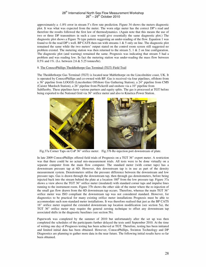
28th International North Sea Flow Measurement Workshop

26th – 29

th October 2010

28

approximately a -1.8% error in stream 5’s flow rate prediction. Figure 34 shows the meters diagnostic

plot. It was what was expected from the meter. The worn edge meter has the correct DP’s read and

therefore the results followed the first law of thermodynamics. (Again note that this means the use of

two or three DP transmitters in such a case would give essentially the same diagnostic plot.) The

diagnostic plot shows a Figure 7b type pattern suggesting an under-reading of the flow. Equation 1 was

found to fit the read DP’s well. BP CATS then ran with streams 1 & 5 only on line. The diagnostic plot

remained the same while the two meters’ output stated on the control room screen still suggested no

problem existed. The metering station was then returned to the stream 5, 1 & 2 on line configuration.

The diagnostic plot (and warning) remained the same. Prognosis was indicating that stream 5 had a

problem and was reading low. In fact the metering station was under-reading the mass flow between

0.5% and 1%. (I.e. between 2.6 & 5.25 tonnes/hr).

8. The ConocoPhillips Theddlethorpe Gas Terminal (TGT) Field Trail

The Theddlethorpe Gas Terminal (TGT) is located near Mablethorpe on the Lincolnshire coast, UK. It

is operated by ConocoPhillips and co-owned with BP. Gas is received via four pipelines, offshore from

a 36" pipeline from LOGGS (Lincolnshire Offshore Gas Gathering Station), a 24" pipeline from CMS

(Caister Murdoch Station), a 26" pipeline from Pickerill and onshore via a 10" pipeline from

Saltfleetby. These pipelines have various partners and equity splits. The gas is processed at TGT before

being exported to the National Grid via 36" orifice meter and also to Kinetica Power Station.

Fig.37a Corner Taps on CoP 36” orifice meter. Fig.37b Re-injection port downstream of plate.

In late 2009 ConocoPhillips offered field trials of Prognosis on a TGT 36” export meter. A restriction

was that there could be no actual mis-measurement trials. All tests were to be done virtually on a

separate computer from the main flow computer. The standard meter (with corner taps) has a

downstream pressure tap at 6D. However, this downstream tap is in use as part of the density

measurement system. Densitometers utilise the pressure difference between the downstream and low

pressure taps. Gas is drawn through the downstream tap, then through gas densitometers, before being

injected back into the stream behind the plate at a location 1800 from the low pressure tap. Figure 37a

shows a view above the TGT 36” orifice meter (insulated) with standard corner taps and impulse lines

running to the instrument room. Figure 37b shows the other side of the meter where the re-injection of

the small gas flow drawn from the 6D downstream tap occurs. Therefore, whereas the main TGT 36”

orifice meter was ISO compliant the downstream tap was not considered standard. However, for

diagnostics to be practical for many existing orifice meter installations Prognosis must be able to

accommodate such non-standard meter installations. It was therefore realised that just as the BP CATS

16” orifice meter required the extended downstream tap location modification (see section 5a), the

TGT 36” orifice meter may require the general zeroing technique to offset any downstream tap

associated shifts in the diagnostic baselines (see section 5b).

Paperwork was completed by the summer of 2010 but unfortunately after the set up was then

completed the schedules of the participants further delayed the tests until September 2010. At the time

of writing one day of Prognosis testing has been achieved at TGT. Therefore, testing has been initiated

and limited initial data has been obtained. However, ConocoPhillips, Swinton Technology and DP

Diagnostics are planning to gather more data in the near future. The following initial results have so far

been obtained.

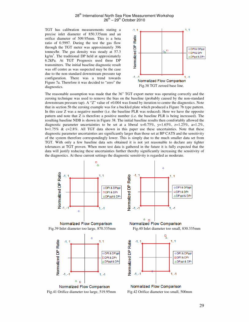
28th International North Sea Flow Measurement Workshop

26th – 29

th October 2010

29

TGT has calibration measurements stating a

precise inlet diameter of 850.335mm and an

orifice diameter of 509.95mm. This is a beta

ratio of 0.5997. During the test the gas flow

through the TGT meter was approximately 396

tonnes/hr. The gas density was steady at 57.3

kg/m3. The traditional DP held at approximately

6.2kPa. At TGT Prognosis used three DP

transmitters. The initial baseline diagnostic result

was off centre as was suspected may be the case

due to the non-standard downstream pressure tap

configuration. There was a trend towards

Figure 7a. Therefore it was decided to “zero” the

diagnostics.

Fig.38 TGT zeroed base line.

The reasonable assumption was made that the 36” TGT export meter was operating correctly and the

zeroing technique was used to remove the bias on the baseline (probably caused by the non-standard

downstream pressure tap). A “Z” value of +0.004 was found by iteration to centre the diagnostics. Note

that in section 5b the zeroing example was for a buckled plate which produced a Figure 7b type pattern.

In this case Z was a negative number (i.e. the baseline PLR was reduced). Here we have the opposite

pattern and note that Z is therefore a positive number (i.e. the baseline PLR is being increased). The

resulting baseline NDB is shown in Figure 38. The initial baseline results then comfortably allowed the

diagnostic parameter uncertainties to be set at a liberal x=0.75%, y=1.65%, z=1.25%, a=1.2%,

b=1.75% & c=2.8%. All TGT data shown in this paper use these uncertainties. Note that these

diagnostic parameter uncertainties are significantly larger than those set at BP CATS and the sensitivity

of the system therefore correspondingly lower. This is simply due to the much smaller data set from

TGT. With only a few baseline data sets obtained it is not yet reasonable to declare any tighter

tolerances at TGT proven. When more test data is gathered in the future it is fully expected that the

data will justify reducing these uncertainties further thereby significantly increasing the sensitivity of

the diagnostics. At these current settings the diagnostic sensitivity is regarded as moderate.

Fig.39 Inlet diameter too large, 870.335mm Fig.40 Inlet diameter too small, 830.335mm

Fig.41 Orifice diameter too large, 519.95mm Fig.42 Orifice diameter too small, 500mm

28th International North Sea Flow Measurement Workshop

26th – 29

th October 2010

30

The initial TGT diagnostic testing carried out so far was for geometry keypad input errors. The inlet

and the orifice diameters were entered with positive and negative errors. Figure 39 shows the

diagnostic response when the inlet diameter of 850.335mm is incorrectly entered as 870.335mm. Such

an error creates an under-reading of the flow by approximately -0.65%. The resulting diagnostic NDB

pattern is compliant with the consequences of the first law of thermodynamics. The pattern is a Figure

7b type suggesting an under-reading may exist. Equation 1 confirmed that the DP’s are measured

correctly. (In examples where the DP’s are read correctly there is no significant difference between the

plots of when the system uses two or three DP transmitters. For this reason only results for three DP

transmitters in use are shown here for the TGT examples.)

Figure 40 shows the result when the inlet diameter is incorrectly entered as 830.335mm. Such an error

creates an over-reading of the flow by approximately +0.75%. The resulting NDB pattern is compliant

with the consequences of the first law of thermodynamics. The pattern is a Figure 7a type suggesting

an over-reading may exist. Equation 1 confirmed that the DP’s are measured correctly. Figure 41

shows the result when the orifice diameter of 509.95mm is incorrectly entered as 519.95mm. Such an

error creates an over-reading of the flow by approximately +4.6%. The resulting NDB pattern is

compliant with the consequences of the first law of thermodynamics. The pattern is a Figure 7a type

suggesting an over-reading may exist. Equation 1 confirmed that the DP’s are measured correctly.

Figure 42 shows the result when the orifice diameter is incorrectly entered as 500mm. Such an error

creates an under-reading of the flow by approximately -4.4%. The resulting NDB pattern is compliant

with the consequences of the first law of thermodynamics. The pattern is a Figure 7b type suggesting

an under-reading may exist. Equation 1 confirmed that the DP’s are measured correctly.

The initial TGT field trials on Prognosis have given the same general results as those from BP CATS.

Prognosis correctly signalled a warning for the cases of the four geometry keypad entry errors. The

system indicated that the DP transmitters were operating correctly and suggested the bias of the

indicated mis-measurement. As with BP CATS it was found that the diagnostics were extremely

sensitive to inlet diameter errors but moderately sensitive to orifice diameter errors. However, it should

be noted that it is expected that continued testing at TGT will allow the baseline diagnostic parameters

to be considerably reduced and the systems sensitivity significantly increased.

Conclusions

In 2008 and 2009 DP Diagnostics proposed a diagnostic methodology for orifice meters based on

theoretical principles and laboratory testing of 4” orifice meters. Swinton Technology has now

developed an industrial product called Prognosis that allows these principles to be applied in practice to

industrial orifice meters. DP Diagnostics has since successfully tested the diagnostics method at the

CEESI Iowa laboratory on a large (16”) orifice plate meter. DP Diagnostics and Swinton Technology

have now successfully tested Prognosis on a large orifice meter at the BP CATS gas terminal and have

initiated testing on a large orifice meter at the ConocoPhillips Theddlethorpe gas terminal.

It has been found that the diagnostics are sensitive to all induced metering problems investigated.

However, the diagnostics have different levels of sensitivity to different meter problems. These range

from extremely to moderately sensitive. For example, an inlet diameter keypad entry error producing a

very small flow rate error produces a very clear diagnostic warning, i.e. the points are far outside the

NDB. At the other extreme, an orifice diameter keypad entry error producing a moderate flow rate

error produces a relatively small diagnostic warning, i.e. the points are just outside the NDB.

Nevertheless, study of the substantial data taken at BP CATS strongly suggests that the majority of

metering problems can be seen by the diagnostics before the flow rate error exceeds ±1%. Of all the

potential problems an orifice meter can face it appears the diagnostics are least sensitive to the keypad

entry error of the orifice diameter. Case studies at BP CATS so far confirm that the diagnostics will

still see an orifice diameter keypad entry induced flow rate error definitely within 1.5% and probably to

within 1.0%. All other issues are more sensitive to the diagnostics and smaller errors can be identified.

Prognosis was developed to help identify when an orifice meter has a malfunction. However, BP CATS

have suggested another use for Prognosis. Custody transfer orifice meters for natural gas that currently

have no diagnostics are regularly scrutinized with scheduled routine maintenance. These requirements

place a financial burden on the meter operator. In most cases the routine maintenance shows that the

meter had been fully serviceable, and the costly maintenance was only necessary to assure all interested

parties of this. This routine maintenance takes time and money and removes the system from the

service it is required for. Furthermore, maintenance requires the meter run be isolated and the gas

28th International North Sea Flow Measurement Workshop

26th – 29

th October 2010

31

blown down to the atmosphere which has an environmental cost. There is also a safety issue associated

with maintenance with personnel regularly operating on high pressure systems. Therefore BP CATS

consider a major potential use for Prognosis to be showing that the meter does not have a problem and

hence preventative maintenance checks can be reduced in frequency. This would offer financial

savings with reduced maintenance costs, reduce the quantity of gas released to the environment and

reduce the exposure of the personnel to the hazardous environment of the high pressure system.

References

1. Steven, R. “Diagnostic Methodologies for Generic Differential Pressure Flow Meters”, North Sea

Flow Measurement Workshop October 2008, St Andrews, Scotland, UK.

2. Steven, R. “Significantly Improved Capabilities of DP Meter Diagnostic Methodologies”, North Sea

Flow Measurement Workshop October 2009, Tonsberg, Norway.

3. International Standard Organisation, “Measurement of Fluid Flow by Means of Pressure Differential

Devices, Inserted in circular cross section conduits running full”, no. 5167, 2003.