6.883 Learning with Combinatorial StructureNote for Lecture 21

Author: Swati Gupta

The last few lectures have been about online combinatorial optimization, learning ban-dits, etc. Today we will switch gears to talk about probabilistic models of diversity. Thesemodels increase the probability of sets that are more spread out and diverse. For example,consider the problem of detecting where the people are in a given picture. Ideally, youwould expect people to be spatially far from each other, and not standing on top of eachother. We want probabilistic models that capture negative correlations, i.e., including anelement a makes it less likely to include another element b.

1 Determinantal Point Processes

Determinantal point processes (DPP) are elegant probabilistic models that capture nega-tive correlation and admit efficient algorithms for sampling, marginalization, condition-ing, etc. These processes were first studied by [8], as fermion processes, to model the distri-bution of fermions at thermal equilibrium. The specific term ‘determinantal’ was coinedby [2] and has since then been used widely. A point process P on the ground set V is aprobability measure on the power set of V , i.e., 2V .

Definition 1 A point process P is called a determinantal point process, if Y is a randomsubset drawn according to P , then we have for every S ⊆ Y ,

P (S ⊆ Y ) = det(KS), (1)

for some similarity matrix K ∈ Rn×n that is symmetric, real and positive semidefinite.Here, KS denotes the submatrix of K obtained by restricting to rows and columns in-dexed in S.

Since the marginal probabilities of any set S ⊆ V must lie in [0, 1], we require every prin-cipal minor of det(KS) ofK must be nonnegative, henceK must be positive semidefinite.It can be shown that the eigenvalues of K must lie between 0 and 1, i.e., 0 � K � 1. (Infact, these conditions are sufficient: any K such that 0 � K � 1 defines a DPP). K is oftenreferred to as the marginal kernel.

Note that P (ei ∈ Y ) = Kii, i.e., the marginal probability of including that element.Now, the marginal probability of including two elements, say ei and ej , is given byP (ei, ej ∈ Y ) = KiiKjj − K2

ij = P (ei ∈ Y )P (ej ∈ Y ) − K2ij . Since K is positive semi-

definite, Kij is non-negative and hence we’ve modeled repulsion. A larger value of Kij

1

implies that i and j are more likely to not appear together. Further, note that if the kernelmatrix K is diagonal, then P (S ⊆ Y ) = det(diag(p1, p2, . . . , p|S|)) = Πi∈Spi. Thus, wecan model independent point processes using DPPs. However, the correlation betweenany two elements is always non-negative for DPPs and one cannot model positive corre-lation.

1.1 Examples

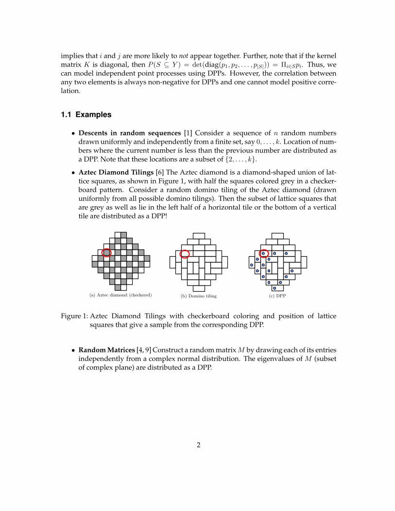
• Descents in random sequences [1] Consider a sequence of n random numbersdrawn uniformly and independently from a finite set, say 0, . . . , k. Location of num-bers where the current number is less than the previous number are distributed asa DPP. Note that these locations are a subset of {2, . . . , k}.• Aztec Diamond Tilings [6] The Aztec diamond is a diamond-shaped union of lat-

tice squares, as shown in Figure 1, with half the squares colored grey in a checker-board pattern. Consider a random domino tiling of the Aztec diamond (drawnuniformly from all possible domino tilings). Then the subset of lattice squares thatare grey as well as lie in the left half of a horizontal tile or the bottom of a verticaltile are distributed as a DPP!

�0�%($�+�' ����+�

•  Aztec'diamonds

•  draw'a'domino'4ling'uniformly'at'random •  Let'S'='{'gray'squares'that'are'the'le`'half'of'some'4le'}

•  S'is'distributed'as'a'DPP!'

(a) Aztec diamond (checkered) (b) Domino tiling (c) DPP

Figure 5: Aztec diamonds.

2.2 L-ensembles

For the purposes of modeling real data, it is useful to slightly restrict the class of DPPsby focusing on L-ensembles. First introduced by Borodin and Rains [2005], an L-ensembledefines a DPP not through the marginal kernel K, but through a real, symmetric matrix Lindexed by the elements of Y:

PL(Y = Y ) / det(LY ) . (6)

Whereas Equation (1) gave the marginal probabilities of inclusion for subsets A, Equation (6)directly specifies the atomic probabilities for every possible instantiation of Y . As for K, itis easy to see that L must be positive semidefinite. However, since Equation (6) is only astatement of proportionality, the eigenvalues of L need not be less than one; any positivesemidefinite L defines an L-ensemble. The required normalization constant can be given inclosed form due to the fact that

PY ✓Y det(LY ) = det(L + I), where I is the N ⇥N identity

matrix. This is a special case of the following theorem.

Theorem 2.1. For any A ✓ Y,

X

A✓Y ✓Ydet(LY ) = det(L + IA) , (7)

where IA is the diagonal matrix with ones in the diagonal positions corresponding to elementsof A = Y �A, and zeros everywhere else.

Proof. Suppose that A = Y ; then Equation (7) holds trivially. Now suppose inductively thatthe theorem holds whenever A has cardinality less than k. Given A such that |A| = k > 0,let i be an element of Y where i 2 A. Splitting blockwise according to the partitionY = {i} [ Y � {i}, we can write

L + IA =

✓Lii + 1 Lii

Lii LY�{i} + IY�{i}�A

◆, (8)

8

(a) Aztec diamond (checkered) (b) Domino tiling (c) DPP

Figure 5: Aztec diamonds.

2.2 L-ensembles

For the purposes of modeling real data, it is useful to slightly restrict the class of DPPsby focusing on L-ensembles. First introduced by Borodin and Rains [2005], an L-ensembledefines a DPP not through the marginal kernel K, but through a real, symmetric matrix Lindexed by the elements of Y:

PL(Y = Y ) / det(LY ) . (6)

Whereas Equation (1) gave the marginal probabilities of inclusion for subsets A, Equation (6)directly specifies the atomic probabilities for every possible instantiation of Y . As for K, itis easy to see that L must be positive semidefinite. However, since Equation (6) is only astatement of proportionality, the eigenvalues of L need not be less than one; any positivesemidefinite L defines an L-ensemble. The required normalization constant can be given inclosed form due to the fact that

PY ✓Y det(LY ) = det(L + I), where I is the N ⇥N identity

matrix. This is a special case of the following theorem.

Theorem 2.1. For any A ✓ Y,

X

A✓Y ✓Ydet(LY ) = det(L + IA) , (7)

where IA is the diagonal matrix with ones in the diagonal positions corresponding to elementsof A = Y �A, and zeros everywhere else.

Proof. Suppose that A = Y ; then Equation (7) holds trivially. Now suppose inductively thatthe theorem holds whenever A has cardinality less than k. Given A such that |A| = k > 0,let i be an element of Y where i 2 A. Splitting blockwise according to the partitionY = {i} [ Y � {i}, we can write

L + IA =

✓Lii + 1 Lii

Lii LY�{i} + IY�{i}�A

◆, (8)

8

(a) Aztec diamond (checkered) (b) Domino tiling (c) DPP

Figure 5: Aztec diamonds.

2.2 L-ensembles

For the purposes of modeling real data, it is useful to slightly restrict the class of DPPsby focusing on L-ensembles. First introduced by Borodin and Rains [2005], an L-ensembledefines a DPP not through the marginal kernel K, but through a real, symmetric matrix Lindexed by the elements of Y:

PL(Y = Y ) / det(LY ) . (6)

Whereas Equation (1) gave the marginal probabilities of inclusion for subsets A, Equation (6)directly specifies the atomic probabilities for every possible instantiation of Y . As for K, itis easy to see that L must be positive semidefinite. However, since Equation (6) is only astatement of proportionality, the eigenvalues of L need not be less than one; any positivesemidefinite L defines an L-ensemble. The required normalization constant can be given inclosed form due to the fact that

PY ✓Y det(LY ) = det(L + I), where I is the N ⇥N identity

matrix. This is a special case of the following theorem.

Theorem 2.1. For any A ✓ Y,

X

A✓Y ✓Ydet(LY ) = det(L + IA) , (7)

where IA is the diagonal matrix with ones in the diagonal positions corresponding to elementsof A = Y �A, and zeros everywhere else.

Proof. Suppose that A = Y ; then Equation (7) holds trivially. Now suppose inductively thatthe theorem holds whenever A has cardinality less than k. Given A such that |A| = k > 0,let i be an element of Y where i 2 A. Splitting blockwise according to the partitionY = {i} [ Y � {i}, we can write

L + IA =

✓Lii + 1 Lii

Lii LY�{i} + IY�{i}�A

◆, (8)

8

(K.)Johansson.)The)arcDc)circle)boundary)and)the)airy)process))2005)

Figure 1: Aztec Diamond Tilings with checkerboard coloring and position of latticesquares that give a sample from the corresponding DPP.

• Random Matrices [4, 9] Construct a random matrixM by drawing each of its entriesindependently from a complex normal distribution. The eigenvalues of M (subsetof complex plane) are distributed as a DPP.

2

1.2 L-ensembles

L-ensembles, introduced by Borodin and Rains in 2005 [3], are a slightly restricted buta useful class of DPPs. They are defined using a real, symmetric matrix L indexed bythe elements of V . The unnormalized probability of sampling a set of Y ⊆ V is givenby

PL(Y ) ∝ det(LY ). (2)

This immediately justifies that L � 0. The natural question at this point is, can we computethe normalization constant for an L-ensemble? The normalization constant is simply the sumof the unnormalized probabilities over all subsets of the V , i.e.

∑S⊆V det(LS), and the

following theorem shows that normalization is tractable (as opposed to graphical models,computing normalization reduces to linear algebra for DPPs).

Theorem 1. For any A ⊆ V :∑

A⊆Y⊆Vdet(LY ) = det(L+ IA),

where IA is a diagonal matrix such that Iii = 0 for indices i ∈ A and Iii = 1 for i ∈ A.

Proof. By induction on the size ofA and expanding the determinant in the induction step.See Theorem 2.1, on Page 8 of Kulesza and Taskar’s survey [7] on Determinantal pointprocesses for machine learning for the full proof.

Setting A = φ, we obtain the following corollary:

Corollary 1. The normalization constant of an L-ensemble is given by∑

S⊆Vdet(LS) = det(L+ IV).

Equivalence of the two definitions There is a very close relation between DPPs de-fined using the marginal kernel K and L-ensembles, and it is precisely quantified by thefollowing result of Macchi [8].

Theorem 2. An L-ensemble is a DPP, and its marginal kernel isK = L(L+I)−1 = I−(L+I)−1.

3

Proof. Using Theorem 1, the marginal probability of a set A ⊆ V under the L-ensemble is

PL(A ⊆ Y ) =

∑Y :A⊆Y⊆V det(LY )∑

Y⊆V detLY(3)

=det(L+ IA)

det(L+ I)(4)

= det((L+ IA)(L+ I)−1) (5)

= det(IA(L+ I)−1 + I − (L+ I)−1) . . . using L(L+ I)−1 = I − (L+ I)−1

(6)

= det(IA(L+ I)−1 + (IA + IA)(I − (L+ I)−1) (7)= det(IA + IAK) (8)

=

∣∣∣∣I|A|×|A|0KA,AKA

∣∣∣∣ (9)

= det(IA×A) det(KA) = det(KA). (10)

This implies that all the marginals agree, and thus an L-ensemble is equivalent to a DPPwith a marginal kernel K = L(L+ I)−1.

Note that an L-ensemble can be constructed using a marginal kernel K by setting L =K(I − K)−1. Hence, a corresponding L-ensemble exists only if the (I − K) is invert-ible. In this sense, DPPs are slightly more general than L-ensembles. (Existence of a in-verse is equivalent to the point process assigning some nonzero probability to the emptyset).

Eigenvalue Decomposition Suppose the eigendecomposition of L =∑

k λkvkvTk , then

K =∑

kλkλk+1vkv

Tk .

Geometric View Suppose we have some data points such that x1, . . . , xn are the corre-sponding feature vectors in Rd. We can construct an L-ensemble such that Lij = xTi xj .Then,

PL(S) ∝ det(LS) = Vol2({xi}i∈S).

This implies that if a set contains a more diverse set of feature vectors, the volume spannedby them would be greater resulting in a larger probability of sampling such a set. If thedimension of the feature vectors d is less than the number of points, then the samplesfrom the corresponding DPP will only contain at most d points.

4

2 Working with DPPs

One of the primary advantages of DPPs is that, although the number of possible realiza-tions of P is exponential in V , many types of inference can be performed in polynomialtime. We discuss some here.

• Complements If Y ∼ DPP(K), then Y = V \ Y ∼ DPP(I −K). In particular,

P (A ∩ Y = φ) = det(I −KA).

• Conditioning The conditional probability that a set B is observed such that it con-tains elements in Ain and does not contain elements in Aout conditioned on observ-ing Ain and Aout is given by

PL(Y = Ain ∪B|Ain ⊆ Y,Aout ∩ Y = φ) =det(LAin∪B)

det(LAout + IAin).

• Marginals Conditional marginal of B given that A has been observed is given by

P (B ⊆ Y |A ⊆ Y ) = det(KAB)

for KA = I − [(L+ IA)−1]A.

• Scaling If K = γK ′, for some 0 ≤ γ ≤ 1, then for all A ⊆ V , we have det(KA) =γ|A|K ′A.

Computing the mode of a DPP, i.e., finding a set Y ⊆ V that maximizes PL(Y ), is in gen-eral NP-hard. This problem is also sometimes called the maximum a posteriori (MAP) in-ference. We will next look at how one can sample efficiently from DPPs.

2.1 Sampling

There are two important questions with respect to sampling: (i) how to draw a sample,and (ii) how many points there are in a sample. The main idea in sampling DPPs is to viewevery DPP as a mixture of elementary DPPs. A DPP is called elementary if every eigen-value of its marginal kernel is in {0, 1}. P T denotes an elementary DPP with marginalkernel KT =

∑v∈T vv

T , where T is a set of orthonormal vectors.

We will look at the sampling procedure developed by Hough et al. [5], formally presentedin Algorithm 1. This algorithm has two main steps:

• Sample a mixture component P T with probability πT ,

• Sample Y from P T .

5

In the first phase of the algorithm, a subset of the eigenvectors is selected a random,where the probability of selecting each eigenvector vk is λk

λk+1 . In the second phase, thecorresponding elementary DPP (to the eigenvectors selected in the first phase) is sam-pled for a subset Y . We first note that a DPP can be expressed as a mixture of simplerDPPs.

Lemma 1 (Sampling lemma). A DPP with kernel L =∑

k λkvkvTk is a mixture of elemen-

tary DPPs: P T such that PL = 1det(L+I)

∑T⊆V Πk∈TλkP T where V is the set of orthonormal

eigenvectors of L.

Proof. The proof shows that the two distributions agree on all the marginal probabilities.See Lemma 2.6 of [7].

After the first phase has selected a set of eigenvectors A, we sample a subset Y fromthis elementary DPP. It is easier to sample from an elementary DPP, as each sample hascardinality = |A|.

Lemma 2. If Y is drawn according to an elementary DPP PA, then |Y | = |A| with probability1.

Proof. We have E[|Y |] = E[∑n

i=1 1[i ∈ Y ]] =∑n

i=1 P (i ∈ Y ), but this probability is just∑ni=1Ki,i. In general, trace of K gives the expected number of points. In case of elemen-

tary DPPs, the trace of K is exactly the cardinality of A, i.e., tr(K) =∑n

i=1Ki,i = |A|.In the case of elementary DPPs, we don’t even fluctuate away from the expectation sincethe rank is |A|, and thus we cannot sample more than |A|. That is, for any Y, |Y | > |A| :P (Y ) = det(LA) = 0. Hence, we must always sample sets of cardinality exactly |A|.

Now, for sampling an elementary DPP, we start with an empty set Y = φ. In each it-eration i, we pick a point i conditioned on the previous {1, . . . , i − 1} selected points.Using the geometric intuition, this conditioning is equivalent to projecting the remainingeigenvectors onto a subspace orthogonal to {v1, . . . , vi−1}.

3 Applications

3.1 Sampling points on a plane

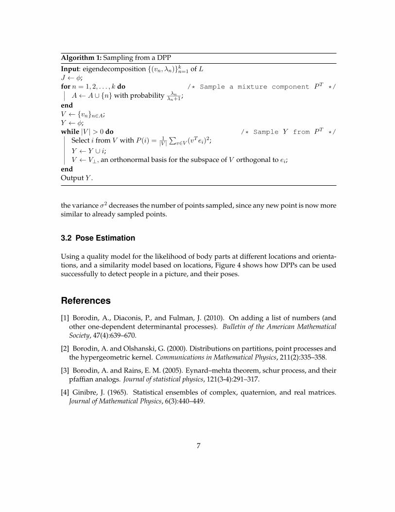
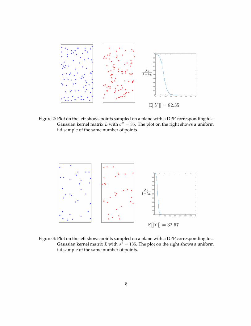
Figures 2 and 3 show the results of sampling from a DPP constructed using a Gaussiankernel with sij = exp(− 1

2σ2 ||xi − xj ||2). Note that there are fewer clusters of points inthe DPP plots, as opposed to uniform iid sampling of the same number of points (asobtained in the DPP sample) in the plots to the right. Also, Figure 3 shows that increasing

6

Algorithm 1: Sampling from a DPP

Input: eigendecomposition {(vn, λn)}kn=1 of LJ ← φ;for n = 1, 2, . . . , k do /* Sample a mixture component P T */

A← A ∪ {n}with probability λnλn+1 ;

endV ← {vn}n∈A;Y ← φ;while |V | > 0 do /* Sample Y from P T */

Select i from V with P (i) = 1|V |∑

v∈V (vT ei)2;

Y ← Y ∪ i;V ← V⊥, an orthonormal basis for the subspace of V orthogonal to ei;

endOutput Y .

the variance σ2 decreases the number of points sampled, since any new point is now moresimilar to already sampled points.

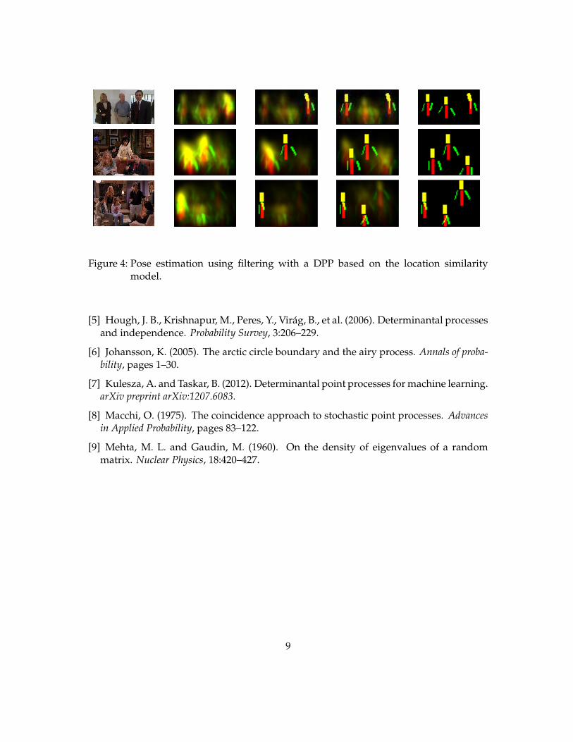
3.2 Pose Estimation

Using a quality model for the likelihood of body parts at different locations and orienta-tions, and a similarity model based on locations, Figure 4 shows how DPPs can be usedsuccessfully to detect people in a picture, and their poses.

References

[1] Borodin, A., Diaconis, P., and Fulman, J. (2010). On adding a list of numbers (andother one-dependent determinantal processes). Bulletin of the American MathematicalSociety, 47(4):639–670.

[2] Borodin, A. and Olshanski, G. (2000). Distributions on partitions, point processes andthe hypergeometric kernel. Communications in Mathematical Physics, 211(2):335–358.

[3] Borodin, A. and Rains, E. M. (2005). Eynard–mehta theorem, schur process, and theirpfaffian analogs. Journal of statistical physics, 121(3-4):291–317.

[4] Ginibre, J. (1965). Statistical ensembles of complex, quaternion, and real matrices.Journal of Mathematical Physics, 6(3):440–449.

7

��%($#&!��0�%($��

•  similarity'measure'L:'Gaussian'kernel sij = exp(� 1

2�2 kxi � xjk2) �2 = 35

0 50 100 150 200 250 300 350 4000

0.1

0.2

0.3

0.4

0.5

0.6

0.7

0.8

0.9

1

�k

1+�k

E[|Y |] = 82.35

Figure 2: Plot on the left shows points sampled on a plane with a DPP corresponding to aGaussian kernel matrix L with σ2 = 35. The plot on the right shows a uniformiid sample of the same number of points.

E[|Y |] = 32.67

50 100 150 200 250 300 350 4000

0.1

0.2

0.3

0.4

0.5

0.6

0.7

0.8

0.9

1

��%($#&!��0�%($��

•  Gaussian'kernel'L sij = exp(� 1

2�2 kxi � xjk2) �2 = 135

�k

1+�k

Figure 3: Plot on the left shows points sampled on a plane with a DPP corresponding to aGaussian kernel matrix L with σ2 = 135. The plot on the right shows a uniformiid sample of the same number of points.

8

�'+���+,#%�,#'&�

Figure 22: Structured marginals for the pose estimation task, visualized as clouds, onsuccessive steps of the sampling algorithm. Already selected poses are superimposed. Inputimages are shown on the left.

95

Figure 4: Pose estimation using filtering with a DPP based on the location similaritymodel.

[5] Hough, J. B., Krishnapur, M., Peres, Y., Virág, B., et al. (2006). Determinantal processesand independence. Probability Survey, 3:206–229.

[6] Johansson, K. (2005). The arctic circle boundary and the airy process. Annals of proba-bility, pages 1–30.

[7] Kulesza, A. and Taskar, B. (2012). Determinantal point processes for machine learning.arXiv preprint arXiv:1207.6083.

[8] Macchi, O. (1975). The coincidence approach to stochastic point processes. Advancesin Applied Probability, pages 83–122.

[9] Mehta, M. L. and Gaudin, M. (1960). On the density of eigenvalues of a randommatrix. Nuclear Physics, 18:420–427.

9