Embed Size (px)
Citation preview

1
Data and central tendency
Integrated Disease Surveillance Programme (IDSP) district surveillance
officers (DSO) course

2
Outline of the session
1. Type of data2. Central tendency

3
Epidemiological process
• We collect data We use criteria and definitions
• We analyze data into information “Data reduction / condensation”
• We interpret the information for decision making What does the information means to us?

4
Surveillance: A role of the public health
systemThe systematic process of collection, transmission,
analysis and feedback of public health data for decision making
Surveillance
Data Information Action
Analysis Interpretation
Today we will focus on DATA: The starting point

5
Data: A definition
• Set of related numbers• Raw material for statistics• Example:
Temperature of a patient over time Date of onset of patients

6
Types of data
• Qualitative data No magnitude / size Classified by counting the units that have the same attribute
Types• Binary • Nominal• Ordinal
• Quantitative data

7
Qualitative, binary data
• The variable can only take two values 1,0 often used (or 1,2) Yes, No
• Example: Sex
• Male, Female
Female sex• Yes, No

8
REC SEX--- ---- 1 M 2 M 3 M 4 F 5 M 6 F 7 F 8 M 9 M 10 M 11 F 12 M 13 M 14 M 15 F 16 F 17 F 18 M 19 M 20 M 21 F 22 M 23 M 24 F 25 M 26 M 27 M 28 F 29 M 30 M
Sex Frequency Proportion
Female 10 33.3%
Male 20 66.7%
Total 30 100.0%
Frequency distribution for a qualitative binary
variable

9
Using a pie chart to display qualitative binary variable
FemaleMale
Distribution of cases by sex

10
Qualitative, nominal data
• The variable can take more than two values Any value
• The information fits into one of the categories
• The categories cannot be ranked• Example:
Nationality Language spoken Blood group

11
Rec State 1 Punjab2 Bihar3 Rajasthan4 Punjab5 Bihar6 Punjab7 Bihar8 Bihar9 UP10 Rajasthan11 Bihar12 Rajasthan13 Punjab14 UP15 Rajasthan16 UP17 Punjab18 UP19 Rajasthan20 Bihar21 UP22 Bihar23 UP24 Rajasthan25 Bihar26 Bihar27 Bihar28 UP29 Bihar30 UP
Country Frequency Proportion
Bihar 11 36.7%
UP 8 26.7%
Rajasthan
6 20.0%
Punjab 5 16.6%
Total 30 100.0%
Frequency distribution for a qualitative nominal
variable

12
Using a horizontal bar chart to display qualitative nominal
variable
0 5 10 15
Punjab
RJ
UP
Bihar
Frequency
Distribution of cases by state

13
Qualitative, ordinal data
• The variable can only take a number of value than can be ranked through some gradient
• Example: Birth order
• First, second, third … Severity
• Mild, moderate, severe Vaccination status
• Unvaccinated, partially vaccinated, fully vaccinated

14
REC Status --- ------- 1 1 2 1 3 2 4 2 5 1 6 2 7 1 8 2 9 3 10 2 11 1 12 3 13 1 14 3 15 1 16 3 17 1 18 1 19 3 20 1 21 1 22 2 23 1 24 2 25 2 26 1 27 2 28 3 29 2 30 2
Clinical status: 1: Mild; 2 : Moderate; 3 : Severe
Frequency distribution for a qualitative ordinal
variableSeverity Frequency Proportion
Mild 13 43.3%
Moderate 11 36.7%
Severe 6 20.0%
Total 30 100.0%

15
0
5
10
15
Mild Moderate Severe
Frequency
Using a vertical bar chart to display qualitative ordinal
variable
Distribution of cases by severity

16
Key issues
• Qualitative data• Quantitative data
We are not simply counting We are also measuring
• Discrete• Continuous

17
Quantitative, discrete data
• Values are distinct and separated• Normally, values have no decimals• Example:
Number of sexual partners Parity Number of persons who died from measles

18
REC CHILDREN--- ------- 1 1 2 2 3 5 4 6 5 3 6 4 7 1 8 1 9 2 10 3 11 1 12 2 13 7 14 3 15 4 16 2 17 1 18 1 19 1 20 1 21 2 22 3 23 1 24 4 25 2 26 1 27 6 28 4 29 3 30 1
Frequency distribution for a quantitative, discrete
dataChildren Frequency Proportion
1 11 36.7%
2 6 20.0%
3 5 16.7%
4 4 13.3%
5 1 3.3%
6 2 6.7%
7 1 3.3%
Total 30 100.0%

19
0
2
4
6
8
10
12
1 2 3 4 5 6 7
Number of children
Frequency
Distribution of households by number of children
Using a histogram to display a discrete quantitative variable

20
Quantitative, continuous data
• Continuous variable• Can assume continuous uninterrupted range of values
• Values may have decimals• Example:
Weight Height Hb level What about temperature?

21
REC WEIGHT --- ------ 1 10.5 2 23.7 3 21.8 4 33.1 5 38.0 6 34.5 7 38.5 8 38.4 9 30.1 10 34.7 11 37.9 12 38.0 13 39.2 14 30.1 15 43.2 16 45.7 17 40.4 18 56.4 19 55.1 20 55.4 21 66.7 22 82.9 23 109.7 24 120.2 25 10.4 26 10.8 27 25.5 28 20.2 29 27.3 30 38.7
Weight Tally mark Frequency
10-19 III 3
20-29 IIIII 5
30-39 IIIII IIIII II
12
40-49 III 3
50-59 III 3
60-69 I 1
70-79 - 0
80-89 I 1
90-99 - 0
100-109 I 1
110-119 I 1
Frequency distribution for a continuous quantitative variable: The tally mark

22
REC WEIGHT --- ------ 1 10.5 2 23.7 3 21.8 4 33.1 5 38.0 6 34.5 7 38.5 8 38.4 9 30.1 10 34.7 11 37.9 12 38.0 13 39.2 14 30.1 15 43.2 16 45.7 17 40.4 18 56.4 19 55.1 20 55.4 21 66.7 22 82.9 23 109.7 24 120.2 25 10.4 26 10.8 27 25.5 28 20.2 29 27.3 30 38.7
Weight Frequency
Proportion
10-19 3 10.0%
20-29 5 16.7%
30-39 12 40.0%
40-49 3 10.0%
50-59 3 10.0%
60-69 1 3.3%
70-79 0 0.0%
80-89 1 3.3%
90-99 0 0.0%
100-109 1 3.3%
110-119 1 3.3%
Total 30 100.0%
Frequency distribution for a continuous quantitative
variable, after aggregation

23
Using a histogram to display a frequency distribution for a
continuous quantitative variable, after aggregation
0
2
4
6
8
10
12
14
0-9 ハ 10-19 20-29 30-39 40-49 50-59 60-69 70-79 80-89 90-99 100-9 110-9
Weight categories
Frequency
Distribution of cases by weight

24
Summary statistics
• A single value that summarizes the observed value of a variable Part of the data reduction process
• Two types: Measures of location/central tendency/average Measures of dispersion/variability/spread
• Describe the shape of the distribution of a set of observations
• Necessary for precise and efficient comparisons of different sets of data The location (average) and shape (variability) of different distributions may be different

250
5
10
15
20
0-9 10-19 20-29 30-39 40-49 50-59 60-69 70-79 80-89 90-99
Position
Dispersion
Describing a distribution

26
No. ofPeople
Factor X
Population A
Population B
Different VariabilitySame Location
Same location, different variability

27
Different location, same variability
28
Measures of central tendency
• Mode • Median • Arithmetic mean

29
The mode
• Definition The mode of a distribution is the value that is observed most frequently in a given set of data
• How to obtain it? Arrange the data in sequence from low to high
Count the number of times each value occurs
The most frequently occurring value is the mode

30
The mode
0
2
4
6
8
10
12
14
16
18
20
N
Mode

31
Examples of mode annual salary
(in 10,000 rupees) • 4, 3, 3, 2, 3, 8, 4, 3, 7, 2• Arranging the values in order:
2, 2, 3, 3, 3, 3, 4, 4, 7, 8 7, 8 The mode is three times “3”

32
Specific features of the mode
• There may be no mode When each value is unique
• There may be more than one mode When more than 1 peak occurs Bimodal distribution
• The mode is not amenable to statistical tests
• The mode is not based on all the observations

33
The median
• The median describes literally the middle value of the data
• It is defined as the value above or below which half (50%) the observations fall

34
Computing the median
• Arrange the observations in order from smallest to largest (ascending order) or vice-versa
• Count the number of observations “n” If “n” is an odd number
• Median = value of the (n+1) / 2th observation(Middle value)
If “n” is an even number• Median = the average of the n / 2th and (n /2)+1th observations(Average of the two middle numbers)

35
Example of median calculation
• What is the median of the following values: 10, 20, 12, 3, 18, 16, 14, 25, 2 Arrange the numbers in increasing order
• 2 , 3, 10, 12, 14, 16, 18, 20, 25• Median = 14
• Suppose there is one more observation (8) 2 , 3, 8, 10, 12, 14, 16, 18, 20, 25
Median = Mean of 12 & 14 = 13

36
Advantages and disadvantages of the median
• Advantages The median is unaffected by extreme values
• Disadvantages The median does not contain information on the other values of the distribution • Only selected by its rank• You can change 50% of the values without affecting the median
The median is less amenable to statistical tests

37
Median
0
2
4
6
8
10
12
14
Class of the variable
0
2
4
6
8
10
12
14
Class of the variable
The median is not sensitive to
extreme values
Same median

38
Mean (Arithmetic mean / Average)
• Most commonly used measure of location• Definition
Calculated by adding all observed values and dividing by the total number of observations
• Notations Each observation is denoted as x1, x2, … xn
The total number of observations: n Summation process = Sigma : The mean: X
X = xi /n

39
Computation of the mean
• Duration of stay in days in a hospital 8,25,7,5,8,3,10,12,9
• 9 observations (n=9)• Sum of all observations = 87• Mean duration of stay = 87 / 9 = 9.67
• Incubation period in days of a disease 8,45,7,5,8,3,10,12,9
• 9 observations (n=9)• Sum of all observations =107 • Mean incubation period = 107 / 9 = 11.89

40
Advantages and disadvantages of the mean
• Advantages Has a lot of good theoretical properties Used as the basis of many statistical tests
Good summary statistic for a symmetrical distribution
• Disadvantages Less useful for an asymmetric distribution• Can be distorted by outliers, therefore giving a less “typical” value

41
0
2
4
6
8
10
12
14
N
Mean = 10.8
0 1 2 3 4 5 6 7 8 9 10 11 12 13 14 15 16 17 18 19
Median = 10 Mode = 13.5
42
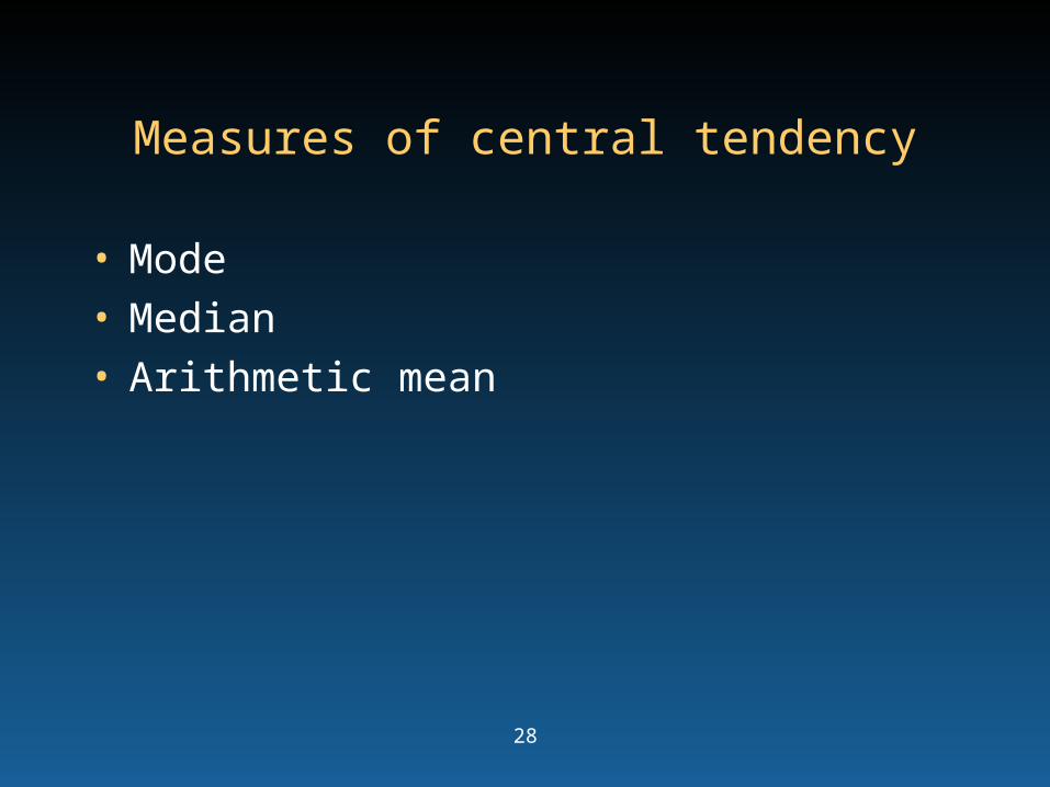
Ideal characteristics of a measure of central tendency
• Easy to understand• Simple to compute• Not unduly affected by extreme values• Rigidly defined
Clear guidelines for calculation
• Capable of further mathematical treatment
• Sample stability Different samples generate same measure

43
What measure of location to use?
• Consider the duration (days) of absence from work of 21 labourers owing to sickness 1, 1, 2, 2, 3, 3, 4, 4, 4, 4, 5, 6, 6, 6, 7, 8, 9, 10, 10, 59, 80
• Mean = 11 days Not typical of the series as 19 of the 21 labourers were absent for less than 11 days
Distorted by extreme values
• Median = 5 days Better measure

44
Type of data: Summary
Qualitative
Binary Nominal Ordinal
Sex State Status M Bihar MildM Punjab ModerateF Bihar SevereM Punjab MildF UP ModerateF Bihar MildM UP ModerateM Rajasthan SevereF Punjab SevereM Rajasthan MildF Bihar ModerateF UP ModerateM Rajasthan MildM Bihar SevereM Punjab SevereF Punjab ModerateM Rajasthan MildF UP MildM Bihar Mild
Quantitative
Discrete Continuous
Children Weight 1 56.41 47.82 59.93 13.11 25.71 23.02 30.03 13.72 15.42 52.51 26.61 38.21 59.02 57.92 19.63 31.72 15.13 33.91 45.6
45
Definitions of measures of central tendency
• Mode The most frequently occuring observation
• Median The mid-point of a set of ordered observations
• Arithmetic mean Aggregate / sum of the given observations divided by the number of observation


![INTEGRATED DISEASE SURVEILLANCE PROGRAMME (IDSP) [Compatibility Mode].pdf · Integrated Disease Surveillance Programme ... – Form P (Probable Cases): Doctors ... S,P,L forms & EWS](https://img.pdfslide.us/doc/110x75/5b1d22937f8b9a16788c006b/integrated-disease-surveillance-programme-idsp-compatibility-modepdf-integrated.jpg)