Embed Size (px)
Citation preview
1
CUTTING PERFORMANCE AND STABILITY OF HELICAL ENDMILLS WITH
VARIABLE PITCH
By
KEVIN BRADY POWELL
A THESIS PRESENTED TO THE GRADUATE SCHOOL OF THE UNIVERSITY OF FLORIDA IN PARTIAL FULFILLMENT
OF THE REQUIREMENTS FOR THE DEGREE OF MASTER OF SCIENCE
UNIVERSITY OF FLORIDA
2008

2
Copyright 2008
by
Kevin Brady Powell

3
ACKNOWLEDGMENTS
I would like to thank my parents and the rest of my family, for their love, support, and
encouragement. Their success in life has been a constant inspiration. I would like to extend a
most heartfelt thanks to Amber Wangle her love has been a great motivator.
I would also like to extend a special thanks to Dr. Tony L. Schmitz for giving me the
opportunity to work in a great research environment. His endless enthusiasm and exceptional
knowledge always made it easy to come to work. I would also like to thank the rest of my
committee, Dr. John K. Schueller and Dr. Gloria J. Wiens. A big thanks goes to Dr. Hitomi
Yamaguchi Greenslet and the members of the Machine Tool Research Center whose assistance
and friendship proved to be invaluable, especially Raul Zapata who helped in the development of
the peak-to-peak stability lobe diagram.
This work would not have been possible without support from Thomas Long and Srikanth
Bontha of Kennametal, Inc.
4
TABLE OF CONTENTS page
ACKNOWLEDGMENTS ...............................................................................................................3
LIST OF TABLES...........................................................................................................................6
LIST OF FIGURES .........................................................................................................................7
ABSTRACT...................................................................................................................................10
CHAPTER
1 INTRODUCTION ...................................................................................................................12
2 LITERATURE REVIEW.........................................................................................................14
Self-Excited Vibrations in Machining (Chatter).....................................................................14 Prediction and Modeling of Machining Stability ...................................................................14 Tool Geometry in Machining Stability...................................................................................15
3 CUTTING FORCE MODEL ...................................................................................................16
Development...........................................................................................................................16 Determination .........................................................................................................................16
4 TIME DOMAIN SIMULATION ............................................................................................22
Description..............................................................................................................................22 Verification .............................................................................................................................23
5 PEAK-TO-PEAK STABILITY LOBE IMPLEMENTATION ..............................................25
6 PEAK-TO-PEAK STABILITY LOBE VERIFICATION ......................................................30
Uniform and Variable Pitch Peak-to-Peak Stability Lobe Comparison .................................30 Experimental Setup and Procedure.........................................................................................31
Cutting Tests....................................................................................................................31 Flexure Design.................................................................................................................32 Stability Determination ...................................................................................................33
7 STABILITY LOBE VERIFICATION RESULTS ..................................................................42
8 CONCLUSION .......................................................................................................................46
APPENDIX
A ONCE-PER-REVOLUTION PLOTS ......................................................................................50

5
B MATLAB TIME DOMAIN SIMULATION CODE................................................................62
LIST OF REFERENCES ...............................................................................................................69
BIOGRAPHICAL SKETCH .........................................................................................................71

6
LIST OF TABLES
Table page 3-1: Cutting tests to determine cutting force coefficients..............................................................20
3-2: Cutting force coefficients (Kennametal HEC750S4).............................................................21

7
LIST OF FIGURES
Figure page 3-1: Cutting force model. ...............................................................................................................17
3-2: Cutting force coefficient test setup. ........................................................................................18
3-3: Mean cutting force versus feed rate (2000 rpm, ADOC = 2 mm) ..........................................18
3-4: Mean cutting force versus feed rate (6000 rpm, ADOC = 2 mm) ..........................................19
3-5: Mean cutting force versus feed rate (10,000 rpm, ADOC = 2 mm) .......................................19
3-6: Mean cutting force versus feed rate (15,000 rpm, ADOC = 2 mm) .......................................20
4-1 Time domain simulation results for an endmill with variable pitch at 25% radial immersion. .........................................................................................................................24
5-1: Chip thickness variation due to cutter vibrations....................................................................25
5-2: Force versus time for a tool with uniform pitch at 7200 rpm and a 4 mm axial depth-of-cut (unstable cutting, chatter)..............................................................................27
5-3: Force versus time for a tool with variable pitch at 7200 rpm and a 4 mm axial depth-of-cut (stable cutting)...............................................................................................27
5-4: Peak-to-peak force plot for a tool with uniform pitch. ..........................................................28
5-5: Analytical stability lobes [10]. ...............................................................................................28
5-6: Peak-to-peak stability lobes (uniform pitch)..........................................................................29
6-1: Endmill geometry. A) Uniform pitch (Kennametal HEC750S4). B) Variable pitch.............30
6-2: Peak-to-peak force plot (uniform pitch 1:10 mm x .25 mm) .................................................34
6-3: Peak-to-peak stability lobes (uniform pitch)..........................................................................34
6-4: Peak-to-peak force plot (variable pitch 1:10 mm x .25 mm). ................................................35
6-5: Peak-to-peak stability lobes (variable pitch)..........................................................................35
6-6: Peak-to-peak force plot (uniform pitch, 1:10 mm x .25 mm) ................................................36
6-7: Peak-to-peak stability lobes (uniform pitch)..........................................................................36
6-8: Peak-to-peak force plot (variable pitch, 1:10 mm x .25 mm) ................................................37

8
6-9: Peak-to-peak stability lobes (variable pitch)..........................................................................37
6-10: Flexure-based cutting test setup...........................................................................................38
6-11: Cutting stability setup. .........................................................................................................38
6-12: Key notch-style flexure dimensions (in mm).......................................................................39
6-13: Flexure model mesh for modal analysis. .............................................................................39
6-14: Flexure FEM model. a) Sinusoidal force along the top edge. b) Bottom face constrained in all DOF’s. c) FRF determined at top edge. ................................................40
6-15: Flexure and tool-tip frequency response functions. .............................................................40
6-16: Stable cutting vibration (variable pitch, 7300 rpm, 4 mm axial depth-of-cut) ....................41
6-17: Unstable cutting vibration (uniform pitch, 7300 rpm, 4 mm axial depth-of-cut) ................41
7-1: Peak-to-peak stability lobes with experimental results (uniform pitch). ...............................43
7-2: Peak-to-peak stability lobes with experimental results (variable pitch). ...............................43
7-3: Uniform pitch, 7300 rpm, 2.5 mm depth of cut (stable). .......................................................44
7-4: Uniform pitch, 7300 rpm, 3 mm depth of cut (unstable). ......................................................44
7-5: Variable pitch, 7300 rpm, 4 mm depth of cut (stable). ..........................................................45
7-6: Variable pitch, 7300 rpm, 4.5 mm depth of cut (unstable). ...................................................45
8-1: Workpiece chips welded to cutting teeth ...............................................................................48
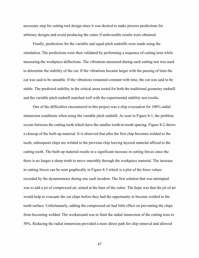
8-2: Close up of welded chips .......................................................................................................49
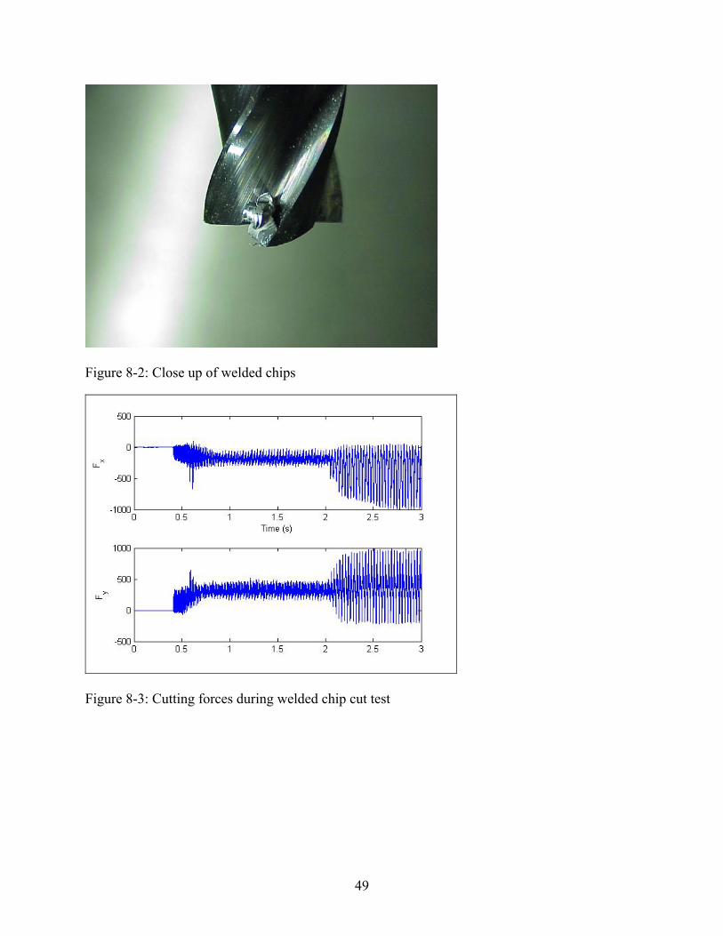
8-3: Cutting forces during welded chip cut test.............................................................................49
A-1: Uniform pitch, 7225 rpm, 2 mm depth of cut. ......................................................................50
A-2: Uniform pitch, 7225 rpm, 2.5 mm depth of cut. ...................................................................50
A-3: Uniform pitch, 7225 rpm, 3 mm depth of cut. ......................................................................51
A-4: Uniform pitch, 7225 rpm, 3.5 mm depth of cut. ...................................................................51
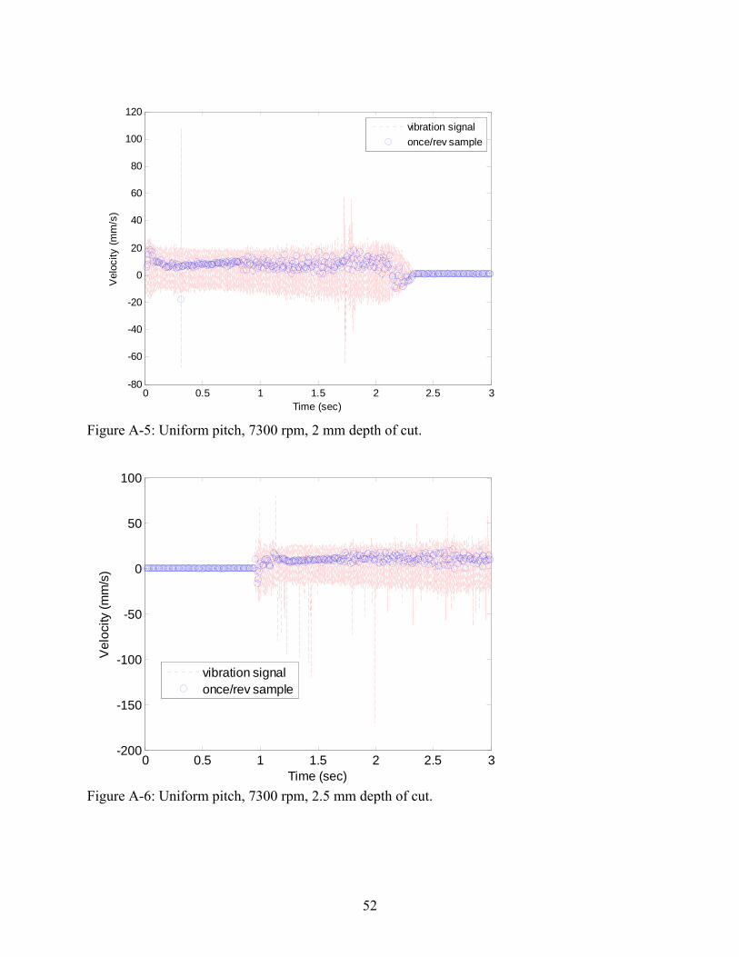
A-5: Uniform pitch, 7300 rpm, 2 mm depth of cut. ......................................................................52
A-6: Uniform pitch, 7300 rpm, 2.5 mm depth of cut. ...................................................................52
A-7: Uniform pitch, 7300 rpm, 3 mm depth of cut. ......................................................................53

9
A-8: Uniform pitch, 7300 rpm, 3.5 mm depth of cut. ...................................................................53
A-9: Uniform pitch, 7300 rpm, 4 mm depth of cut. ......................................................................54
A-10: Uniform pitch, 11,000 rpm, 5.5 mm depth of cut. ..............................................................54
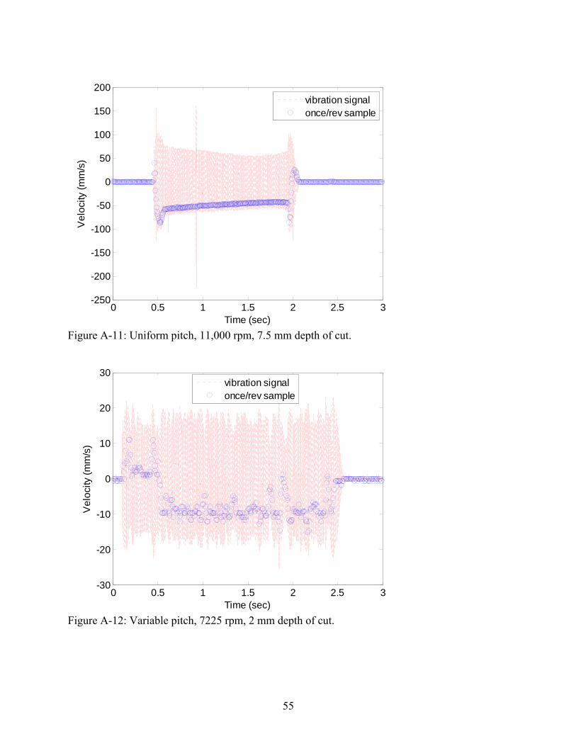
A-11: Uniform pitch, 11,000 rpm, 7.5 mm depth of cut. ..............................................................55
A-12: Variable pitch, 7225 rpm, 2 mm depth of cut. ....................................................................55
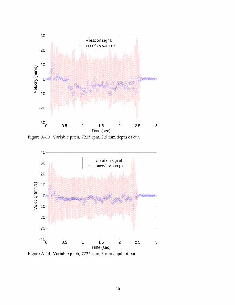
A-13: Variable pitch, 7225 rpm, 2.5 mm depth of cut. .................................................................56
A-14: Variable pitch, 7225 rpm, 3 mm depth of cut. ....................................................................56
A-15: Variable pitch, 7225 rpm, 3.5 mm depth of cut. .................................................................57
A-16: Variable pitch, 7225 rpm, 4 mm depth of cut. ....................................................................57
A-17: Variable pitch, 7225 rpm, 4.5 mm depth of cut. .................................................................58
A-18: Variable pitch, 7225 rpm, 5 mm depth of cut. ....................................................................58
A-19: Variable pitch, 7300 rpm, 3 mm depth of cut. ....................................................................59
A-20: Variable pitch, 7300 rpm, 3.5 mm depth of cut. .................................................................59
A-21: Variable pitch, 7300 rpm, 4 mm depth of cut. ....................................................................60
A-22: Variable pitch, 7300 rpm, 4.5 mm depth of cut. .................................................................60
A-23: Variable pitch, 11,000 rpm, 5.5 mm depth of cut. ..............................................................61
A-24: Variable pitch, 11,000 rpm, 7.5 mm depth of cut. ..............................................................61

10
Abstract of Thesis Presented to the Graduate School of the University of Florida in Partial Fulfillment of the
Requirements for the Degree of Master of Science
CUTTING PERFORMANCE AND STABILITY OF HELICAL ENDMILLS WITH
VARIABLE PITCH
By
Kevin Brady Powell
May 2008
Chair: Tony L. Schmitz Major: Mechanical Engineering
Advancements in machining technology have enabled increasingly aggressive machining
operations with the goal of increasing material removal rate (MRR) to enhance productivity and
reduce production cost. In a high speed machining (HSM) operation, spindle speeds are
increased to a range which is greater than those traditionally used for a given material in order to
achieve an increase in MRR. One mechanism which limits the achievable MRR in machining
operations is self-excited vibrations of the cutting tool, known as chatter. Chatter is caused by
variations in the instantaneous chip thickness caused when the vibration of the tooth currently
engaged in the cut is out of phase with the vibration of the previous tooth. The boundary between
stable and unstable combinations of spindle speed and axial depth of cut for a unique machining
setup are a function of the workpiece material, tool and workpiece dynamics, and the selected
cutting parameters. In some cases, nontraditional tool geometries (such as serrated tool flutes or
variable tooth pitch) can be used to interrupt the feedback mechanism for the tool vibrations, thus
altering the stability of the operation.
In this study a simulation was developed with the goal of predicting the milling stability
for helical endmills, including cutters with variable tooth pitch. This simulation can be used in
11
the future to develop new cutting tools with the goal of maximizing the material removal rate
within a desired spindle speed range. A new way to represent machining stability using the force
output of the time domain simulation was also described. By generating a contour plot of the
peak-to-peak force for a range of axial depths of cut and spindle speeds, a diagram of stable and
unstable combinations of axial depth of cut and spindle speed can be developed. This new
diagram can be directly compared to traditional stability lobe diagrams.
The simulation was validated using equal pitch (traditional) and variable pitch endmills.
The first task was to determine if cutting force coefficients (for a force model) obtained from the
traditional cutting tool could be used to accurately predict the cutting forces of the variable pitch
cutting tool. After successful validation of this step, stability predictions for each of the endmill
geometries were completed using the simulation. Through a series of cutting tests, the stability
limit for each tool was determined at selected spindle speeds. The predicted stability limit
showed good agreement with the experimental limit determined from the cutting tests for both
the traditional and the pitch geometries. The simulation can therefore be used for process
optimization for a given tool or at the design stage to predict the performance of new geometries.

12
CHAPTER 1 INTRODUCTION
The goal of high speed machining is to achieve a significant increase in material removal
rate (MRR), which can significantly reduce production cost and increase production rate. A high
MRR is achieved by the combination of increased axial depth of cut and higher spindle speed.
Advancements in spindle technology have enabled greater spindle speeds while maintaining the
necessary power to perform aggressive cutting operations. In high speed machining operations,
the mechanism that limits the achievable MRR is the process instability known as chatter.
Chatter is a self-excited vibration caused by variations in instantaneous chip thickness (the
thickness of the material being removed by a tooth at a point in time). When a flexible tool
engages a workpiece, the tool begins to vibrate; these vibrations are cut into the new surface,
leaving a wavy surface. As the next tooth cuts through the workpiece, the wavy surface creates
variations in the instantaneous chip thickness. This, in turn, modulates the force on the cutting
tool, creating a feedback mechanism for the tool vibrations. If the current vibration of the cutting
tool is in-phase with the wavy surface left by the previous tooth, the instantaneous chip thickness
remains nearly constant and vibrations tend to decay resulting in stable cutting conditions. If the
vibration of the cutting tool is out-of-phase with the previous surface, the variations in the
instantaneous chip thickness can lead to unstable cutting conditions or chatter. The force and
vibration levels during chatter are large and can damage the workpiece and/or tool. In some
cases, nontraditional tool geometries (such as serrated tool flutes or variable tooth pitch) can be
used to interrupt the feedback mechanism for the tool vibrations, thus altering the stability of the
operation. It has also been shown that endmills with variable tooth pitch can reduce the location
error of the finished surface [1].

13
The boundary between stable and unstable combinations of spindle speed and axial depth
of cut for a unique machining setup are a function of the workpiece material, tool and workpiece
dynamics, and the selected cutting parameters. The ability to predict the combinations of spindle
speed and axial depth of cut which can provide the greatest MRR can eliminate the need for
expensive and time consuming cutting tests.
The goal of this project is to develop and validate a numerical algorithm that can be used to
predict the stability of variable pitch helical endmills for the purpose of tool design. A key
component of stability prediction is the relationship between the cutting force and the uncut chip
area, which can be linked by cutting force coefficients. The first objective of the project is to
verify that previously documented cutting force coefficients of traditional endmills could be used
to predict the cutting forces of variable pitch endmills, therefore eliminating the need for cutting
force measurements in future predictions. Once the cutting force coefficients of the variable pitch
endmill are identified, a time-domain simulation is used to develop a stability lobe diagram, or
map of stable and unstable spindle speed-axial depth of cut combinations, which can be used at
the cutter design stage to select appropriate tooth spacing values for improved process
performance.
14
CHAPTER 2 LITERATURE REVIEW
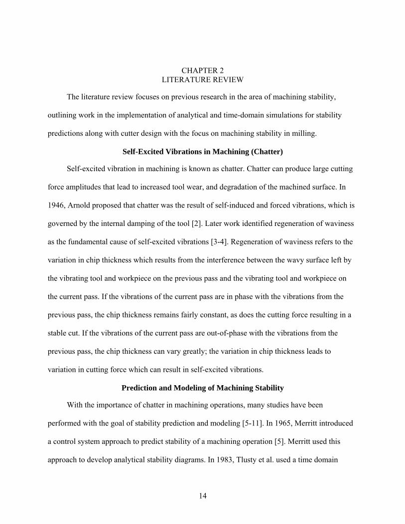
The literature review focuses on previous research in the area of machining stability,
outlining work in the implementation of analytical and time-domain simulations for stability
predictions along with cutter design with the focus on machining stability in milling.
Self-Excited Vibrations in Machining (Chatter)
Self-excited vibration in machining is known as chatter. Chatter can produce large cutting
force amplitudes that lead to increased tool wear, and degradation of the machined surface. In
1946, Arnold proposed that chatter was the result of self-induced and forced vibrations, which is
governed by the internal damping of the tool [2]. Later work identified regeneration of waviness
as the fundamental cause of self-excited vibrations [3-4]. Regeneration of waviness refers to the
variation in chip thickness which results from the interference between the wavy surface left by
the vibrating tool and workpiece on the previous pass and the vibrating tool and workpiece on
the current pass. If the vibrations of the current pass are in phase with the vibrations from the
previous pass, the chip thickness remains fairly constant, as does the cutting force resulting in a
stable cut. If the vibrations of the current pass are out-of-phase with the vibrations from the
previous pass, the chip thickness can vary greatly; the variation in chip thickness leads to
variation in cutting force which can result in self-excited vibrations.
Prediction and Modeling of Machining Stability
With the importance of chatter in machining operations, many studies have been
performed with the goal of stability prediction and modeling [5-11]. In 1965, Merritt introduced
a control system approach to predict stability of a machining operation [5]. Merritt used this
approach to develop analytical stability diagrams. In 1983, Tlusty et al. used a time domain
15
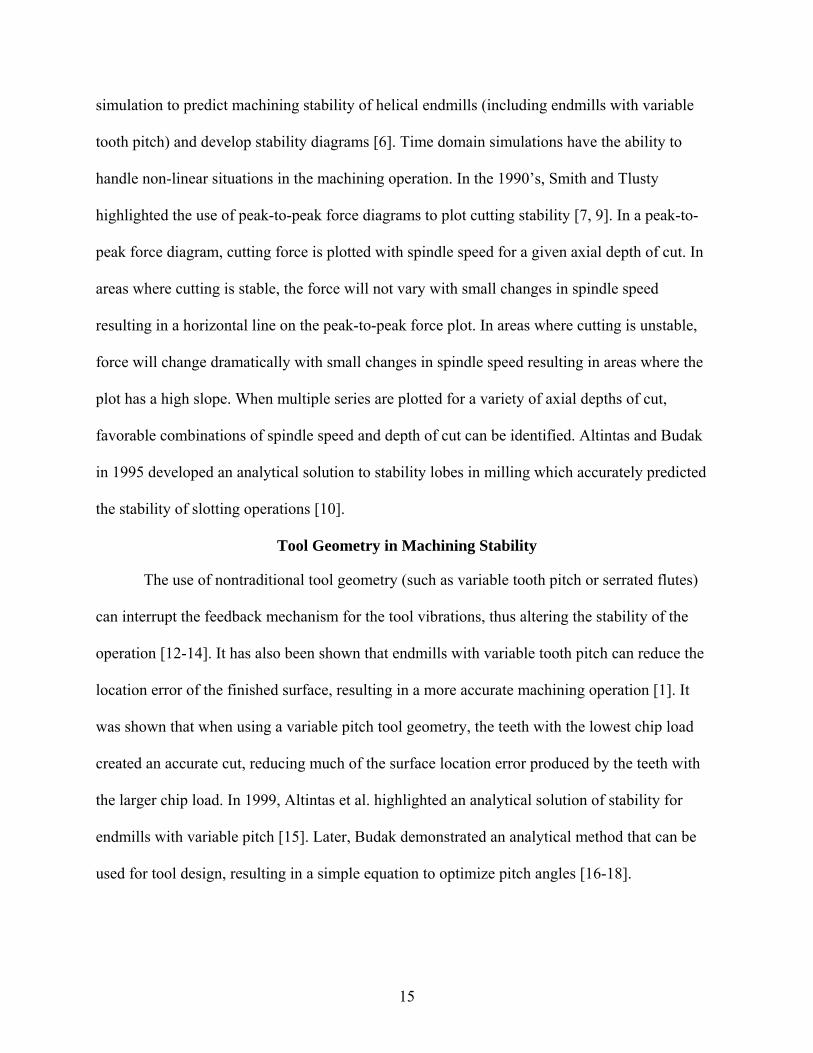
simulation to predict machining stability of helical endmills (including endmills with variable
tooth pitch) and develop stability diagrams [6]. Time domain simulations have the ability to
handle non-linear situations in the machining operation. In the 1990’s, Smith and Tlusty
highlighted the use of peak-to-peak force diagrams to plot cutting stability [7, 9]. In a peak-to-
peak force diagram, cutting force is plotted with spindle speed for a given axial depth of cut. In
areas where cutting is stable, the force will not vary with small changes in spindle speed
resulting in a horizontal line on the peak-to-peak force plot. In areas where cutting is unstable,
force will change dramatically with small changes in spindle speed resulting in areas where the
plot has a high slope. When multiple series are plotted for a variety of axial depths of cut,
favorable combinations of spindle speed and depth of cut can be identified. Altintas and Budak
in 1995 developed an analytical solution to stability lobes in milling which accurately predicted
the stability of slotting operations [10].
Tool Geometry in Machining Stability
The use of nontraditional tool geometry (such as variable tooth pitch or serrated flutes)
can interrupt the feedback mechanism for the tool vibrations, thus altering the stability of the
operation [12-14]. It has also been shown that endmills with variable tooth pitch can reduce the
location error of the finished surface, resulting in a more accurate machining operation [1]. It
was shown that when using a variable pitch tool geometry, the teeth with the lowest chip load
created an accurate cut, reducing much of the surface location error produced by the teeth with
the larger chip load. In 1999, Altintas et al. highlighted an analytical solution of stability for
endmills with variable pitch [15]. Later, Budak demonstrated an analytical method that can be
used for tool design, resulting in a simple equation to optimize pitch angles [16-18].
16
CHAPTER 3 CUTTING FORCE MODEL
Development
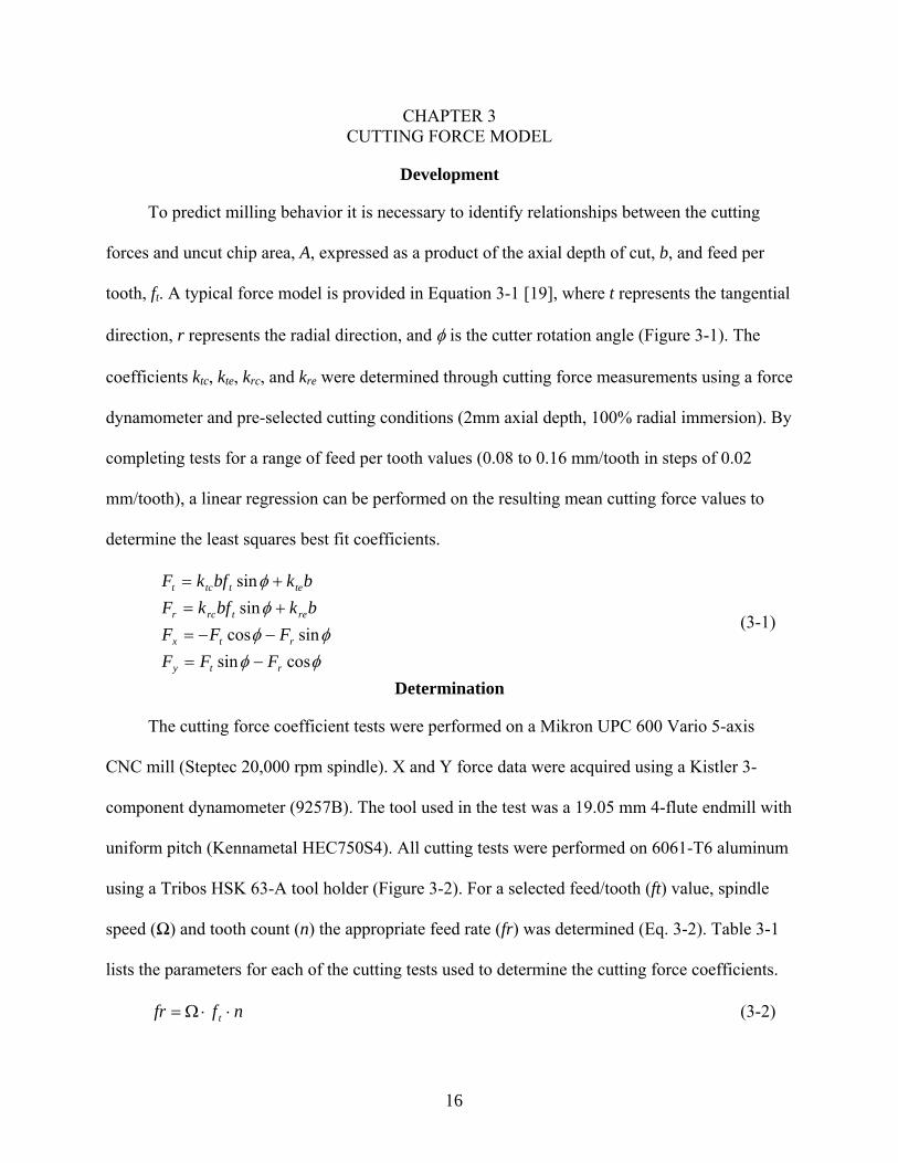
To predict milling behavior it is necessary to identify relationships between the cutting
forces and uncut chip area, A, expressed as a product of the axial depth of cut, b, and feed per
tooth, ft. A typical force model is provided in Equation 3-1 [19], where t represents the tangential
direction, r represents the radial direction, and φ is the cutter rotation angle (Figure 3-1). The
coefficients ktc, kte, krc, and kre were determined through cutting force measurements using a force
dynamometer and pre-selected cutting conditions (2mm axial depth, 100% radial immersion). By
completing tests for a range of feed per tooth values (0.08 to 0.16 mm/tooth in steps of 0.02
mm/tooth), a linear regression can be performed on the resulting mean cutting force values to
determine the least squares best fit coefficients.
φφφφ
φφ
cossinsincos
sinsin
rty
rtx
retrcr
tettct
FFFFFF
bkbfkFbkbfkF
−=−−=+=+=
(3-1)
Determination
The cutting force coefficient tests were performed on a Mikron UPC 600 Vario 5-axis
CNC mill (Steptec 20,000 rpm spindle). X and Y force data were acquired using a Kistler 3-
component dynamometer (9257B). The tool used in the test was a 19.05 mm 4-flute endmill with
uniform pitch (Kennametal HEC750S4). All cutting tests were performed on 6061-T6 aluminum
using a Tribos HSK 63-A tool holder (Figure 3-2). For a selected feed/tooth (ft) value, spindle
speed (Ω) and tooth count (n) the appropriate feed rate (fr) was determined (Eq. 3-2). Table 3-1
lists the parameters for each of the cutting tests used to determine the cutting force coefficients.
nffr t ⋅⋅Ω= (3-2)
17
Table 3-2 shows the cutting force coefficient results. The values were obtained from the
linear regression through the mean cutting forces (see Figure 3-3 through Figure 3-6) for each of
the four spindle speeds. Each of the points on the mean force versus feed per tooth plot (see
Figure 3-3 through Figure 3-6) represents the mean cutting force for a particular feed rate. The
results show a decrease in the tangential cutting force coefficient as the spindle speed is
increased; this trend matches previous experimental results. It is theorized that combination of
increased strain rate and thermal softening of the workpiece at higher cutting speeds can affect
the force required to cut the material, resulting in a change in the cutting force coefficients with
spindle speed [20].
Figure 3-1: Cutting force model.
ft fr
φ
x
y Fr
Ft
Fx
Fy

18
Figure 3-2: Cutting force coefficient test setup.
0.8 0.9 1 1.1 1.2 1.3 1.4 1.5 1.6 1.7
x 10-4
-180
-160
-140
-120
-100
F X (N)
ft (m/tooth)
0.8 0.9 1 1.1 1.2 1.3 1.4 1.5 1.6 1.7
x 10-4
150
200
250
300
350
F Y (N
)
ft (m/tooth)
Figure 3-3: Mean cutting force versus feed rate (2000 rpm, ADOC = 2 mm)
+Z
+X
+Y
Tribos HSK 63-A Holder
Kistler dynamometer
Kennametal HEC750S4 Endmill

19
0.8 0.9 1 1.1 1.2 1.3 1.4 1.5 1.6 1.7
x 10-4
-100
-90
-80
-70F X (N
)
ft (m/tooth)
0.8 0.9 1 1.1 1.2 1.3 1.4 1.5 1.6 1.7
x 10-4
100
150
200
250
300
F Y (N
)
ft (m/tooth)
Figure 3-4: Mean cutting force versus feed rate (6000 rpm, ADOC = 2 mm)
0.8 0.9 1 1.1 1.2 1.3 1.4 1.5 1.6 1.7
x 10-4
-80
-70
-60
-50
F X (N)
ft (m/tooth)
0.8 0.9 1 1.1 1.2 1.3 1.4 1.5 1.6 1.7
x 10-4
100
150
200
250
F Y (N
)
ft (m/tooth)
Figure 3-5: Mean cutting force versus feed rate (10,000 rpm, ADOC = 2 mm)

20
0.8 0.9 1 1.1 1.2 1.3 1.4 1.5 1.6 1.7
x 10-4
-70
-60
-50
-40F X (N
)
ft (m/tooth)
0.8 0.9 1 1.1 1.2 1.3 1.4 1.5 1.6 1.7
x 10-4
100
150
200
250
F Y (N
)
ft (m/tooth)
Figure 3-6: Mean cutting force versus feed rate (15,000 rpm, ADOC = 2 mm)
Table 3-1: Cutting tests to determine cutting force coefficients.
Setup Cut Spindle Speed (rpm) Axial Depth (mm)
Radial Immersion
Feed/Tooth (mm)
Feed Rate (mm/min)
1 2000 2 100% 0.08 640 2 2000 2 100% 0.10 800 3 2000 2 100% 0.12 960 4 2000 2 100% 0.14 1120
1 5 2000 2 100% 0.16 1280 1 6000 2 100% 0.08 1920 2 6000 2 100% 0.10 2400 3 6000 2 100% 0.12 2880 4 6000 2 100% 0.14 3360
2 5 6000 2 100% 0.16 3840 1 10000 2 100% 0.08 3200 2 10000 2 100% 0.10 4000 3 10000 2 100% 0.12 4800 4 10000 2 100% 0.14 5600
3 5 10000 2 100% 0.16 6400 1 15000 2 100% 0.08 4800 2 15000 2 100% 0.10 6000 3 15000 2 100% 0.12 7200 4 15000 2 100% 0.14 8400
4 5 15000 2 100% 0.16 9600

21
Table 3-2: Cutting force coefficients (Kennametal HEC750S4) rpm 2000 6000 10,000 15,000 Ktc (N/m2) 7.58x10⁸ 6.41x10⁸ 6.13x10⁸ 5.94x10⁸ Kte (N/m) 2.61x10⁴ 1.78x10⁴ 1.41x10⁴ 1.44x10⁴ Krc (N/m2) 3.50x10⁸ 1.47x10⁸ 1.11x10⁸ 8.99x10⁷ Kre (N/m) 2.09x10⁴ 1.87x10⁴ 1.47x10⁴ 1.39x10⁴

22
CHAPTER 4 TIME DOMAIN SIMULATION
Description
A time domain simulation was used to determine the cutting forces between the tool and
workpiece (the simulation is provided in Appendix B). The milling simulation implemented in
this project is time-marching, using Euler integration while moving through time in discrete
steps. At each step the cutter is rotated by a small angle, φd and it is then determined which teeth
are engaged in the cut (the tooth is within the angles prescribed by the radial immersion). If the
tooth is engaged in the cut, the instantaneous chip thickness, h, is determined (based on the cut
geometry and current system vibrations). If h has a value greater than zero, the cutting force is
computed using the force model described in equation (3-1). If h has a value less than or equal to
zero, the tool is said to have moved out of the cut, and the cutting forces are set to zero.
The cutting force simulation requires the input of modal parameters (a description of the
system dynamics), the tool geometry, and machining specifications. The modal parameters
include the stiffness, damping ratio and natural frequency for each tool mode in the x and y-
directions. The tool geometry includes the number of teeth, helix angle, tooth-to-tooth angle,
cutter diameter and the flute-to-flute runout. The machining specifications needed are the starting
and exit angles (a function of cut and radial immersion), spindle speed, axial depth of cut and
feed per tooth. The feed per tooth of a variable pitch tool, ft,unequal, varies from tooth to tooth as a
function of the tooth-to-tooth angle, toothtotooth −−θ (deg), the mean feed per tooth, meantf , (m/tooth),
and the number of teeth, m. The feed per tooth of a particular tooth is described by Equation 4-1.
°
°−− ⋅⋅
=360
,,
mff toothtotoothmeant
unequalt
θ (4-1)

23
Verification
The initial goal of the time domain simulation was to determine if cutting force
coefficients from a tool with uniform pitch could be used to predict cutting forces of a tool with
variable pitch. Figure 4-1 shows the x and y-direction forces measured during a 25% radial
immersion cut in 6160-T6 aluminum using a tool with variable pitch, along with the time domain
simulation results with and without runout. It can be seen in Figure 4-1 that the model accurately
depicts the cutting forces of the cutter with variable pitch using the cutting force coefficients
from the uniform pitch cutter (Table 3-2). The time domain simulation accurately captured the
two different dwell times (the time between one tooth leaving the cut and the next tooth entering
the cut) corresponding to the two flute separation angles. Flute-to-flute runout was added to the
time domain simulation by fitting the simulation results to the measured results. Flute-to-flute
runout accounts for the small variations in tooth radius commonly seen in multi-flute endmills.
The flute-to-flute runout for the tool with variable pitch was between 0 and -15 micrometers.
Since cutting forces for a tool with variable pitch can be accurately predicted using the
cutting force coefficients from a tool with uniform pitch, the cutting force coefficients shown in
Table 3-2 can be used for future predictions. Therefore, extensive cutting tests to determine the
cutting force coefficients for a tool with variable pitch in various materials would not need to be
performed provided that the cutting edge geometry is similar to the geometry used in this study.

24
0.02 0.03 0.04 0.05 0.06 0.07 0.08 0.09 0.1 0.11-50
0
50
100
150
F x (N)
Model w/ RunoutModel w/o RunoutMeasured
0.02 0.03 0.04 0.05 0.06 0.07 0.08 0.09 0.1 0.11-100
0
100
200
300
Time (s)
F y (N)
Figure 4-1 Time domain simulation results for an endmill with variable pitch at 25% radial immersion.

25
CHAPTER 5 PEAK-TO-PEAK STABILITY LOBE IMPLEMENTATION
The chip thickness is a function of the cutter vibrations (projected into the normal of the
cut surface at that instance in time), flute-to-flute runout, and the surface left by the previous
tooth (Figure 5-1).
Figure 5-1: Chip thickness variation due to cutter vibrations.
Since the tool and workpiece are not rigid, they vibrate as the flutes of the tool move
through the workpiece. The vibration results in the tooth leaving a wavy surface behind on the
workpiece. The variations in the instantaneous chip thickness result from the phasing between
the surface left by the previous tooth and the current tooth. The magnitude and phase of the
vibration are governed by the tool and workpiece dynamics. Depending on the phasing, the
forces can grow (unstable cutting, chatter, see Figure 5-2), or remain uniform (stable cutting, see
Figure 5-3).
To help visualize the relationship between cutting stability, axial depth of cut and spindle
speed, analytical stability lobes were developed [6, 10]. Stability lobes are a function of the
process parameters, tool geometry, cutting parameters and system dynamics. These analytical
stability lobes assume the tooth-to-tooth angle is constant. The time domain simulation was used
to determine stability of a tool with variable pitch.
26
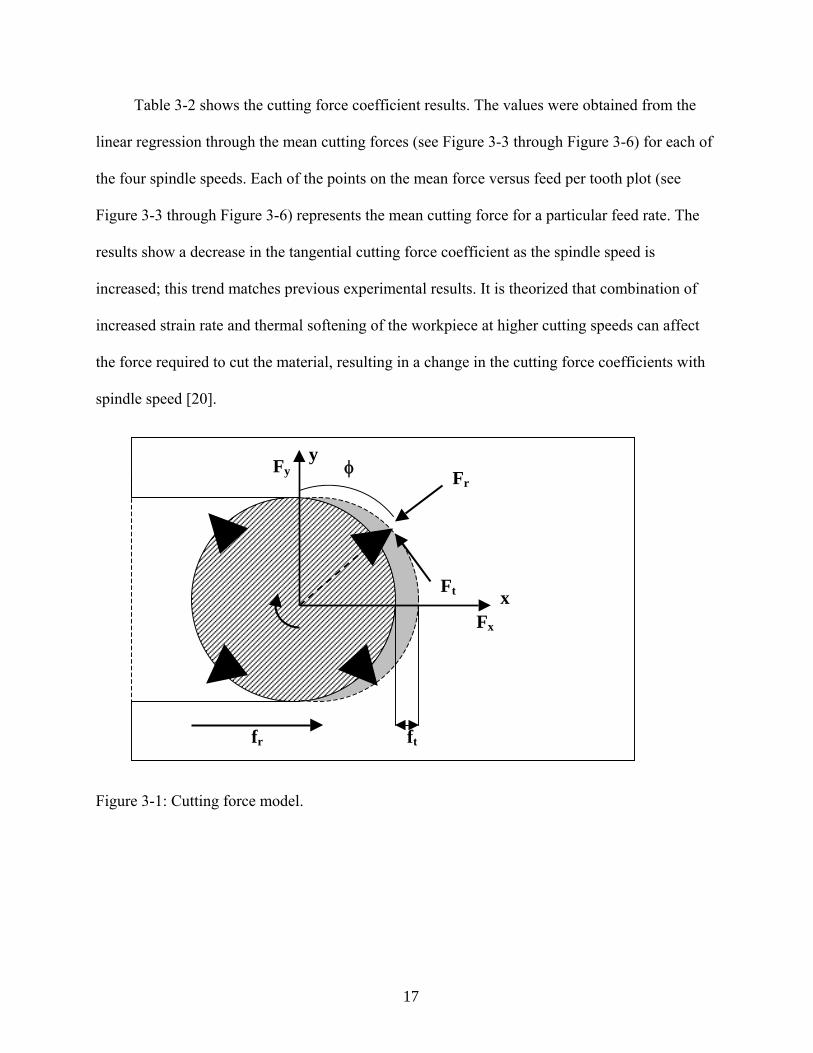
The time domain simulation outlined in the previous chapter was used to predict cutting
forces for a specified spindle speed and axial depth of cut. Stability was determined by plotting
the peak-to-peak (PTP) force values for a range of spindle speed and axial depth of cut
combinations [7, 9]. Figure 5-4 is an example of a PTP force plot ranging from 6000 rpm to
18000 rpm and 1 mm to 10 mm axial depth of cut for a tool with uniform pitch. On the PTP
force plot, each line represents a different axial depth of cut, b (in increments of 0.5mm). When a
cut is in a stable region, the PTP force will not vary with small changes in spindle speed (see
Figure 5-4, zero slope areas). When a cut is in an unstable region, the PTP force will change
dramatically with small changes in spindle speed (see Figure 5-4, high slope areas outlined with
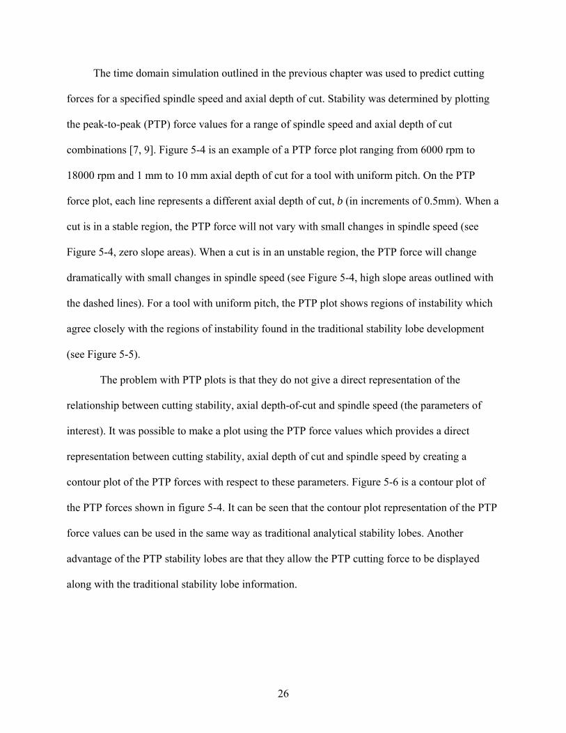
the dashed lines). For a tool with uniform pitch, the PTP plot shows regions of instability which
agree closely with the regions of instability found in the traditional stability lobe development
(see Figure 5-5).
The problem with PTP plots is that they do not give a direct representation of the
relationship between cutting stability, axial depth-of-cut and spindle speed (the parameters of
interest). It was possible to make a plot using the PTP force values which provides a direct
representation between cutting stability, axial depth of cut and spindle speed by creating a
contour plot of the PTP forces with respect to these parameters. Figure 5-6 is a contour plot of
the PTP forces shown in figure 5-4. It can be seen that the contour plot representation of the PTP
force values can be used in the same way as traditional analytical stability lobes. Another
advantage of the PTP stability lobes are that they allow the PTP cutting force to be displayed
along with the traditional stability lobe information.

27
0 0.05 0.1 0.15 0.2 0.25 0.3 0.350
50
100
150
200
250
300
350
400
450
500F x (N
)
Time (s)
Figure 5-2: Force versus time for a tool with uniform pitch at 7200 rpm and a 4 mm axial depth-of-cut (unstable cutting, chatter).
0 0.05 0.1 0.15 0.2 0.25 0.3 0.350
50
100
150
200
250
300
350
400
450
500
F x (N)
Time (s)
Figure 5-3: Force versus time for a tool with variable pitch at 7200 rpm and a 4 mm axial depth-of-cut (stable cutting).
28
0.6 0.8 1 1.2 1.4 1.6 1.8
x 104
0
500
1000
1500
2000
2500
Spindle speed (rpm)
PTP
Fy (N
)
Figure 5-4: Peak-to-peak force plot for a tool with uniform pitch.
0.6 0.8 1 1.2 1.4 1.6 1.8
x 104
0
1
2
3
4
5
6
7
8
9
10
b lim (m
m)
Spindle Speed (rpm)
Figure 5-5: Analytical stability lobes [10].
b=10
Stable
Unstable
b=1
Unstable
Stable

29
89
146
203
260
317
374
431
488
545
602
659
Spindle Speed (rpm)
Axi
al D
epth
(m)
0.6 0.8 1 1.2 1.4 1.6 1.8
x 104
1
2
3
4
5
6
7
8
9
10x 10-3
PTP
Forcey (N)
Figure 5-6: Peak-to-peak stability lobes (uniform pitch).

30
CHAPTER 6 PEAK-TO-PEAK STABILITY LOBE VERIFICATION
Uniform and Variable Pitch Peak-to-Peak Stability Lobe Comparison
The PTP force and stability lobe plots were used to compare a tool with uniform pitch to
a tool with variable pitch to determine if any gains in stability could be achieved. Both tools have
the same cutting geometry except for the tooth-to-tooth angle. The tooth-to-tooth angle for the
endmill with uniform pitch is 90o between all four teeth (see Figure 6-1 A). The tooth-to-tooth
angles for the endmill with variable pitch were 83o and 97o (see Figure 6-1 B). Both tools were
used in the same tool-holder with the same insertion length so that the dynamic responses were
the same.
Figure 6-1: Endmill geometry. A) Uniform pitch (Kennametal HEC750S4). B) Variable pitch.
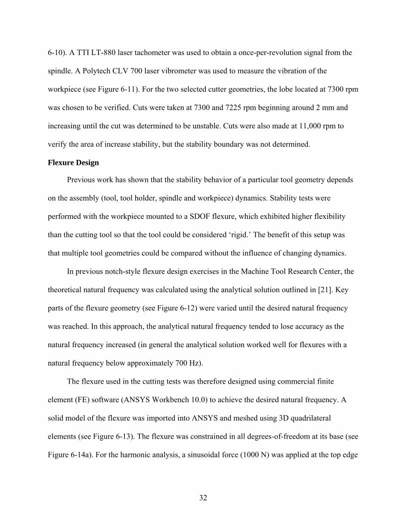
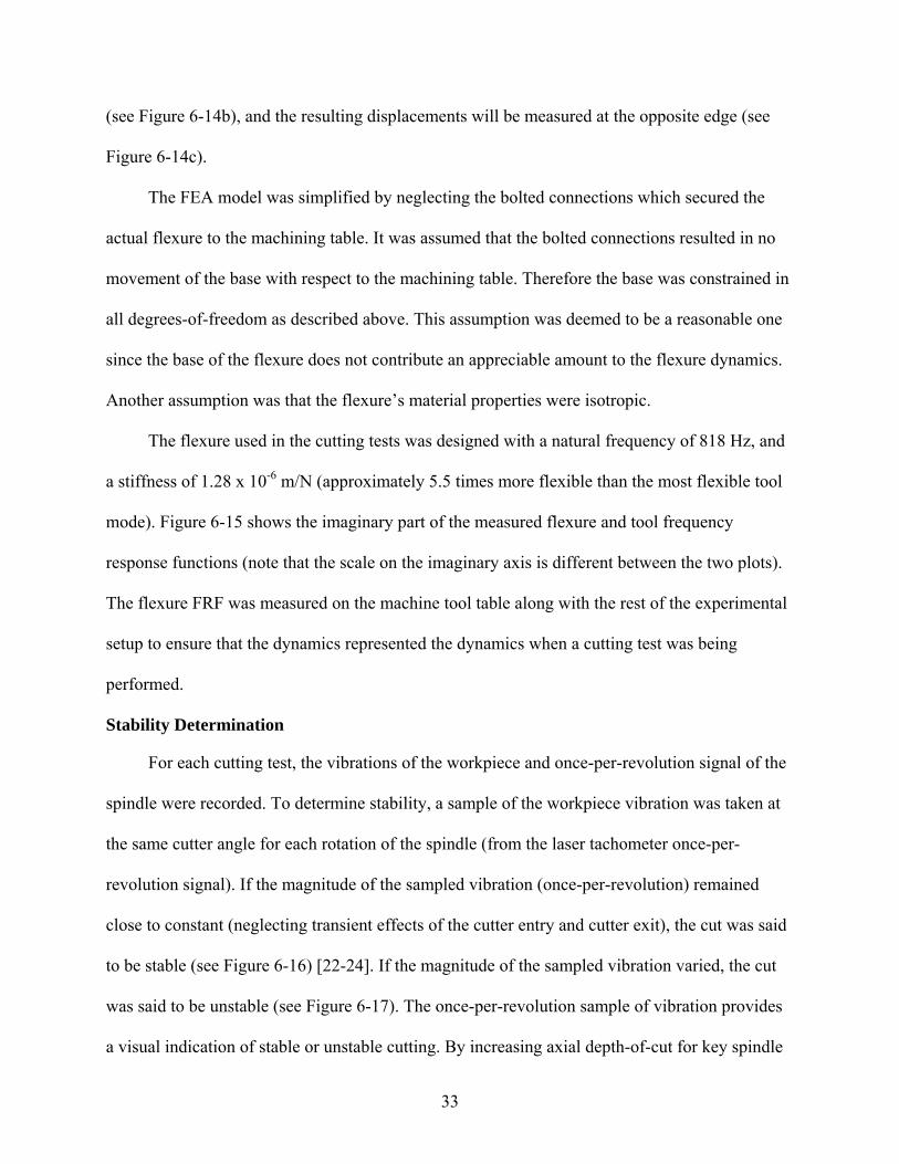
The time domain simulation was performed for each tool (the only change was the tooth-
to-tooth angles), using a 6000 rpm to 12000 rpm spindle speed range and a 1 mm to 10 mm axial
depth of cut range, for a 50% radial immersion up-milling operation (see Figure 6-2 through
Figure 6-5). The PTP force and stability lobe plots for each tool show that near 7300 rpm, the
A B

31
variable pitch tool should perform stable cutting at greater axial depths of cut than the uniform
pitch tool.
Figure 6-6 and 6-7 focus on the lobe near 7300 rpm. It can be seen that the PTP force and
stability lobe plots predict that the boundary of instability occurs at a 3.0 mm axial depth of cut
for a tool with uniform pitch and a spindle speed of 7300 rpm. The PTP force and stability lobe
predictions closely match the stability lobe prediction from [10] (as seen in Figure 5-5). The PTP
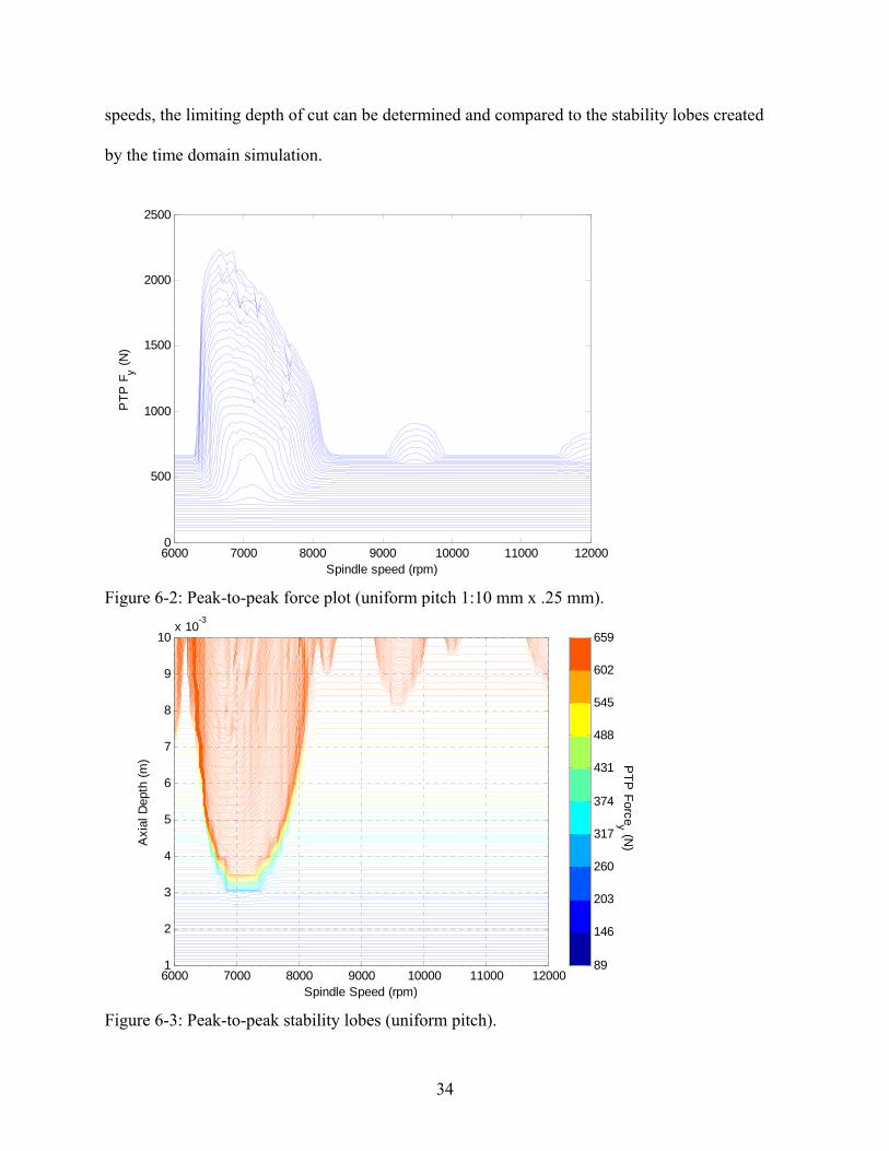
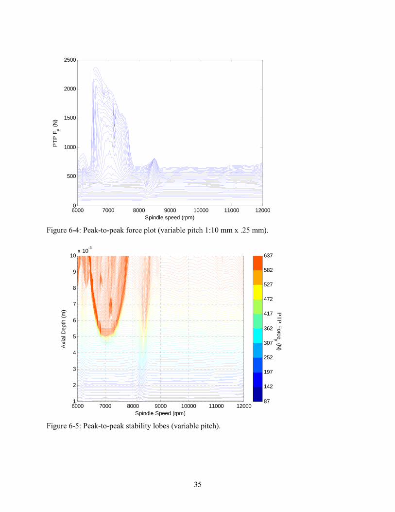
force and stability lobe predictions were then performed for a tool with variable pitch (see Figure
6-1 B), all other process and cutting parameters were unchanged. Figure 6-8 and 6-9 focus on the
same lobe as Figure 6-6 and 6-7 for the tool with variable pitch. The PTP force and stability lobe
plots for the tool with variable pitch show that instability occurs around 4.5 mm axial depth of
cut for a spindle speed of 7300 rpm. The PTP force and stability lobe plots indicate that for a
given set of system dynamics, cutting parameters and spindle speed, the tool described in Figure
6-1 B could achieve a higher material removal rate than the tool described in Figure 6-1 A, while
maintaining stable cutting conditions.
The next step was verify the PTP force plots by performing a series of cutting tests for
different axial depths of cut and spindle speeds. The stability of each cut was determined and the
results were compared to the predictions made by the PTP force plots. The bulk of the
experimental cuts were performed around 7300 rpm to capture the difference in the stability
boundary between the two different tool geometries.
Experimental Setup and Procedure
Cutting Tests
Cutting tests were performed on a Mikron UPC 600 Vario 5-axis CNC mill (Steptec
20,000 rpm spindle). A 6061-T6 aluminum workpiece was mounted on a single degree-of-
freedom (SDOF) notch style flexure which was, in turn, mounted to the machining table (Figure
32
6-10). A TTI LT-880 laser tachometer was used to obtain a once-per-revolution signal from the
spindle. A Polytech CLV 700 laser vibrometer was used to measure the vibration of the
workpiece (see Figure 6-11). For the two selected cutter geometries, the lobe located at 7300 rpm
was chosen to be verified. Cuts were taken at 7300 and 7225 rpm beginning around 2 mm and
increasing until the cut was determined to be unstable. Cuts were also made at 11,000 rpm to
verify the area of increase stability, but the stability boundary was not determined.
Flexure Design
Previous work has shown that the stability behavior of a particular tool geometry depends
on the assembly (tool, tool holder, spindle and workpiece) dynamics. Stability tests were
performed with the workpiece mounted to a SDOF flexure, which exhibited higher flexibility
than the cutting tool so that the tool could be considered ‘rigid.’ The benefit of this setup was
that multiple tool geometries could be compared without the influence of changing dynamics.
In previous notch-style flexure design exercises in the Machine Tool Research Center, the
theoretical natural frequency was calculated using the analytical solution outlined in [21]. Key
parts of the flexure geometry (see Figure 6-12) were varied until the desired natural frequency
was reached. In this approach, the analytical natural frequency tended to lose accuracy as the
natural frequency increased (in general the analytical solution worked well for flexures with a
natural frequency below approximately 700 Hz).
The flexure used in the cutting tests was therefore designed using commercial finite
element (FE) software (ANSYS Workbench 10.0) to achieve the desired natural frequency. A
solid model of the flexure was imported into ANSYS and meshed using 3D quadrilateral
elements (see Figure 6-13). The flexure was constrained in all degrees-of-freedom at its base (see
Figure 6-14a). For the harmonic analysis, a sinusoidal force (1000 N) was applied at the top edge
33
(see Figure 6-14b), and the resulting displacements will be measured at the opposite edge (see
Figure 6-14c).
The FEA model was simplified by neglecting the bolted connections which secured the
actual flexure to the machining table. It was assumed that the bolted connections resulted in no
movement of the base with respect to the machining table. Therefore the base was constrained in
all degrees-of-freedom as described above. This assumption was deemed to be a reasonable one
since the base of the flexure does not contribute an appreciable amount to the flexure dynamics.
Another assumption was that the flexure’s material properties were isotropic.
The flexure used in the cutting tests was designed with a natural frequency of 818 Hz, and
a stiffness of 1.28 x 10⁻⁶ m/N (approximately 5.5 times more flexible than the most flexible tool
mode). Figure 6-15 shows the imaginary part of the measured flexure and tool frequency
response functions (note that the scale on the imaginary axis is different between the two plots).
The flexure FRF was measured on the machine tool table along with the rest of the experimental
setup to ensure that the dynamics represented the dynamics when a cutting test was being
performed.
Stability Determination
For each cutting test, the vibrations of the workpiece and once-per-revolution signal of the
spindle were recorded. To determine stability, a sample of the workpiece vibration was taken at
the same cutter angle for each rotation of the spindle (from the laser tachometer once-per-
revolution signal). If the magnitude of the sampled vibration (once-per-revolution) remained
close to constant (neglecting transient effects of the cutter entry and cutter exit), the cut was said
to be stable (see Figure 6-16) [22-24]. If the magnitude of the sampled vibration varied, the cut
was said to be unstable (see Figure 6-17). The once-per-revolution sample of vibration provides
a visual indication of stable or unstable cutting. By increasing axial depth-of-cut for key spindle
34
speeds, the limiting depth of cut can be determined and compared to the stability lobes created
by the time domain simulation.
6000 7000 8000 9000 10000 11000 120000
500
1000
1500
2000
2500
Spindle speed (rpm)
PTP
Fy (N
)
Figure 6-2: Peak-to-peak force plot (uniform pitch 1:10 mm x .25 mm).
89
146
203
260
317
374
431
488
545
602
659
Spindle Speed (rpm)
Axi
al D
epth
(m)
6000 7000 8000 9000 10000 11000 120001
2
3
4
5
6
7
8
9
10x 10-3
PTP
Forcey (N)
Figure 6-3: Peak-to-peak stability lobes (uniform pitch).
35
6000 7000 8000 9000 10000 11000 120000
500
1000
1500
2000
2500
Spindle speed (rpm)
PTP
Fy (N
)
Figure 6-4: Peak-to-peak force plot (variable pitch 1:10 mm x .25 mm).
87
142
197
252
307
362
417
472
527
582
637
Spindle Speed (rpm)
Axi
al D
epth
(m)
6000 7000 8000 9000 10000 11000 120001
2
3
4
5
6
7
8
9
10x 10-3
PTP
Forcey (N)
Figure 6-5: Peak-to-peak stability lobes (variable pitch).

36
6000 6500 7000 7500 8000 85000
100
200
300
400
500
600
700
800
900
Spindle speed (rpm)
PTP
Fy (N
)
3.5mm
2.5mm2.0mm
3.0mm
4.0mm
Figure 6-6: Peak-to-peak force plot (uniform pitch, 1:10 mm x .25 mm)
89
146
203
260
317
374
431
488
545
602
659
Spindle Speed (rpm)
Axi
al D
epth
(m)
6000 6500 7000 7500 8000 85001
2
3
4
5
6
7
8
9
10x 10
-3
PTP
Forcey (N)
Figure 6-7: Peak-to-peak stability lobes (uniform pitch)

37
6000 6500 7000 7500 8000 85000
100
200
300
400
500
600
700
800
900
Spindle speed (rpm)
PTP
Fy (N
)
3.5mm
2.5mm2.0mm
3.0mm
4.0mm4.5mm
5.0mm
Figure 6-8: Peak-to-peak force plot (variable pitch, 1:10 mm x .25 mm)
87
142
197
252
307
362
417
472
527
582
637
Spindle Speed (rpm)
Axi
al D
epth
(m)
6000 6500 7000 7500 8000 85001
2
3
4
5
6
7
8
9
10x 10-3
PTP
Forcey (N)
Figure 6-9: Peak-to-peak stability lobes (variable pitch).

38
Figure 6-10: Flexure-based cutting test setup.
Figure 6-11: Cutting stability setup.
Laser vibrometer
SDOF flexure
Laser tachometer
Tool holder
Workpiece
Single degree-of-freedom notch-style flexure
Workpiece
Machine tool table
Selected cutting tool

39
Figure 6-12: Key notch-style flexure dimensions (in mm).
Figure 6-13: Flexure model mesh for modal analysis.

40
Figure 6-14: Flexure FEM model. a) Sinusoidal force along the top edge. b) Bottom face
constrained in all DOF’s. c) FRF determined at top edge.
0 500 1000 1500 2000 2500 3000 3500 4000 4500 5000-15
-10
-5
0x 10-7 Flexure
Frequency (Hz)
Imag
inar
y (m
/N)
0 500 1000 1500 2000 2500 3000 3500 4000 4500 5000-3
-2
-1
0
1x 10⁻⁷ Tool-tip
Frequency (Hz)
Imag
inar
y (m
/N)
Figure 6-15: Flexure and tool-tip frequency response functions.
(b) (c)
(a)

41
0 0.5 1 1.5 2 2.5 3-60
-50
-40
-30
-20
-10
0
10
20
30
40
Time (sec)
Vel
ocity
(mm
/s)
vibration signalonce/rev sample
Figure 6-16: Stable cutting vibration (variable pitch, 7300 rpm, 4 mm axial depth-of-cut)
0 0.5 1 1.5 2 2.5 3-150
-100
-50
0
50
100
150
Time (sec)
Vel
ocity
(mm
/s)
vibration signalonce/rev sample
Figure 6-17: Unstable cutting vibration (uniform pitch, 7300 rpm, 4 mm axial depth-of-cut)
42
CHAPTER 7 STABILITY LOBE VERIFICATION RESULTS
For the two selected cutter geometries, the lobe located at 7300 rpm was chosen to be
verified. Cuts were taken at 7300 and 7225 rpm beginning around 2mm and increasing until the
cut was determined to be unstable. Cuts were also made at 11,000 rpm to verify the area of
increase stability, but the stability boundary was not determined. Figure 7-1 and 7-2 show the
results of the experimental cutting tests overlaid with the peak-to-peak cutting force stability
lobes. The O’s on the plot represent cuts that exhibit stable behavior, while the X’s represent cuts
that exhibit unstable behavior.
Figure 7-3 and Figure 7-4 highlight the transition from stable behavior (7300 rpm, 2.5 mm
depth of cut in Figure 7-3) to unstable behavior (7300 rpm, 3.0 mm depth of cut in Figure 7-4) of
the uniform pitch tool. Figure 7-5 and Figure 7-6 highlight the transition from stable behavior
(7300 rpm, 4.0 mm depth of cut in Figure 7-5) to unstable behavior (7300 rpm, 4.5 mm depth of
cut in Figure 7-6) of the variable pitch tool. The results of all the cutting test results performed in
this study can be seen in Appendix A.
The PTP stability lobes provide a good indication of the stable regions for a particular set
of system dynamics and cutting conditions for both tools. Improvements to the PTP stability lobe
accuracy can be made by increasing the number of revolutions calculated and decreasing the
spindle speed and axial depth step size in the time domain simulation at the expense of
computation time.

43
89
146
203
260
317
374
431
488
545
602
659
ooxx
ooxxx
o
o
Spindle Speed (rpm)
Axi
al D
epth
(m)
6000 7000 8000 9000 10000 11000 120001
2
3
4
5
6
7
8
9
10x 10-3
PTP
Forcey (N)
Figure 7-1: Peak-to-peak stability lobes with experimental results (uniform pitch).
87
142
197
252
307
362
417
472
527
582
637
oooooxx
ooox
o
o
Spindle Speed (rpm)
Axi
al D
epth
(m)
6000 7000 8000 9000 10000 11000 120001
2
3
4
5
6
7
8
9
10x 10-3
PTP
Forcey (N)
Figure 7-2: Peak-to-peak stability lobes with experimental results (variable pitch).

44
0 0.5 1 1.5 2 2.5 3-200
-150
-100
-50
0
50
100
Time (sec)
Vel
ocity
(mm
/s)
vibration signalonce/rev sample
Figure 7-3: Uniform pitch, 7300 rpm, 2.5 mm depth of cut (stable).
0 0.5 1 1.5 2 2.5 3-120
-100
-80
-60
-40
-20
0
20
40
Time (sec)
Vel
ocity
(mm
/s)
vibration signalonce/rev sample
Figure 7-4: Uniform pitch, 7300 rpm, 3 mm depth of cut (unstable).

45
0 0.5 1 1.5 2 2.5 3-60
-50
-40
-30
-20
-10
0
10
20
30
40
Time (sec)
Vel
ocity
(mm
/s)
vibration signalonce/rev sample
Figure 7-5: Variable pitch, 7300 rpm, 4 mm depth of cut (stable).
0 0.5 1 1.5 2 2.5 3-150
-100
-50
0
50
100
Time (sec)
Vel
ocity
(mm
/s)
vibration signalonce/rev sample
Figure 7-6: Variable pitch, 7300 rpm, 4.5 mm depth of cut (unstable).
46
CHAPTER 8 CONCLUSION
The goal of this project was to develop a time domain simulation which can be used to
predict the stability behavior of helical endmills with unequal pitch. This simulation can be
implemented for milling process optimization (for a given cutter) or at the design stage when
selecting tooth angles for a particular cutting tool (and associated process dynamics). The
stability of the machining process was expressed using a new representation of the peak-to-peak
force diagram. By generating a contour plot of the peak-to-peak force for a range of axial depths
of cut, a diagram of stable and unstable combinations of axial depth of cut and spindle speed was
developed; this diagram provides the same same information as traditional stability lobe
diagrams, but can be applied to cutters with unequal pitch. The benefit of the new diagram over
peak-to-peak force plots is that the two axes of the contour plot directly correspond to the cutting
parameters used to characterize a milling operation, namely spindle speed and axial depth of cut
(for a preselected radial immersion).
In order to predict cutting forces and, eventually stability behavior, cutting force
coefficients for an appropriate force model are required. The first task was to verify that cutting
force coefficients obtained from tests using equal pitch cutting tools could be used to predict
cutting forces for variable pitch cutters. By measuring the forces exerted on a workpiece during a
variety of cutting operations, the cutting force coefficients were determined. The cutting force
coefficients were obtained for both equal and variable pitch endmills while keeping all other
cutter geometric parameters the same. The cutting force coefficients from the equal pitch endmill
were used later in the project to predict the cutting forces of the variable pitch cutter. The
predicted cutting forces matched the measured cutting forces; therefore, previously documented
cutting force coefficients for traditional cutters can be used in future predictions. This is a
47
necessary step for cutting tool design since it was desired to make process predictions for
arbitrary designs and avoid producing the cutter if unfavorable results were obtained.
Finally, predictions for the variable and equal pitch endmills were made using the
simulation. The predictions were then validated by performing a sequence of cutting tests while
measuring the workpiece deflections. The vibrations measured during each cutting test was used
to determine the stability of the cut. If the vibrations became larger with the passing of time the
cut was said to be unstable. If the vibrations remained constant with time, the cut was said to be
stable. The predicted stability in the critical areas tested for both the traditional geometry endmill
and the variable pitch endmill matched well with the experimental stability test results.
One of the difficulties encountered in this project was a chip evacuation for 100% radial
immersion conditions when using the variable pitch endmill. As seen in Figure 8-1, the problem
occurs between the cutting teeth which have the smaller tooth-to-tooth spacing. Figure 8-2 shows
a closeup of the built-up material. It is observed that after the first chip becomes welded to the
tooth, subsequent chips are welded to the previous chip leaving layered material affixed to the
cutting tooth. The built-up material results in a significant increase in cutting forces since the
there is no longer a sharp tooth to move smoothly through the workpiece material. The increase
in cutting forces can be seen graphically in Figure 8-3 which is a plot of the force values
recorded by the dynamometer during one such incident. The first solution that was attempted
was to add a jet of compressed air, aimed at the base of the cutter. The hope was that the jet of air
would help to evacuate the cut chips before they had the opportunity to become welded to the
tooth surface. Unfortunately, adding the compressed air had little effect on preventing the chips
from becoming welded. The workaround was to limit the radial immersion of the cutting tests to
50%. Reducing the radial immersion provided a more direct path for chip removal and allowed

48
more time for the tooth face to cool while outside the cut. The use of flood coolant may eliminate
this phenomenon, but this potential solution was not explored. This is an important observation
because it may limit the pitch variation which can be reasonably achieved in pitch tuning
exercises for chatter avoidance.
In future work, a variety of unique variable pitch endmills should be tested. In these tests,
the effectiveness of various types of coolant and lubrication on preventing the build up of
material on cutting teeth should be determined. If the addition of flood coolant or other types of
lubrication prove to be ineffective, the limits of tool geometry and variable pitch cutting
parameters should be identified. Also, an error sensitivity analysis should be performed on the
various inputs used by the prediction stability tool to determine the effect of measurement and
tool geometry errors on the accuracy of stability predictions using the peak-to-peak force method
[25].
Figure 8-1: Workpiece chips welded to cutting teeth
49
Figure 8-2: Close up of welded chips
Figure 8-3: Cutting forces during welded chip cut test

50
APPENDIX A ONCE-PER-REVOLUTION PLOTS
0 0.5 1 1.5 2 2.5 3-40
-30
-20
-10
0
10
20
30
40
Time (sec)
Vel
ocity
(mm
/s)
vibration signalonce/rev sample
Figure A-1: Uniform pitch, 7225 rpm, 2 mm depth of cut.
0 0.5 1 1.5 2 2.5 3-50
-40
-30
-20
-10
0
10
20
30
40
50
Time (sec)
Vel
ocity
(mm
/s)
vibration signalonce/rev sample
Figure A-2: Uniform pitch, 7225 rpm, 2.5 mm depth of cut.

51
0 0.5 1 1.5 2 2.5 3-80
-60
-40
-20
0
20
40
60
80
Time (sec)
Vel
ocity
(mm
/s)
vibration signalonce/rev sample
Figure A-3: Uniform pitch, 7225 rpm, 3 mm depth of cut.
0 0.5 1 1.5 2 2.5 3-200
-150
-100
-50
0
50
100
150
200
Time (sec)
Vel
ocity
(mm
/s)
vibration signalonce/rev sample
Figure A-4: Uniform pitch, 7225 rpm, 3.5 mm depth of cut.
52
0 0.5 1 1.5 2 2.5 3-80
-60
-40
-20
0
20
40
60
80
100
120
Time (sec)
Vel
ocity
(mm
/s)
vibration signalonce/rev sample
Figure A-5: Uniform pitch, 7300 rpm, 2 mm depth of cut.
0 0.5 1 1.5 2 2.5 3-200
-150
-100
-50
0
50
100
Time (sec)
Vel
ocity
(mm
/s)
vibration signalonce/rev sample
Figure A-6: Uniform pitch, 7300 rpm, 2.5 mm depth of cut.

53
0 0.5 1 1.5 2 2.5 3-120
-100
-80
-60
-40
-20
0
20
40
Time (sec)
Vel
ocity
(mm
/s)
vibration signalonce/rev sample
Figure A-7: Uniform pitch, 7300 rpm, 3 mm depth of cut.
0 0.5 1 1.5 2 2.5 3-200
-150
-100
-50
0
50
100
150
200
Time (sec)
Vel
ocity
(mm
/s)
vibration signalonce/rev sample
Figure A-8: Uniform pitch, 7300 rpm, 3.5 mm depth of cut.

54
0 0.5 1 1.5 2 2.5 3-150
-100
-50
0
50
100
150
Time (sec)
Vel
ocity
(mm
/s)
vibration signalonce/rev sample
Figure A-9: Uniform pitch, 7300 rpm, 4 mm depth of cut.
0 0.5 1 1.5 2 2.5 3-150
-100
-50
0
50
100
150
Time (sec)
Vel
ocity
(mm
/s)
vibration signalonce/rev sample
Figure A-10: Uniform pitch, 11,000 rpm, 5.5 mm depth of cut.
55
0 0.5 1 1.5 2 2.5 3-250
-200
-150
-100
-50
0
50
100
150
200
Time (sec)
Vel
ocity
(mm
/s)
vibration signalonce/rev sample
Figure A-11: Uniform pitch, 11,000 rpm, 7.5 mm depth of cut.
0 0.5 1 1.5 2 2.5 3-30
-20
-10
0
10
20
30
Time (sec)
Vel
ocity
(mm
/s)
vibration signalonce/rev sample
Figure A-12: Variable pitch, 7225 rpm, 2 mm depth of cut.
56
0 0.5 1 1.5 2 2.5 3-30
-20
-10
0
10
20
30
Time (sec)
Vel
ocity
(mm
/s)
vibration signalonce/rev sample
Figure A-13: Variable pitch, 7225 rpm, 2.5 mm depth of cut.
0 0.5 1 1.5 2 2.5 3-40
-30
-20
-10
0
10
20
30
40
Time (sec)
Vel
ocity
(mm
/s)
vibration signalonce/rev sample
Figure A-14: Variable pitch, 7225 rpm, 3 mm depth of cut.

57
0 0.5 1 1.5 2 2.5 3-100
-80
-60
-40
-20
0
20
40
60
80
Time (sec)
Vel
ocity
(mm
/s)
vibration signalonce/rev sample
Figure A-15: Variable pitch, 7225 rpm, 3.5 mm depth of cut.
0 0.5 1 1.5 2 2.5 3-80
-60
-40
-20
0
20
40
60
Time (sec)
Vel
ocity
(mm
/s)
vibration signalonce/rev sample
Figure A-16: Variable pitch, 7225 rpm, 4 mm depth of cut.

58
0 0.5 1 1.5 2 2.5 3-200
-150
-100
-50
0
50
100
150
Time (sec)
Vel
ocity
(mm
/s)
vibration signalonce/rev sample
Figure A-17: Variable pitch, 7225 rpm, 4.5 mm depth of cut.
0 0.5 1 1.5 2 2.5 3-400
-300
-200
-100
0
100
200
300
400
Time (sec)
Vel
ocity
(mm
/s)
vibration signalonce/rev sample
Figure A-18: Variable pitch, 7225 rpm, 5 mm depth of cut.

59
0 0.5 1 1.5 2 2.5 3-40
-30
-20
-10
0
10
20
30
40
50
Time (sec)
Vel
ocity
(mm
/s)
vibration signalonce/rev sample
Figure A-19: Variable pitch, 7300 rpm, 3 mm depth of cut.
0 0.5 1 1.5 2 2.5 3-120
-100
-80
-60
-40
-20
0
20
40
60
Time (sec)
Vel
ocity
(mm
/s)
vibration signalonce/rev sample
Figure A-20: Variable pitch, 7300 rpm, 3.5 mm depth of cut.

60
0 0.5 1 1.5 2 2.5 3-60
-50
-40
-30
-20
-10
0
10
20
30
40
Time (sec)
Vel
ocity
(mm
/s)
vibration signalonce/rev sample
Figure A-21: Variable pitch, 7300 rpm, 4 mm depth of cut.
0 0.5 1 1.5 2 2.5 3-150
-100
-50
0
50
100
Time (sec)
Vel
ocity
(mm
/s)
vibration signalonce/rev sample
Figure A-22: Variable pitch, 7300 rpm, 4.5 mm depth of cut.

61
0 0.5 1 1.5 2 2.5 3-150
-100
-50
0
50
100
150
Time (sec)
Vel
ocity
(mm
/s)
vibration signalonce/rev sample
Figure A-23: Variable pitch, 11,000 rpm, 5.5 mm depth of cut.
0 0.5 1 1.5 2 2.5 3-150
-100
-50
0
50
100
150
Time (sec)
Vel
ocity
(mm
/s)
vibration signalonce/rev sample
Figure A-24: Variable pitch, 11,000 rpm, 7.5 mm depth of cut.

62
APPENDIX B MATLAB TIME DOMAIN SIMULATION CODE
% GatorKennaMill_v2.m % Tony Schmitz and Kevin Powell % University of Florida % May 16, 2007 % This is a program to find the forces and deflections in helical peripheral end milling. % It includes tool dynamics, regeneration, runout, variable pitch cutters, and variable % helix angles on different teeth. % ------- X -----> Y ^ % -- | % SS CW -- <-- Feed | % --------------------- | clc close all clear all pack % Variables % Specific cutting energy values Ktc = 700e6; % tangential cutting force coefficient, N/m^2 Krc = 210e6; % radial cutting force coefficient, N/m^2 Kte = 4e3; % tangential edge constant, N/m Kre = 3e3; % radial edge constant, N/m % Tool description kx = [8e6]; % N/m zetax = [0.03]; wnx = [600]*2*pi; % rad/s mx = kx./(wnx.^2); % kg cx = 2*zetax.*(mx.*kx).^0.5; % N-s/m x_modes = length(kx); % number of modes in x-direction, integer if length(zetax) ~= x_modes | length(wnx) ~= x_modes disp('Tool data entry error (x modes).') end ky = [7e6]; % N/m zetay = [0.025]; wny = [620]*2*pi; % rad/s

63
my = ky./(wny.^2); % kg cy = 2*zetay.*(my.*ky).^0.5; % N-s/m y_modes = length(ky); % number of modes in y-direction, integer if length(zetay) ~= y_modes | length(wny) ~= y_modes disp('Tool data entry error (y modes).') end m = 2; % number of teeth, integer d = 19.05e-3; % diameter, m beta = [30 30]; % helix angle vector (first entry is max helix), deg if length(beta) ~= m | max(beta) ~= beta(1) disp('Tool data entry error (beta).') end tooth_angle = [0 180]; % angles of m cutter teeth starting from zero, deg if length(tooth_angle) ~= m | tooth_angle(1) ~= 0 disp('Tool data entry error (angles).') end RO = [0 0]*1e-6; % flute-to-flute runout relative to largest flute, m if length(RO) ~= m disp('Tool data entry error (RO).') end for cnt = 1:m if RO(cnt) > 0 disp('Tool data entry error (RO sign).') end end % Machining specifications phistart = 0; % starting angle, deg phiexit = 90; % exit end, deg if phistart > phiexit | phistart < 0 | phiexit > 180 disp('Machining data entry error (phi).') end % Account for feed/tooth variation due to non-uniform teeth spacing ft_mean = 0.15e-3; % mean feed/tooth, m theta = diff([tooth_angle 360]); for cnt = 1:m ft(cnt) = (ft_mean*theta(cnt)*m)/360; end % Grid spacing for multiple simulations low_ss = 5000; % lowest spindle speed, rpm high_ss = 24000; % highest spindle speed, rpm
64
low_ad = 0.5e-3; % lowest axial depth, m high_ad = 5.0e-3; % highest axial depth, m ss_step = 100; % spindle speed step size, rpm ad_step = 0.5e-3; % axial depth step size, m spindle_speed = low_ss:ss_step:high_ss; axial_depth = low_ad:ad_step:high_ad; if (low_ss > high_ss | low_ad > high_ad) disp('Grid spacing data entry error.') end % Simulation specifications rev = 40; % number of revolutions, integer row = length(axial_depth); col = length(spindle_speed); PTP_Fy = zeros(row, col); % Wait bar function to keep track of simulation progress handle = waitbar(0, 'Please wait... simulation in progress.'); for loop1 = 1:row b = axial_depth(loop1); % axial depth of cut, m for loop2 = 1:col waitbar(loop1*loop2/(row*col), handle) omega = spindle_speed(loop2); % spindle speed, rpm % Simulation specifications steps_tooth = ceil(pi*d/(m*tan(beta(1)*pi/180)*ad_step)); % number of steps between teeth as tool rotates, integer steps_rev = m*steps_tooth; % steps per revolution, integer steps = rev*steps_rev; % total number of steps, integer dt = 60/(steps_rev*omega); % integration time step, s dphi = 360/steps_rev; % angular steps size between time steps, deg db = d*(dphi*pi/180)/2/tan(beta(1)*pi/180); % discretized axial depth, m steps_axial = round(b/db); % number of steps along tool axis % Initialize vectors for cnt = 1:m teeth(cnt) = round(tooth_angle(cnt)/dphi) + 1; end for cnt = 1:steps_rev phi(cnt) = (cnt - 1)*dphi; end surf = zeros(steps_axial, steps_rev); % initial surface area for regeneration set equal to zero
65
Forcex = zeros(1, steps); Forcey = zeros(1, steps); xpos = zeros(1, steps); ypos = zeros(1, steps); % Euler integration initial conditions x = 0; y = 0; dp = zeros(1, x_modes); p = zeros(1, x_modes); % x-direction modal displacements, m dq = zeros(1, y_modes); q = zeros(1, y_modes); % y-direction modal displacements, m %************************** MAIN PROGRAM ****************************** for cnt1 = 1:steps % time steps, s for cnt2 = 1:m teeth(cnt2) = teeth(cnt2) + 1; % index teeth pointer one position (rotate cutter by dphi) if teeth(cnt2) > steps_rev teeth(cnt2) = 1; end end Fx = 0; Fy = 0; for cnt3 = 1:m % sum forces over all teeth, N for cnt4 = 1:steps_axial % sum forces along axial depth of helical endmill, N phi_counter = teeth(cnt3) - (cnt4-1); if phi_counter < 1 % helix has wrapped through phi = 0 deg phi_counter = phi_counter + steps_rev; end phia = phi(phi_counter); % angle for given axial disk using max helix angle, deg phiactual = phi(teeth(cnt3)) - (2*(cnt4-1)*db*tan(beta(m)*pi/180)/d)*180/pi; % actual angle for selected tooth including local helix lag, deg phi_counter_new = round((phiactual-phia)/dphi) + phi_counter; % counter to select discretized actual phi for selected tooth with local helix, integer if phi_counter_new < 1 % helix has wrapped through phi = 0 deg phi_counter_new = phi_counter_new + steps_rev; end phib = phi(phi_counter_new); % angle for given axial disk using current helix angle, deg if (phib >= phistart) & (phib <= phiexit) % verify that tooth angle is in specified range for current disk, deg
66
w = -x*sin(phib*pi/180) - y*cos(phib*pi/180); % vibration normal to surface, out of cut is considered positive, m h = ft(cnt3)*sin(phib*pi/180) + surf(cnt4, phi_counter_new) - w + RO(cnt3); % chip thickness including runout effect, m if h < 0 % tooth jumped out of cut ftan = 0; frad = 0; surf(cnt4, phi_counter_new) = surf(cnt4, phi_counter_new) + ft(cnt3)*sin(phib*pi/180); % update surf vector with current feed, m else % tooth is engaged in cut ftan = Ktc*db*h + Kte*db; frad = Krc*db*h + Kre*db; surf(cnt4, phi_counter_new) = w - RO(cnt3); % update surf vector with current vibration and rounout, m end else % tooth angle is outside range bounded by radial immersion ftan = 0; frad = 0; end Fx = Fx - frad*sin(phib*pi/180) - ftan*cos(phib*pi/180); % N Fy = Fy - frad*cos(phib*pi/180) + ftan*sin(phib*pi/180); end % cnt4 loop end % cnt3 loop Forcex(cnt1) = Fx; Forcey(cnt1) = Fy; % Euler integration for position x = 0; y = 0; % x-direction for cnt5 = 1:x_modes ddp = (Fx - cx(cnt5)*dp(cnt5) - kx(cnt5)*p(cnt5))/mx(cnt5); dp(cnt5) = dp(cnt5) + ddp*dt; p(cnt5) = p(cnt5) + dp(cnt5)*dt; x = x + p(cnt5); % m end % y-direction for cnt5 = 1:y_modes ddq = (Fy - cy(cnt5)*dq(cnt5) - ky(cnt5)*q(cnt5))/my(cnt5); dq(cnt5) = dq(cnt5) + ddq*dt; q(cnt5) = q(cnt5) + dq(cnt5)*dt; y = y + q(cnt5); % m

67
end xpos(cnt1) = x; ypos(cnt1) = y; end % cnt1 loop %************************** END OF MAIN PROGRAM ****************************** % Select 2nd half of vectors for peak-to-peak calculations to avoid transients Forcey_trim = Forcey(round(length(Forcey)/2):length(Forcey)); % Calculate peak-to-peak values for each set of machining conditions in simulation grid PTP_Fy(loop1, loop2) = max(Forcey_trim) - min(Forcey_trim); end % loop 2 end % loop 1 close(handle); % close wait bar if (length(spindle_speed) > 1 | length(axial_depth) > 1) figure(1) plot(spindle_speed, PTP_Fy(1,:)) hold on for cnt = 2:length(axial_depth) plot(spindle_speed, PTP_Fy(cnt,:)) end xlabel('Spindle speed (rpm)') ylabel('PTP F_y (N)') con_max = round(min(PTP_Fy(length(axial_depth), :))); con_min = round(min(PTP_Fy(1, :))); con_step = floor((con_max - con_min)/10); figure(2) contour(spindle_speed, axial_depth*1e3, PTP_Fy, 300) contourcmap([con_min:con_step:con_max], 'jet', 'colorbar', 'on', 'location', 'vertical') grid on xlabel('Spindle speed (rpm)') ylabel('Axial depth (mm)') hold on h = axes('Position', [0 0 1 1], 'Visible', 'off'); text(0.97, 0.5, 'PTP Force_y (N)', 'rotation', -90, 'HorizontalAlignment', 'center') end if (length(spindle_speed) == 1 & length(axial_depth) == 1) time = ((1:steps)-1)*dt; % simulation time, s figure(3) subplot(211)

68
plot(time, Forcex) title('X force and vibration') ylabel('F_x (N)') subplot(212) plot(time, xpos*1e6) xlabel('Time (s)') ylabel('X Vibration (\mum)') figure(4) subplot(211) plot(time, Forcey) title('Y force and vibration') ylabel('F_y (N)') subplot(212) plot(time, ypos*1e6) xlabel('Time (s)') ylabel('Y Vibration (\mum)') end

69
LIST OF REFERENCES
[1] Shirase, K., Altintas, Y., (1996), “Cutting Force and Dimensional Surface Error Generation in Peripheral Milling with Variable Pitch Helical End Mills”, International Journal of Machine Tools and Manufacturing, Vol. 36/5, pp. 567-584.
[2] Arnold, R. N., (1946), “The Mechanism of Tool Vibration in the Cutting of Steel”, Proceedings of the Institution of Mechanical Engineers, Vol. 154/4, pp. 261-284.
[3] Tobias, S., Fishwick, W., (1958), “The Chatter of Lathe Tools under Orthogonal Cutting Conditions”, Transactions of the ASME, Vol. 80, pp. 1079-1088.
[4] Tlusty, J., Polocek, M., (1963), “The Stability of the Machine-Tool against Self-Excited Vibration in Machining”, Proceedings of the International Research in Production Engineering Conference, Pittsburgh, PA, ASME: New York; 465.
[5] Merritt, H. E., (1965), “Theory of Self-Excited Machine-Tool Chatter”, ASME Journal of Engineering for Industry, Vol. 87, pp. 447-454.
[6] Tlusty, J., Zaton, W., Ismail, F., (1983), “Stability Lobes in Milling”, Annals of the CIRP, Vol. 32, pp. 309-313.
[7] Smith, S., Tlusty, J., (1991), “An Overview of Modeling and Simulation of the Milling Process”, ASME Journal of Engineering for Industry, Vol. 113, pp. 169-175.
[8] Tlusty, J., Smith, S., Zamudio, C., (1991), “Evaluation of Cutting Performance of Machining Centers”, Annals of the CIRP, Vol. 40/1, pp. 405-410.
[9] Smith, S., Tlusty, J., (1993), “Efficient Simulation Programs for Chatter in Milling”, Annals of the CIRP, Vol. 42, pp. 463-466.
[10] Altintas, Y., Budak, E., (1995), “Analytical Prediction of Stability Lobes in Milling”, Annals of the CIRP, Vol. 44, pp. 357-362.
[11] Budak, E., Altintas, Y., (1998), “Analytical Prediction of Chatter Stability in Milling – Part II: Application of the General Formulation to Common Milling Systems”, Journal of Dynamic Systems, Measurements, and Control, Vol. 120, pp. 31-36.
[12] Vanherck, P., (1967), “Increasing Milling Machine Productivity by Use of Cutters with Non-Constant Cutting-Edge Pitch”, 8th MTDR Conference, Manchester, pp. 947-960.
[13] Slavicek, J., (1965), “The Effect of Irregular Tooth Pitch on Stability of Milling”, Proceedings of the 6th MTDR Conference, Pergamon Press, London.
[14] Stone, B. J., (1970), “The Effect on the Chatter Behavior of Machine Tools of Cutters with Different Helix Angles on Adjacent Teeth”, Advances in Machine Tool Design and Research, Proceedings of the 11th International MTDR Conference University of Birmingham, Vol. A, pp. 169-180.

70
[15] Altintas, Y., Engin, S., Budak, E., (1999), “Analytical Stability Prediction and Design of Variable Pitch Cutters”, Journal of Manufacturing Science and Engineering, Vol. 121, pp. 173-178.
[16] Budak, E., (2003), “An Analytical Design Method for Milling Cutters with Nonconstant Pitch to Increase Stability, Part I: Theory”, Journal of Manufacturing Science and Engineering, Vol. 125, pp. 29-34.
[17] Budak, E., (2003), “An Analytical Design Method for Milling Cutters with Nonconstant Pitch to Increase Stability, Part 2: Application”, Journal of Manufacturing Science and Engineering, Vol. 125, pp. 35-38.
[18] Budak, E., (2000), “Improving Productivity and Part Quality in Milling of Titanium Based Impellers by Chatter Suppression and Force Control”, Annals of the CIRP, Vol. 49/1, pp. 31-36.
[19] Tlusty, J., (2000), Manufacturing Processes and Equipment, Prentice Hall, Upper Saddle Rive, NJ.
[20] Duncan, G. S., (2006), “Milling Dynamics Prediction and Uncertainty Analysis Using Receptance Coupling Substructure Analysis”, Ph.D. Dissertation, University of Florida, Department of Mechanical and Aerospace Engineering, Gainesville, FL, USA.
[21] Smith, S. T., (2000), Flexures-Elements of Elastic Mechanisms, Gordon and Breach, Amsterdam.
[22] Schmitz, T., Davies, M., Medicus, K., Snyder, J., (2001), “Improving High-Speed Machining Material Removal Rates by Rapid Dynamic Analysis”, Annals of the CIRP, Vol. 50/1, pp. 263-268.
[23] Schmitz, T., Medicus, K., and Dutterer, B., (2002), “Exploring Once-per-revolution Audio Signal Variance as a Chatter Indicator”, Machining Science and Technology, Vol. 6/2, pp. 215-233.
[24] Schmitz, T., (2003), “Chatter Recognition by a Statistical Evaluation of the Synchronously Sampled Audio Signal”, Journal of Sound and Vibration, Vol. 262/3, pp. 721-730.
[25] Duncan, G. S., Kurdi, M., Schmitz, T., Snyder, J., (2006), “Uncertainty Propagation for Selected Analytical Milling Stability Limit Analyses”, Transactions of the NAMRI/SME, Vol. 34, pp. 17-34.
71
BIOGRAPHICAL SKETCH
Kevin Powell was born on June 20th, 1983, in Gainesville, Florida, to Gregory and Carol
Powell. After graduating from Paxon School for Advanced Studies in 2001, he began his
collegiate education at the University of Florida, the alma mater of his parents. In 2005, he
joined the Machine Tool Research Center (MTRC) under the guidance of Dr. Tony L. Schmitz.
After graduating from the University of Florida with a Bachelor of Science in Mechanical
Engineering, the author continued his studies in the MTRC in pursuit of a Master of Science
degree. Upon graduation, he will continue his work at Alstom Turbine Technology in Palm
Beach Gardens, Florida, where he currently works as a mechanical integrity engineer.