1

CSE 446 Machine Learning Review

with some

Semi-Supervised Learning & a hint of

SVMs

Daniel Weld

2

Exam

Much like midterm, but a bit easier Will include one problem from midterm Will also include

Unsupervised learning Reinforcement learning Instance-based learning

3

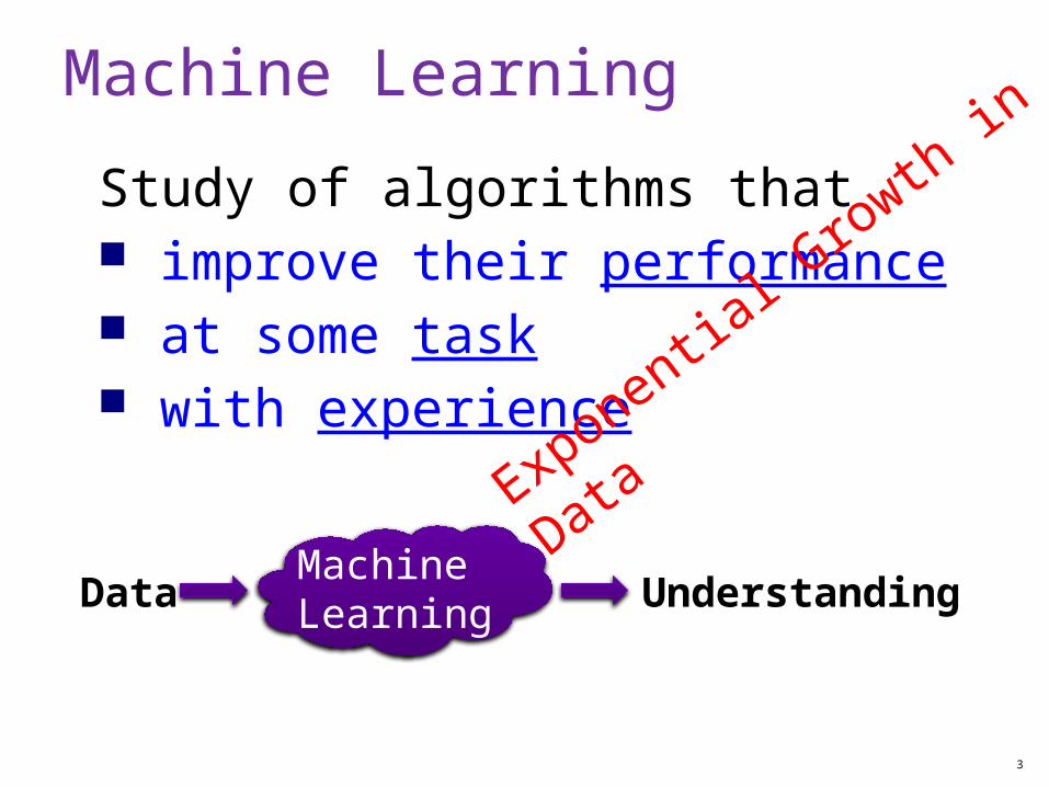
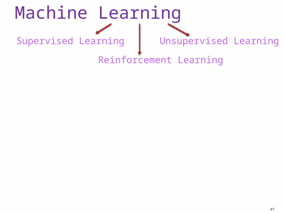
Machine Learning

Study of algorithms that improve their performance at some task with experience

Data UnderstandingMachine Learning

Exponentia

l Growth in

Data

4

Supremacy of Machine Learning Machine learning is preferred approach to

Speech recognition, Natural language processing Web search – result ranking Computer vision Medical outcomes analysis Robot control Computational biology Sensor networks …

This trend is accelerating Improved machine learning algorithms Improved data capture, networking, faster computers Software too complex to write by hand New sensors / IO devices Demand for self-customization to user, environment

5

Reinforcement Learning

©2005-2009 Carlos Guestrin

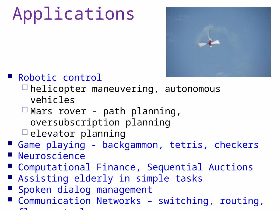
Applications

Robotic control helicopter maneuvering, autonomous vehicles Mars rover - path planning, oversubscription planning elevator planning

Game playing - backgammon, tetris, checkers Neuroscience Computational Finance, Sequential Auctions Assisting elderly in simple tasks Spoken dialog management Communication Networks – switching, routing, flow control War planning, evacuation planning

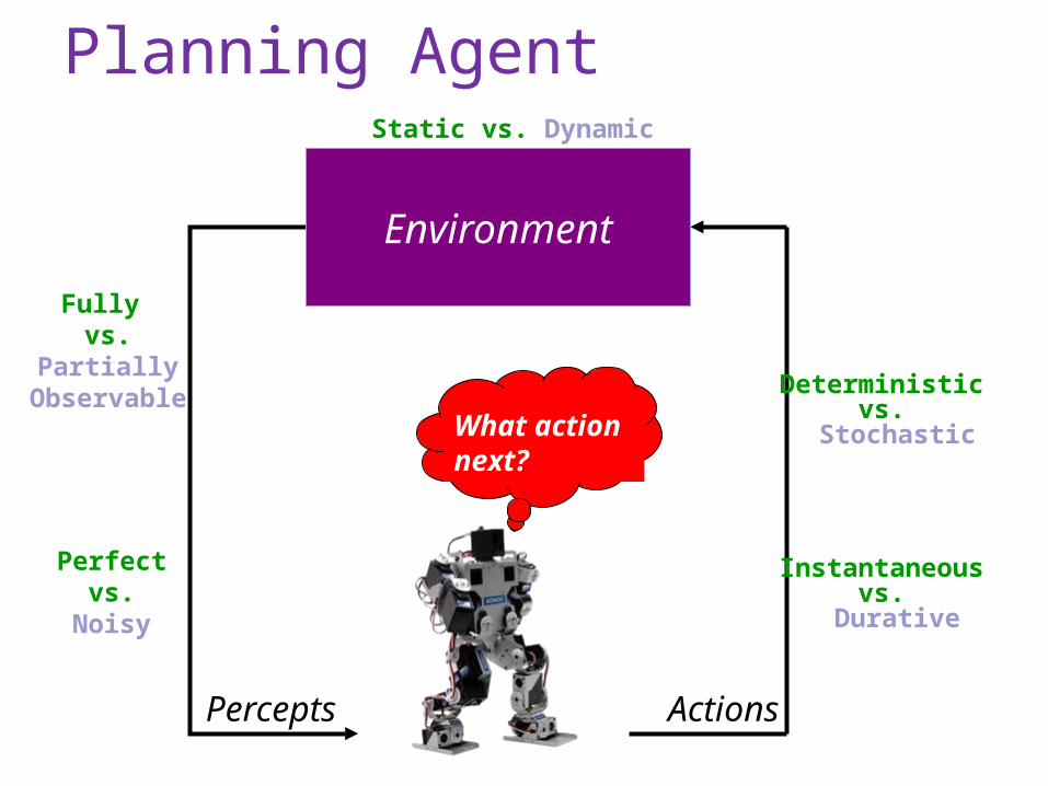
Planning Agent

What action next?

Percepts Actions

Environment

Static vs. Dynamic

Fully vs.

Partially Observable

Perfectvs.

Noisy

Deterministic vs.

Stochastic

Instantaneous vs.

Durative

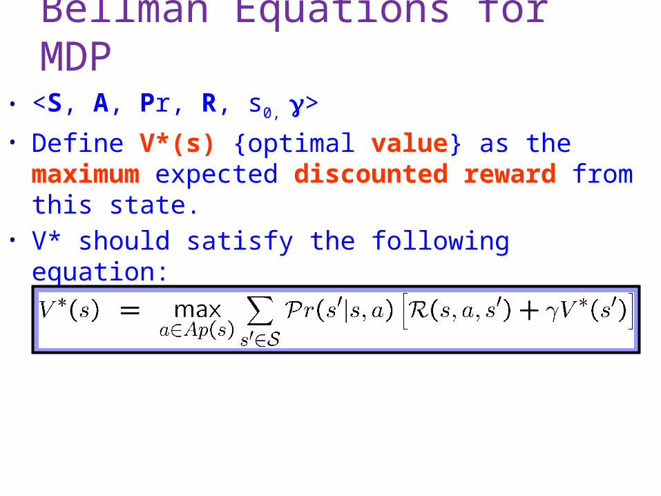
Bellman Equations for MDP

• <S, A, Pr, R, s0, >• Define V*(s) {optimal value} as the maximum

expected discounted reward from this state.• V* should satisfy the following equation:

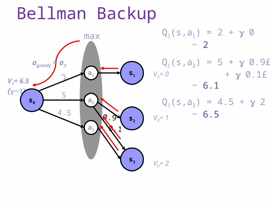
Bellman Backup

V0= 0

V0= 1

V0= 2

Q1(s,a1) = 2 + 0 ~ 2

Q1(s,a2) = 5 + 0.9£ 1 + 0.1£ 2 ~ 6.1

Q1(s,a3) = 4.5 + 2 ~ 6.5

max

V1= 6.5

(~1)

agreedy = a3

2

4.5

5a2

a1

a3

s0

s1

s2

s3

0.9

0.1

Summary RL

Bellman Equation Value iteration Credit assignment problem Explorqtion / exploitation tradeoff

Greedy in limit of infinite exploration Optomistic exploration

12

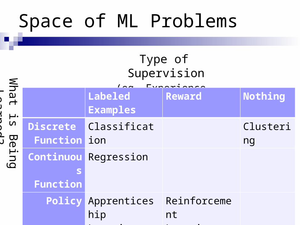
Space of ML Problems

What is B

eing Learned?

Type of Supervision (eg, Experience, Feedback)

LabeledExamples

Reward Nothing

Discrete Function

Classification Clustering

Continuous Function

Regression

Policy Apprenticeship Learning

ReinforcementLearning

13

Generalization

Hypotheses must generalize to correctly classify instances not in the training data.

Simply memorizing training examples is a consistent hypothesis that does not generalize.

Learning as function approximation

What’s a good approximation?

14

© Daniel S. Weld 15

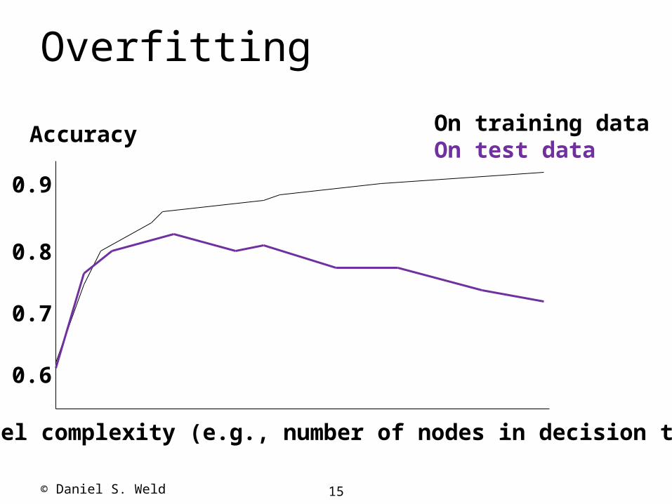
Overfitting

Accuracy

0.9

0.8

0.7

0.6

On training dataOn test data

Model complexity (e.g., number of nodes in decision tree)

16

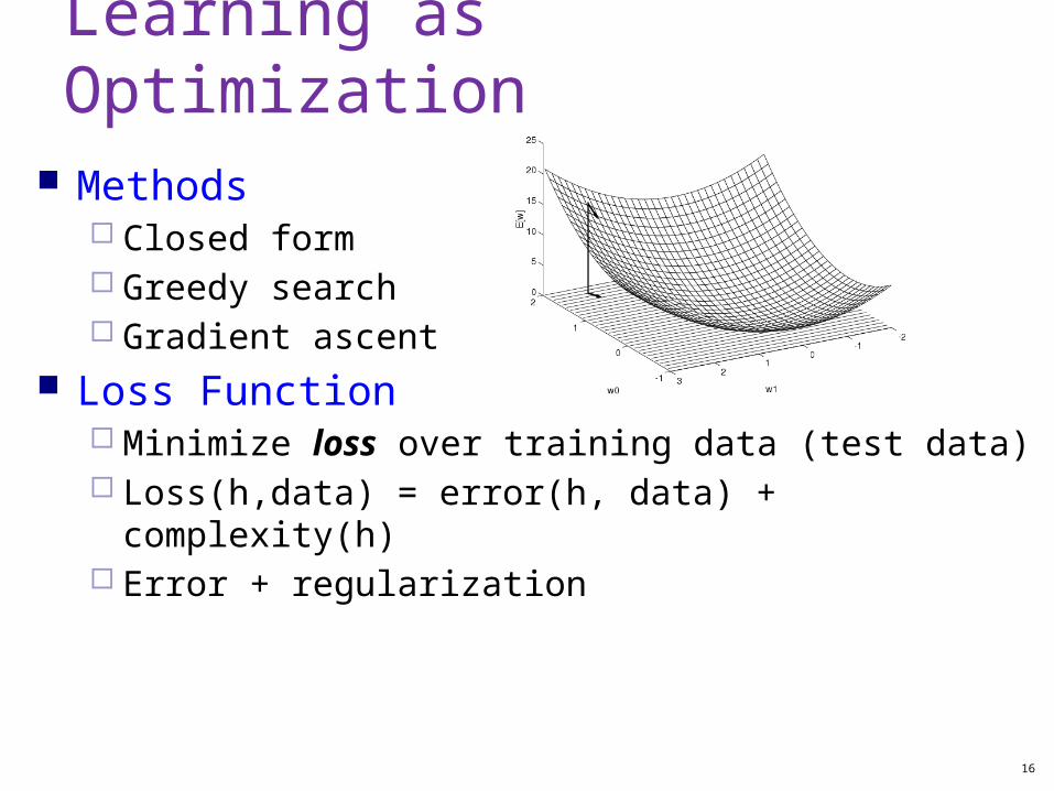
Learning as Optimization

Methods Closed form Greedy search Gradient ascent

Loss Function Minimize loss over training data (test data) Loss(h,data) = error(h, data) + complexity(h) Error + regularization

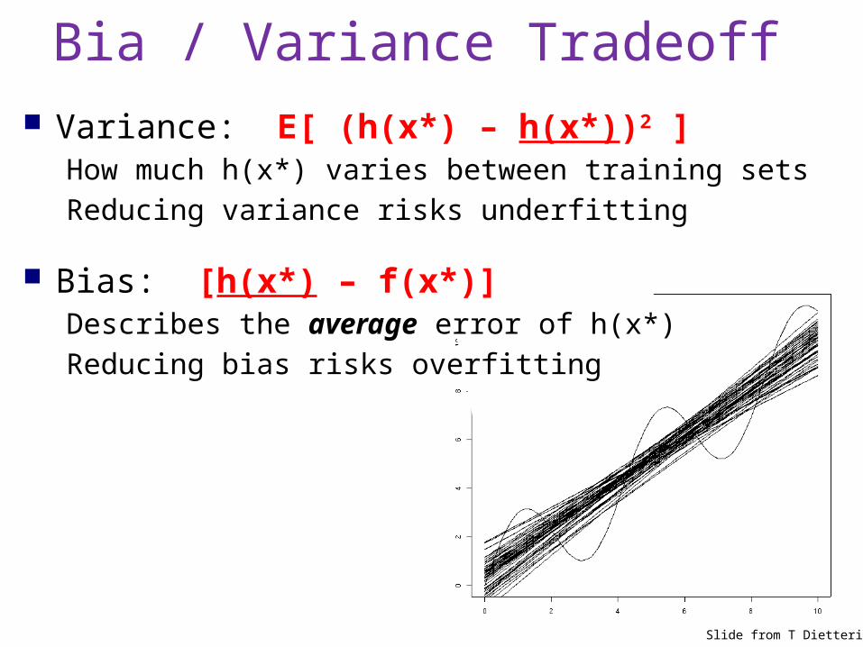
Bia / Variance Tradeoff

Slide from T Dietterich

Variance: E[ (h(x*) – h(x*))2 ]How much h(x*) varies between training sets

Reducing variance risks underfitting

Bias: [h(x*) – f(x*)]Describes the average error of h(x*)

Reducing bias risks overfitting

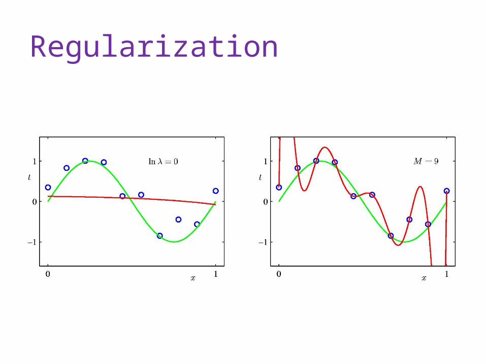
Regularization

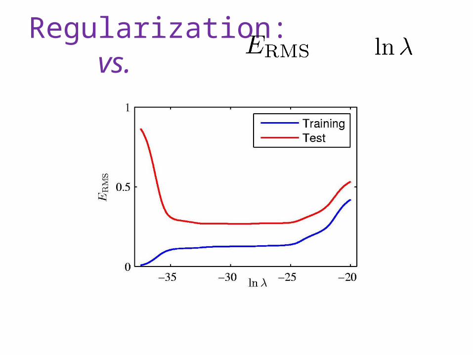
Regularization: vs.

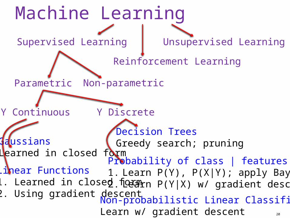
Machine Learning

20

Supervised Learning

Y Discrete Y Continuous

GaussiansLearned in closed form

Linear Functions1. Learned in closed form2. Using gradient descent

Decision TreesGreedy search; pruning

Probability of class | features1. Learn P(Y), P(X|Y); apply Bayes 2. Learn P(Y|X) w/ gradient descent

Parametric

Reinforcement Learning

Unsupervised Learning

Non-parametric

Non-probabilistic Linear ClassifierLearn w/ gradient descent

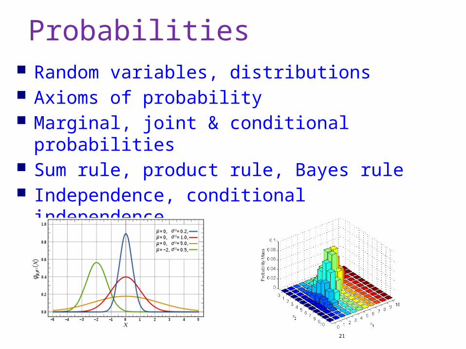
Probabilities Random variables, distributions Axioms of probability Marginal, joint & conditional probabilities Sum rule, product rule, Bayes rule Independence, conditional independence

21

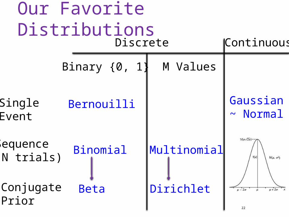
Our Favorite Distributions

22

Discrete Continuous

Binary {0, 1} M Values

SingleEvent

Sequence(N trials)

Bernouilli

Binomial Multinomial

Beta DirichletConjugatePrior

Gaussian~ Normal

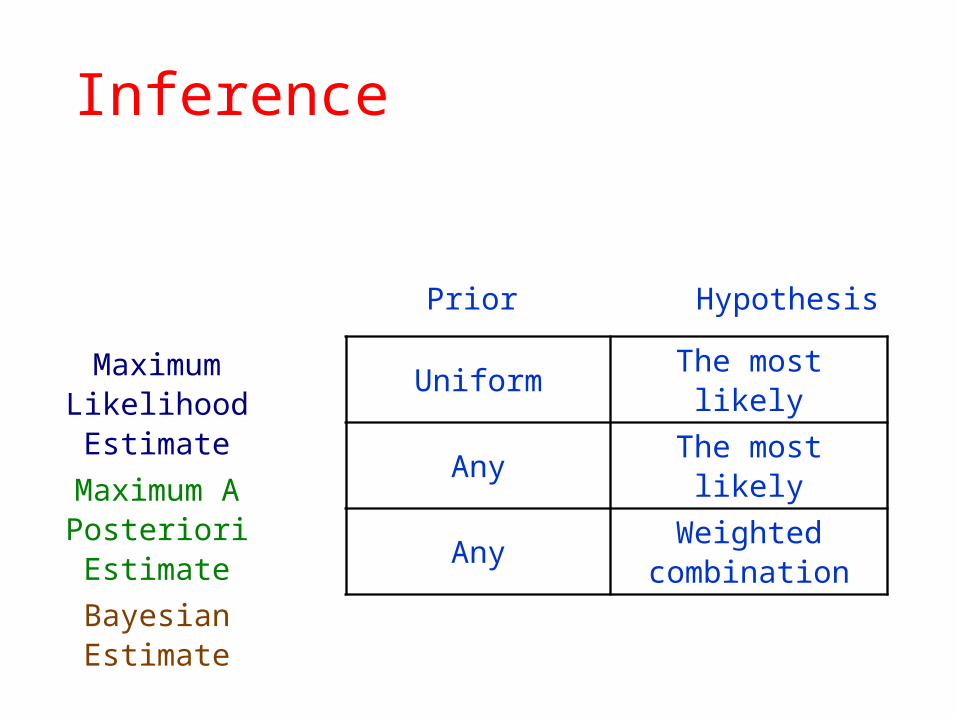
Inference

Prior Hypothesis

Maximum Likelihood Estimate

Maximum A Posteriori Estimate

Bayesian Estimate

Uniform The most likely

Any The most likely

Any Weighted combination

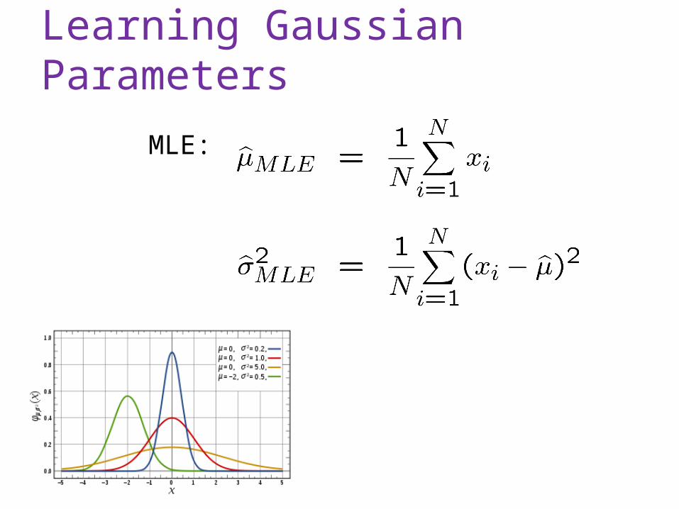
Learning Gaussian Parameters

MLE:

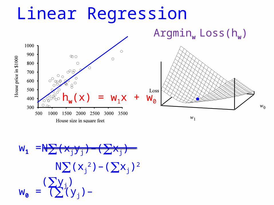
Linear Regression

hw(x) = w1x + w0

w1 =

Argminw Loss(hw)

w0 = ((yj)–w1(xj)/N

N(xjyj)–(xj)(yj)

N(xj2)–(xj)2

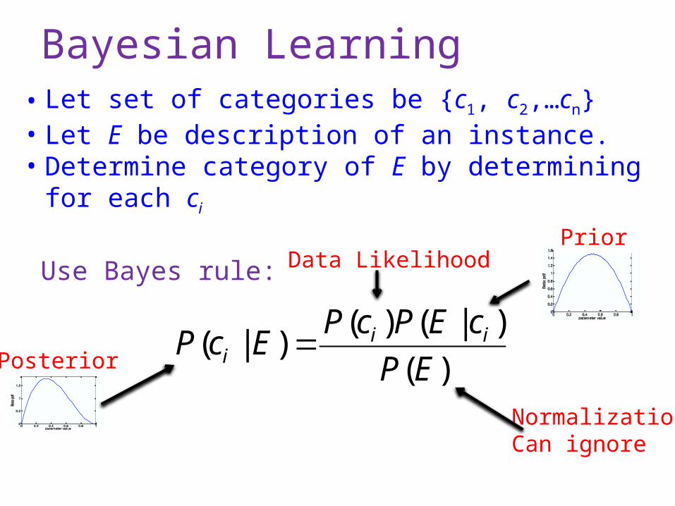
Bayesian Learning

Use Bayes rule:Prior

NormalizationCan ignore

Data Likelihood

Posterior

• Let set of categories be {c1, c2,…cn}• Let E be description of an instance.• Determine category of E by determining for each ci

)(

)|()()|(

EP

cEPcPEcP ii

i

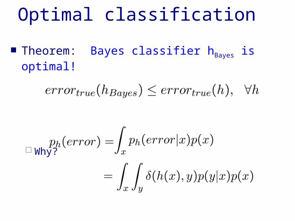
Optimal classification

Theorem: Bayes classifier hBayes is optimal!

Why?

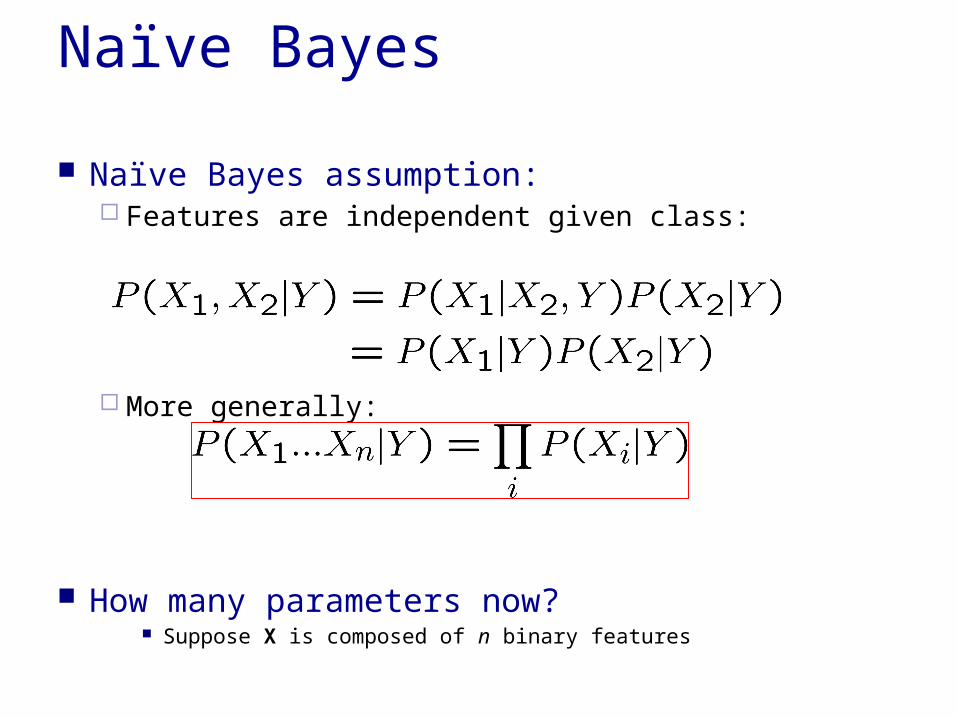
Naïve Bayes

Naïve Bayes assumption: Features are independent given class:

More generally:

How many parameters now? Suppose X is composed of n binary features

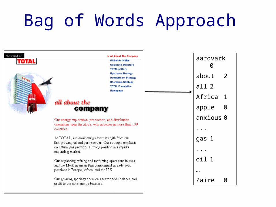
Bag of Words Approach

aardvark 0

about 2

all 2

Africa 1

apple 0

anxious 0

...

gas 1

...

oil 1

…

Zaire 0

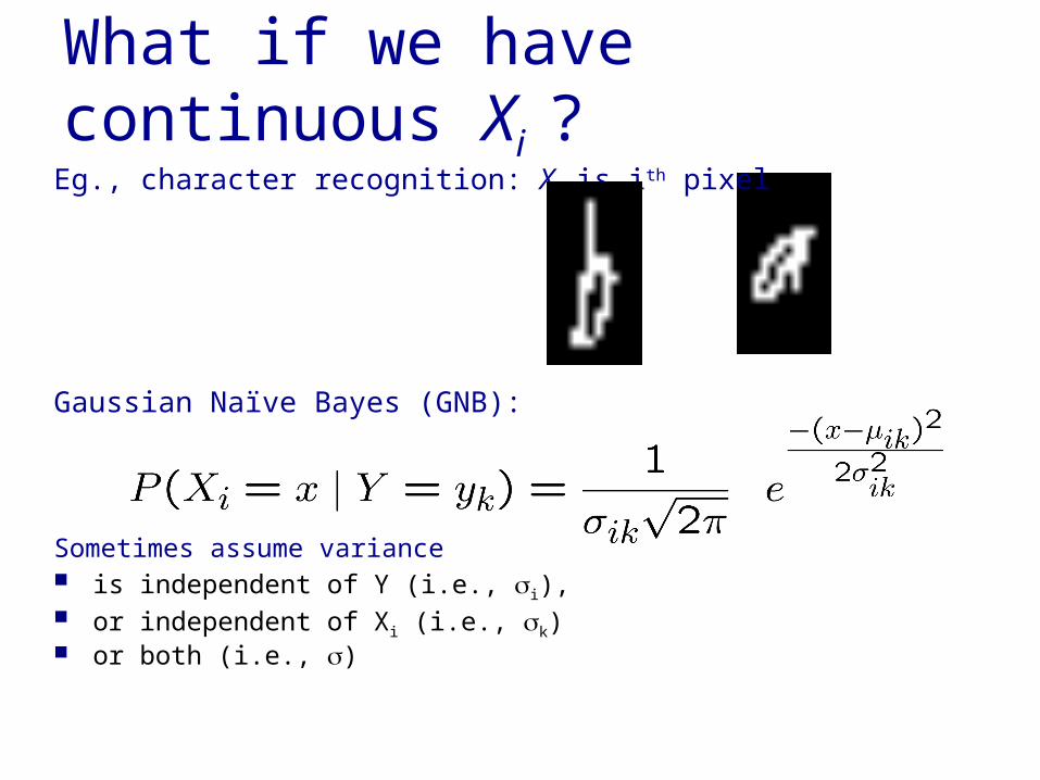
What if we have continuous Xi ?Eg., character recognition: Xi is ith pixel

Gaussian Naïve Bayes (GNB):

Sometimes assume variance is independent of Y (i.e., i), or independent of Xi (i.e., k) or both (i.e., )

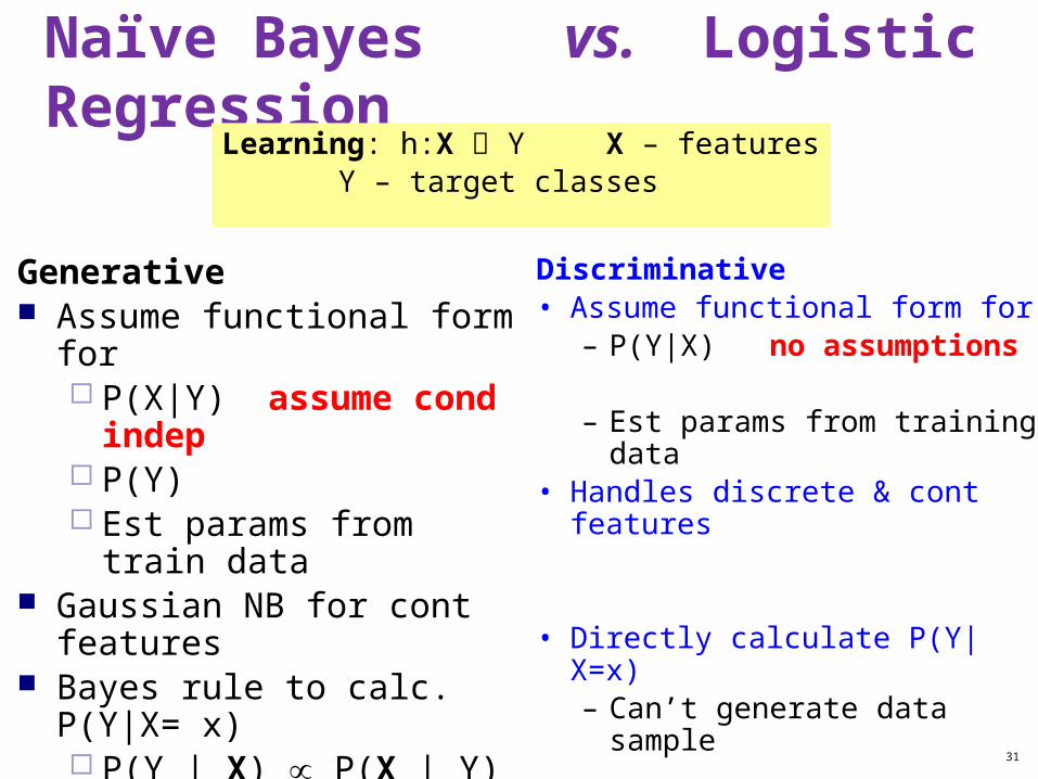
Naïve Bayes vs. Logistic Regression

Generative Assume functional form for

P(X|Y) assume cond indep P(Y) Est params from train data

Gaussian NB for cont features Bayes rule to calc. P(Y|X= x)

P(Y | X) P(X | Y) P(Y) Indirect computation

Can also generate a sample of the data

31

Discriminative• Assume functional form for

– P(Y|X) no assumptions

– Est params from training data• Handles discrete & cont features

• Directly calculate P(Y|X=x)– Can’t generate data sample

Learning: h:X Y X – features Y – target classes

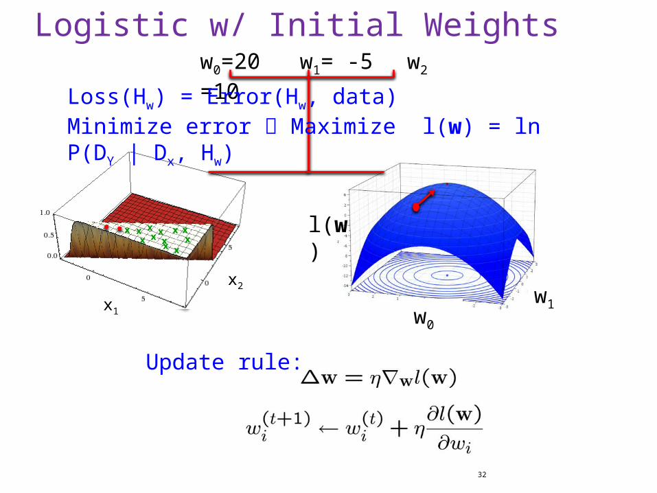
Logistic w/ Initial Weights

32

w0=20 w1= -5 w2 =10

x x x xx x x

x x

x xx

x1

x2

Update rule:

w0

w1

l(w)

Loss(Hw) = Error(Hw, data)Minimize error Maximize l(w) = ln P(DY | Dx, Hw)

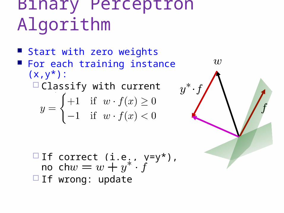
Binary Perceptron Algorithm

Start with zero weights For each training instance (x,y*):

Classify with current weights

If correct (i.e., y=y*), no change! If wrong: update

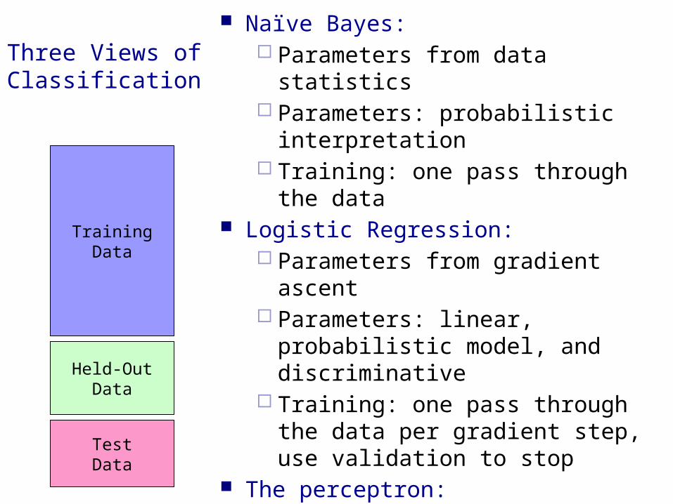
Three Views of Classification

Naïve Bayes: Parameters from data statistics Parameters: probabilistic

interpretation Training: one pass through the data

Logistic Regression: Parameters from gradient ascent Parameters: linear, probabilistic

model, and discriminative Training: one pass through the data

per gradient step, use validation to stop

The perceptron: Parameters from reactions to

mistakes Parameters: discriminative

interpretation Training: go through the data until

held-out accuracy maxes out

TrainingData

Held-OutData

TestData

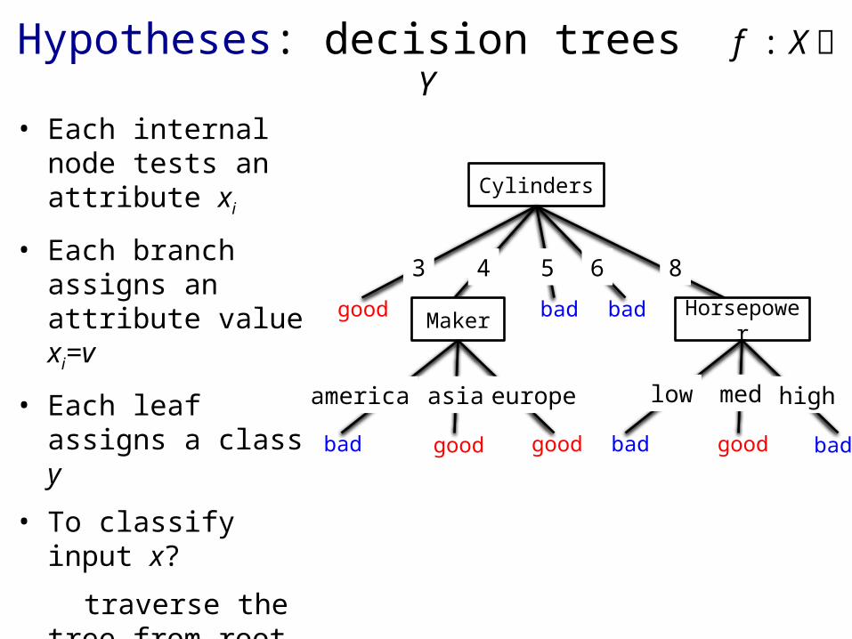
Hypotheses: decision trees f : X Y

• Each internal node tests an attribute xi

• Each branch assigns an attribute value xi=v

• Each leaf assigns a class y

• To classify input x?

traverse the tree from root to leaf, output the labeled y

Cylinders

3 4 5 6 8

good bad badMaker Horsepower

low med highamerica asia europe

bad badgoodgood goodbad

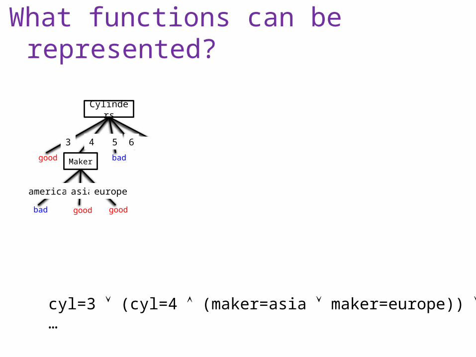
What functions can be represented?

cyl=3 (cyl=4 (maker=asia maker=europe)) …

Cylinders

3 4 5 6 8

good bad badMakerHorsepow

er

low med highamerica asia europe

bad badgoodgood goodbad

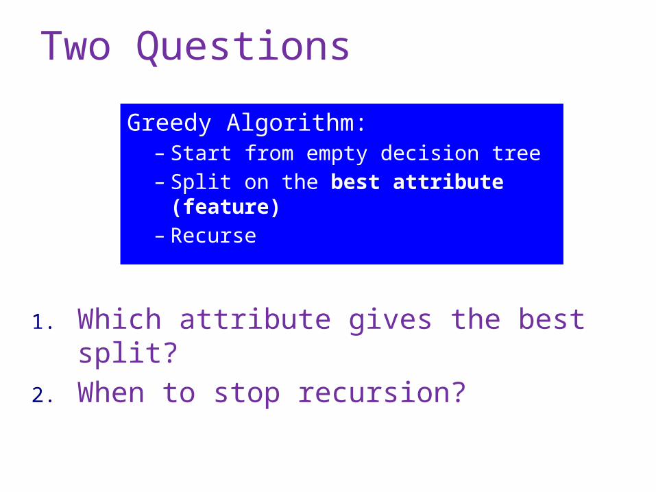
Two Questions

1. Which attribute gives the best split?

2. When to stop recursion?

Greedy Algorithm:– Start from empty decision tree– Split on the best attribute (feature)– Recurse

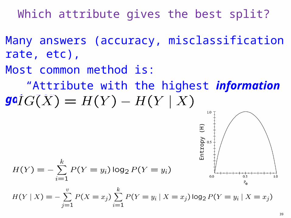
Which attribute gives the best split?

Many answers (accuracy, misclassification rate, etc),

Most common method is:

“Attribute with the highest information gain, IG”

39

Ent

rop

y (H

)

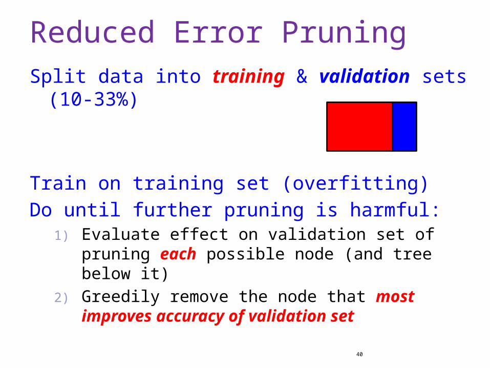
Reduced Error PruningSplit data into training & validation sets (10-33%)

Train on training set (overfitting)

Do until further pruning is harmful:1) Evaluate effect on validation set of pruning each

possible node (and tree below it)

2) Greedily remove the node that most improves accuracy of validation set

40

© Daniel S. Weld41

Ensembles of Classifiers

Traditional approach: Use one classifier

Can one do better?Approaches:

• Cross-validated committees• Bagging• Boosting• Stacking

© Daniel S. Weld42

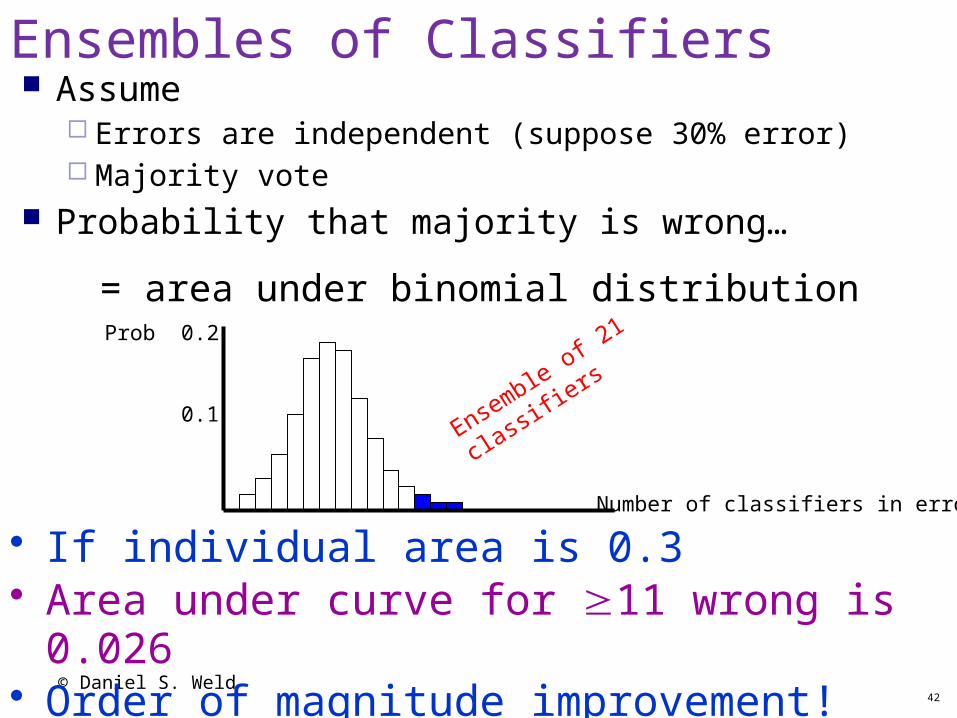
Ensembles of Classifiers Assume

Errors are independent (suppose 30% error) Majority vote

Probability that majority is wrong…

• If individual area is 0.3• Area under curve for 11 wrong is 0.026• Order of magnitude improvement!

Ensemble of 21

classifiers

Prob 0.2

0.1

Number of classifiers in error

= area under binomial distribution

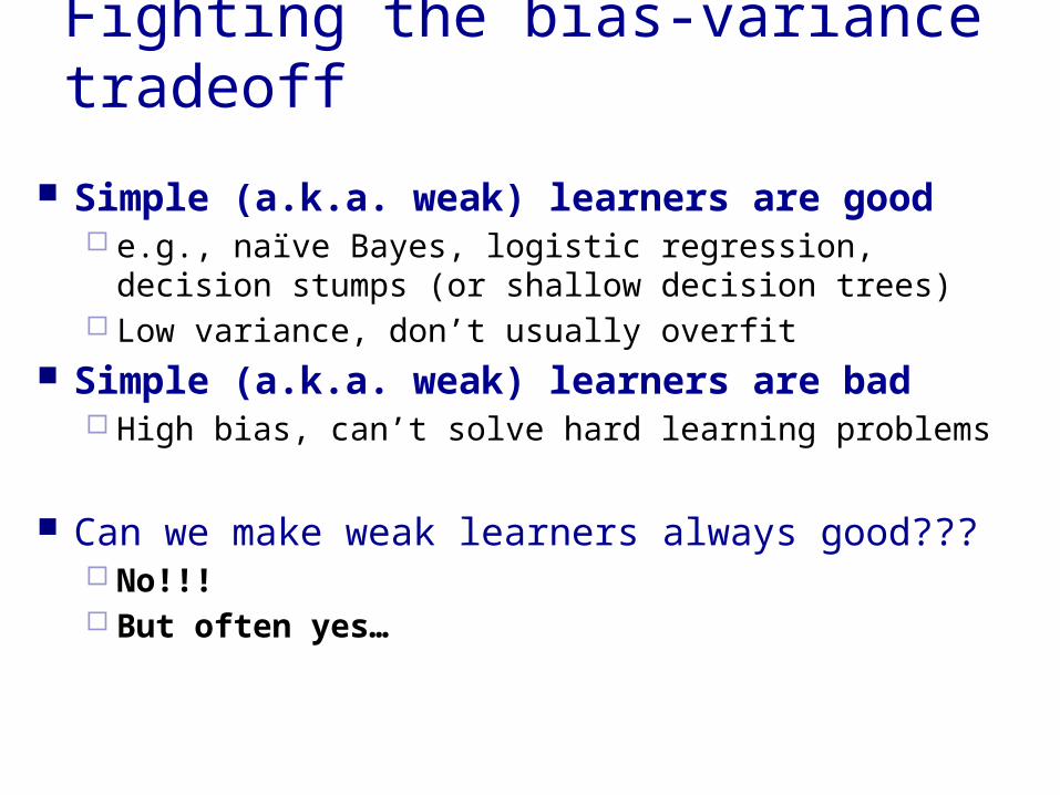
Fighting the bias-variance tradeoff

Simple (a.k.a. weak) learners are good e.g., naïve Bayes, logistic regression, decision stumps

(or shallow decision trees) Low variance, don’t usually overfit

Simple (a.k.a. weak) learners are bad High bias, can’t solve hard learning problems

Can we make weak learners always good??? No!!! But often yes…

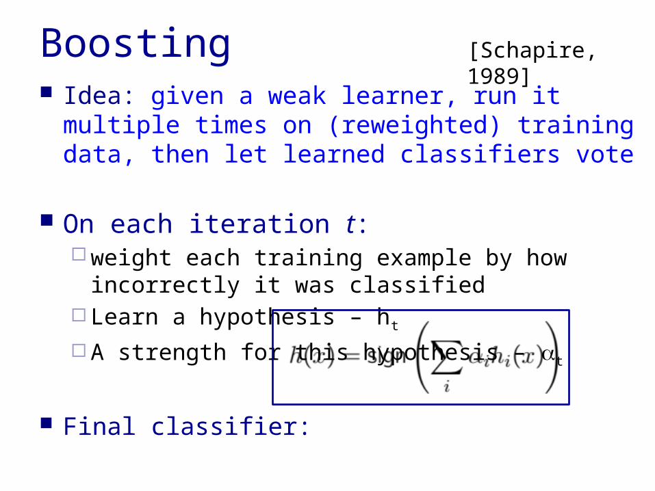
Boosting Idea: given a weak learner, run it multiple times on

(reweighted) training data, then let learned classifiers vote

On each iteration t: weight each training example by how incorrectly it

was classified Learn a hypothesis – ht

A strength for this hypothesis – t

Final classifier:

[Schapire, 1989]

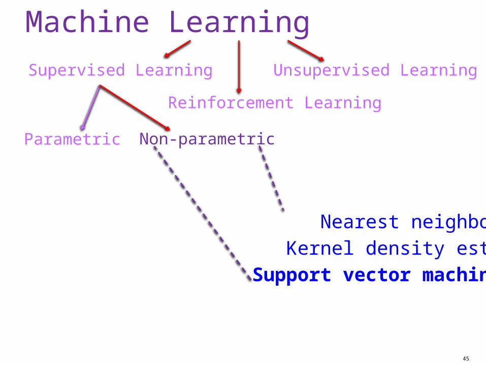
Machine Learning

45

Supervised Learning

Parametric

Reinforcement Learning

Unsupervised Learning

Non-parametric

Nearest neighbor

Kernel density estimation

Support vector machines

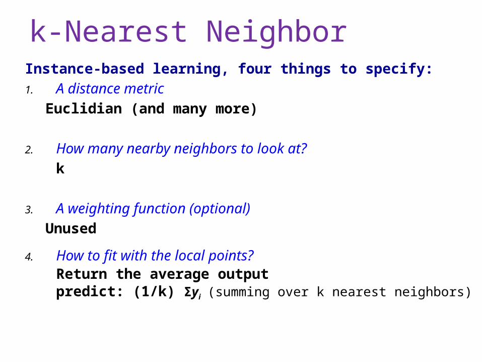
k-Nearest NeighborInstance-based learning, four things to specify:1. A distance metric

Euclidian (and many more)

2. How many nearby neighbors to look at?

k

3. A weighting function (optional)

Unused

4. How to fit with the local points?Return the average output predict: (1/k) Σyi (summing over k nearest neighbors)

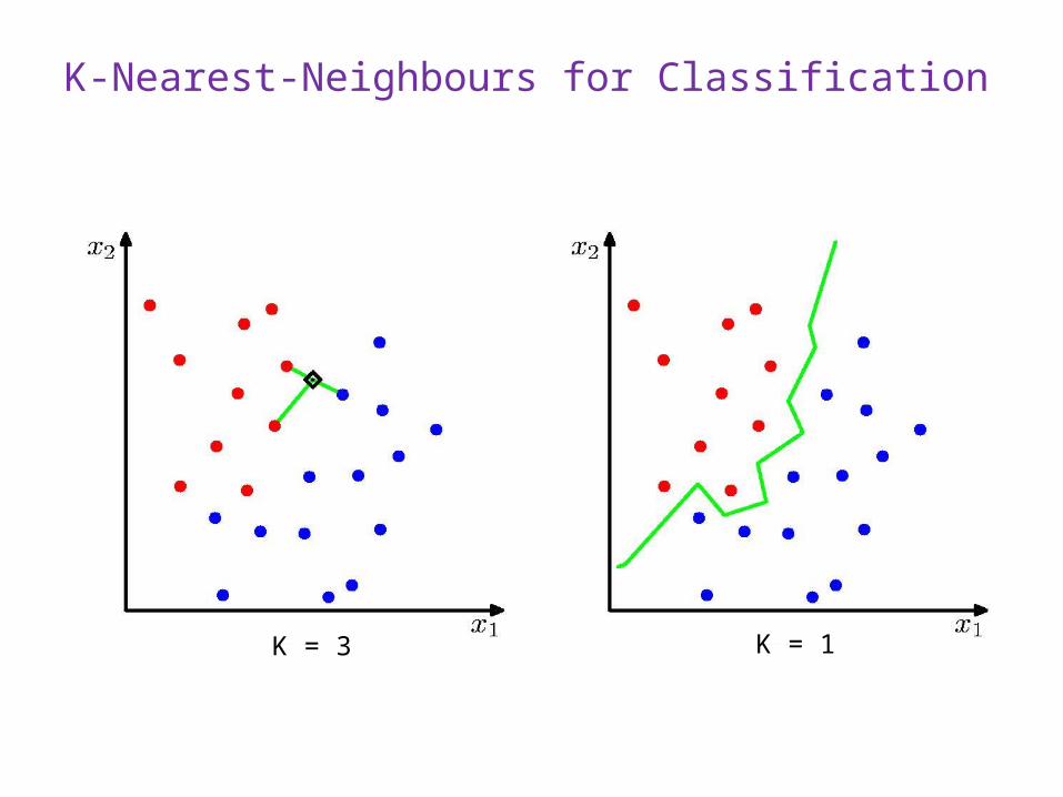
K-Nearest-Neighbours for Classification

K = 1K = 3

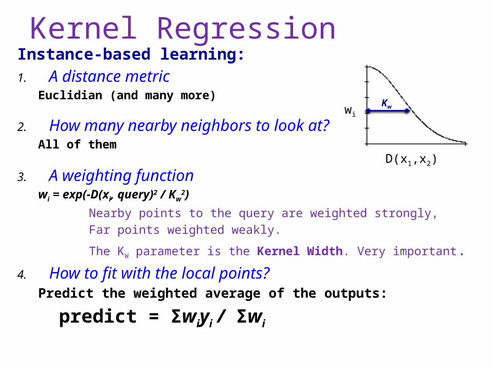
Kernel RegressionInstance-based learning:1. A distance metric

Euclidian (and many more)

2. How many nearby neighbors to look at?All of them

3. A weighting functionwi = exp(-D(xi, query)2 / Kw

2)

Nearby points to the query are weighted strongly,

Far points weighted weakly.

The KW parameter is the Kernel Width. Very important.

4. How to fit with the local points?Predict the weighted average of the outputs:

predict = Σwiyi / Σwi

D(x1,x2)

wi

Kw

49

Support Vector Machines

Key insight Max Margin

Clever trick Kernel trick

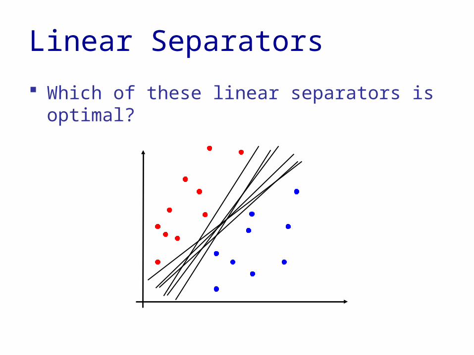
Linear Separators

Which of these linear separators is optimal?

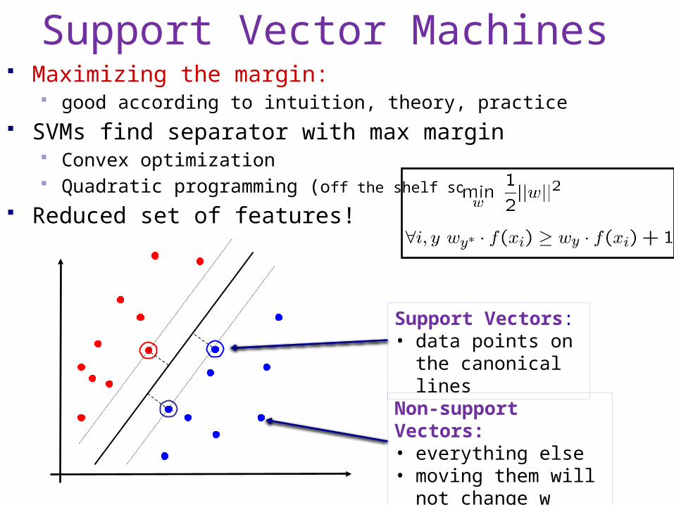
Support Vector Machines Maximizing the margin:

good according to intuition, theory, practice SVMs find separator with max margin

Convex optimization Quadratic programming (off the shelf solns)

Reduced set of features!

Support Vectors:• data points on the

canonical lines

Non-support Vectors:• everything else• moving them will not

change w

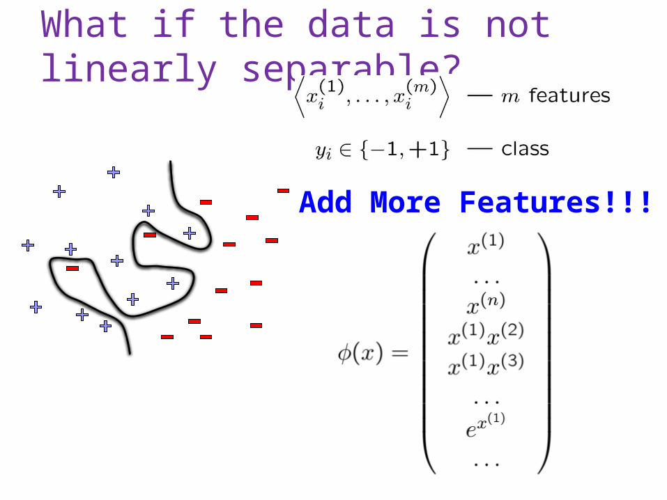
What if the data is not linearly separable?

Add More Features!!!

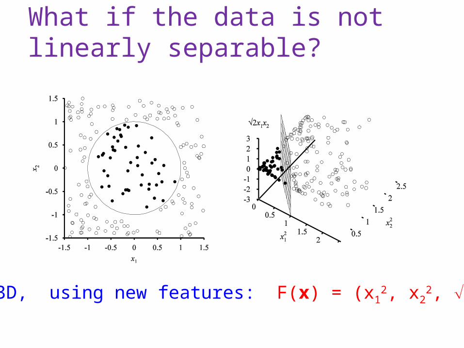
What if the data is not linearly separable?

2D 3D, using new features: F(x) = (x12, x2

2, 2 x1x2)

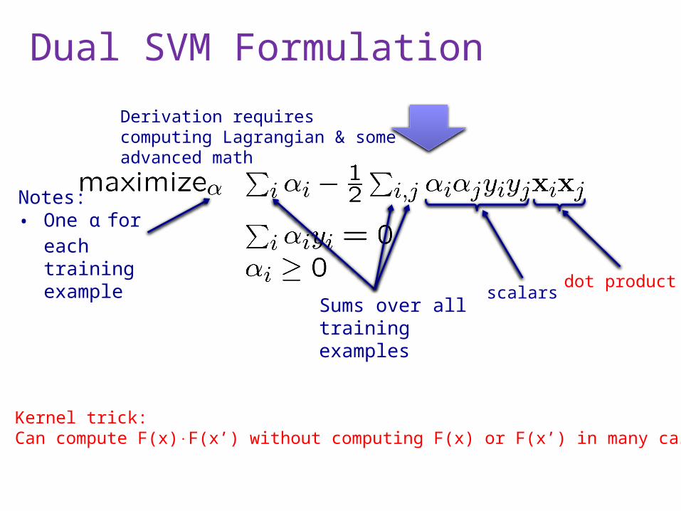
Dual SVM Formulation

Derivation requires computing Lagrangian & some advanced math

Notes: • One α for

each training example

Sums over all training examples

dot productscalars

Kernel trick:Can compute F(x)F(x’) without computing F(x) or F(x’) in many cases

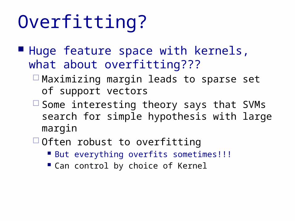
Overfitting? Huge feature space with kernels, what about

overfitting??? Maximizing margin leads to sparse set of support

vectors Some interesting theory says that SVMs search for

simple hypothesis with large margin Often robust to overfitting

But everything overfits sometimes!!! Can control by choice of Kernel

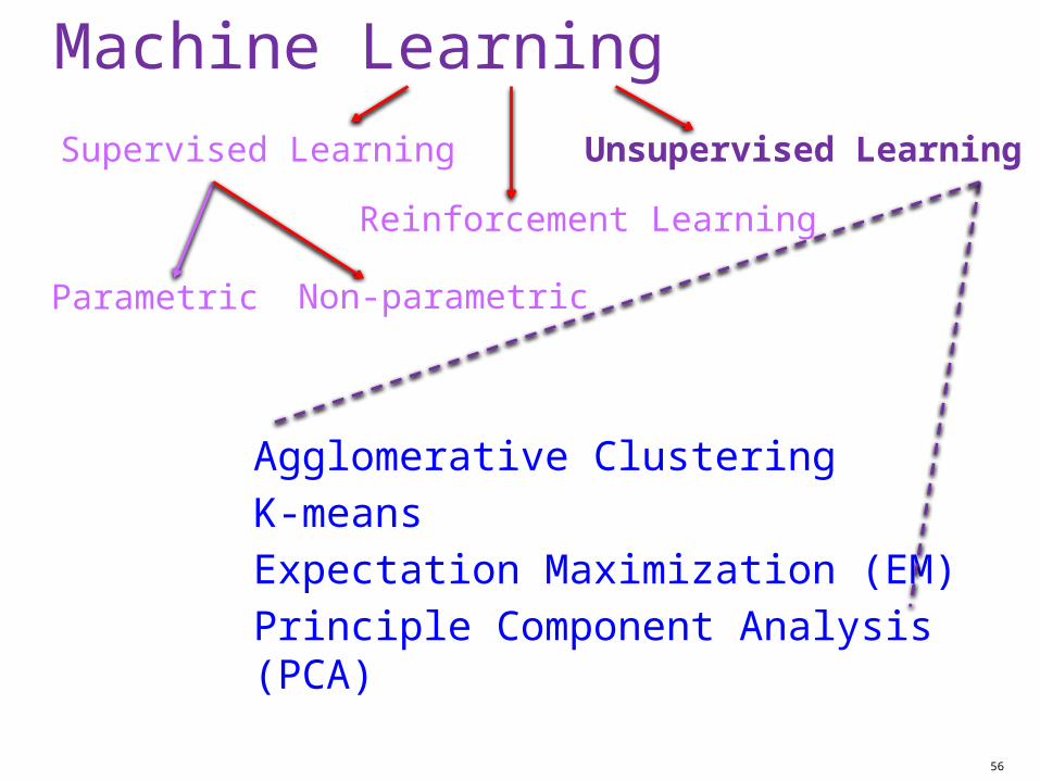
Machine Learning

56

Supervised Learning

Parametric

Reinforcement Learning

Unsupervised Learning

Non-parametric

Agglomerative Clustering

K-means

Expectation Maximization (EM)

Principle Component Analysis (PCA)

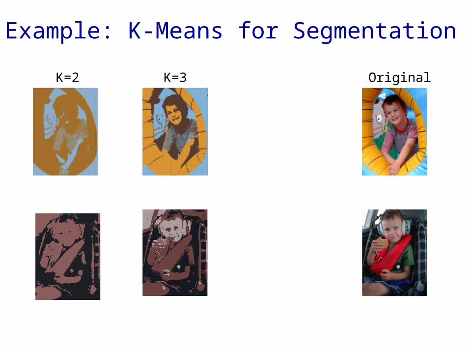
Example: K-Means for Segmentation

K=2 K=3 K=10 Original

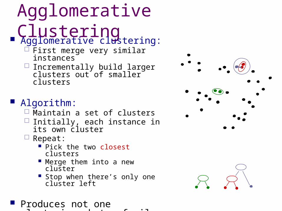
Agglomerative Clustering Agglomerative clustering:

First merge very similar instances Incrementally build larger clusters out

of smaller clusters

Algorithm: Maintain a set of clusters Initially, each instance in its own

cluster Repeat:

Pick the two closest clusters Merge them into a new cluster Stop when there’s only one cluster left

Produces not one clustering, but a family of clusterings represented by a dendrogram

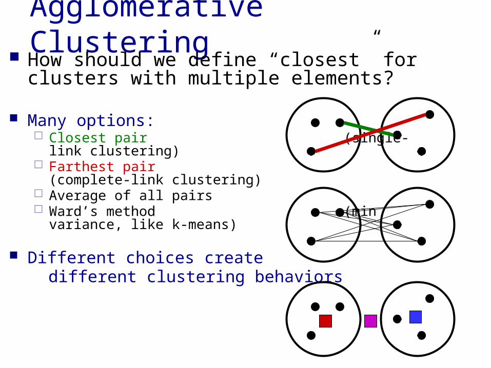
Agglomerative Clustering How should we define “closest” for clusters

with multiple elements?

Many options: Closest pair

(single-link clustering) Farthest pair

(complete-link clustering) Average of all pairs Ward’s method

(min variance, like k-means)

Different choices create different clustering behaviors

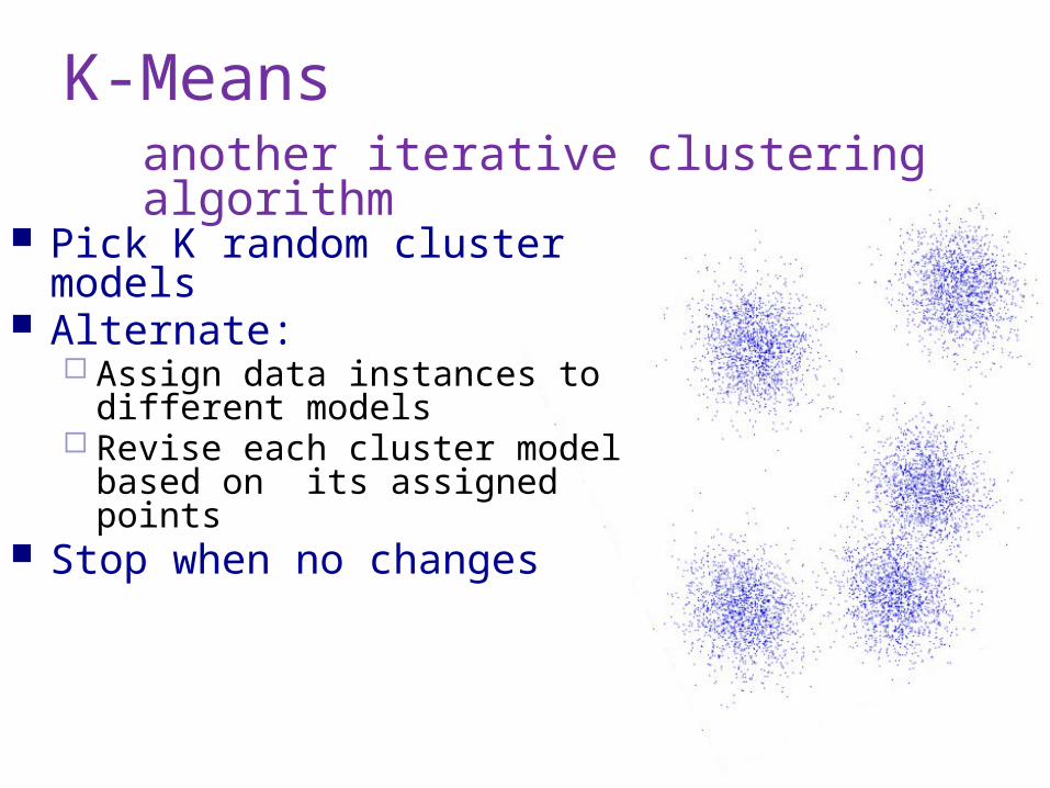
K-Means

Pick K random cluster models Alternate:

Assign data instances to different models

Revise each cluster model based on its assigned points

Stop when no changes

another iterative clustering algorithm

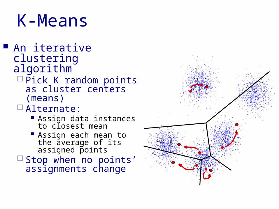
K-Means An iterative clustering

algorithm Pick K random points as

cluster centers (means) Alternate:

Assign data instances to closest mean

Assign each mean to the average of its assigned points

Stop when no points’ assignments change

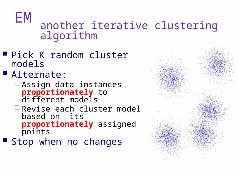
EM

Pick K random cluster models Alternate:

Assign data instances proportionately to different models

Revise each cluster model based on its proportionately assigned points

Stop when no changes

another iterative clustering algorithm

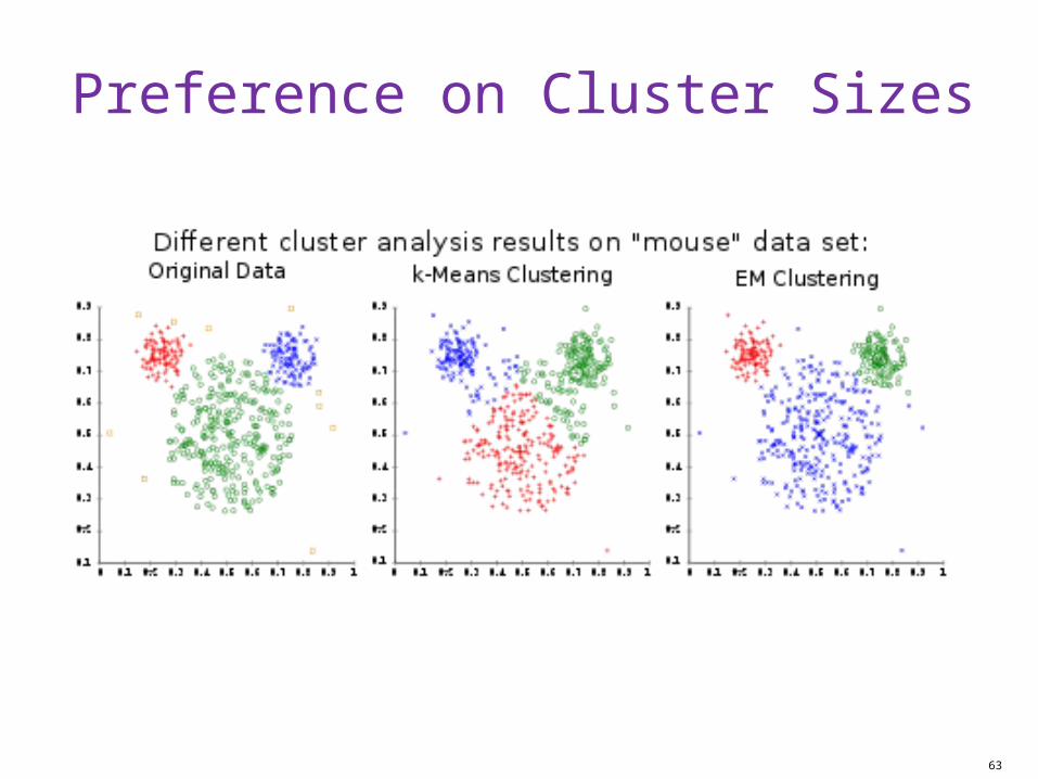
Preference on Cluster Sizes

63

Feature Selection

Want to learn f:XY X=<X1,…,Xn> but some features are more important than others

Approach: select subset of features to be used by learning algorithm Score each feature (or sets of features) Select set of features with best score

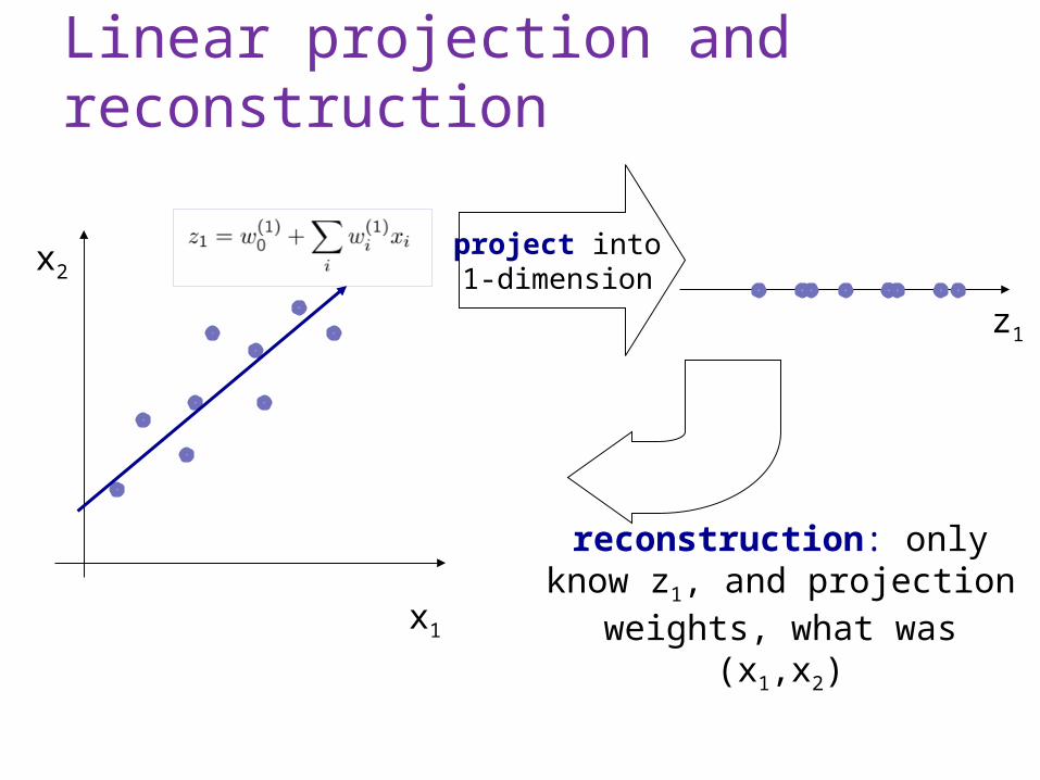
Linear projection and reconstruction

x1

x2project into1-dimension

z1

reconstruction: only know z1, and projection weights, what

was (x1,x2)

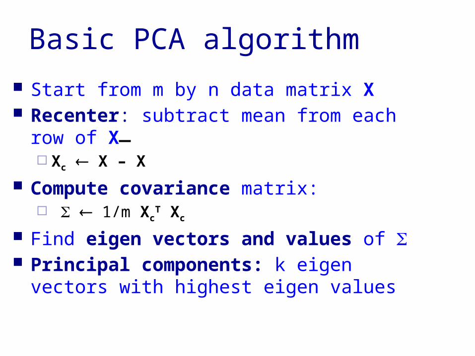
Basic PCA algorithm

Start from m by n data matrix X Recenter: subtract mean from each row of X

Xc X – X

Compute covariance matrix: 1/m Xc

T Xc

Find eigen vectors and values of Principal components: k eigen vectors with

highest eigen values

Machine Learning

67

Supervised Learning

Reinforcement Learning

Unsupervised Learning

© Daniel S. Weld68

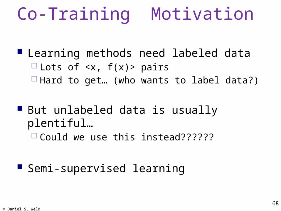
Co-Training Motivation

Learning methods need labeled data Lots of <x, f(x)> pairs Hard to get… (who wants to label data?)

But unlabeled data is usually plentiful… Could we use this instead??????

Semi-supervised learning

© Daniel S. Weld69

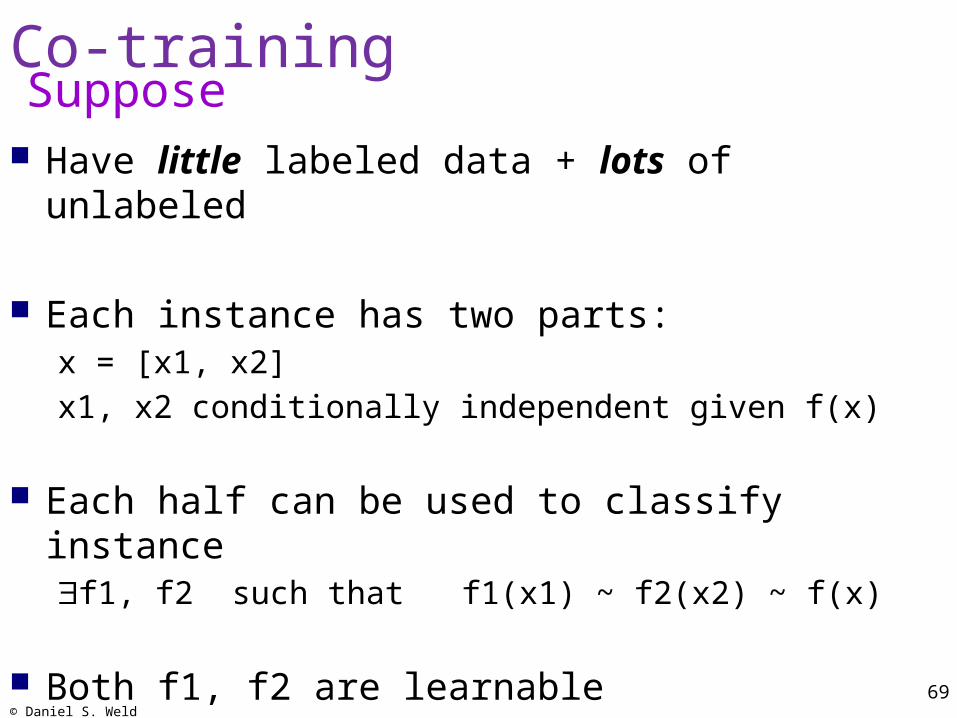
Co-training

Have little labeled data + lots of unlabeled

Each instance has two parts:x = [x1, x2]

x1, x2 conditionally independent given f(x)

Each half can be used to classify instancef1, f2 such that f1(x1) ~ f2(x2) ~ f(x)

Both f1, f2 are learnablef1 H1, f2 H2, learning algorithms A1, A2

Suppose

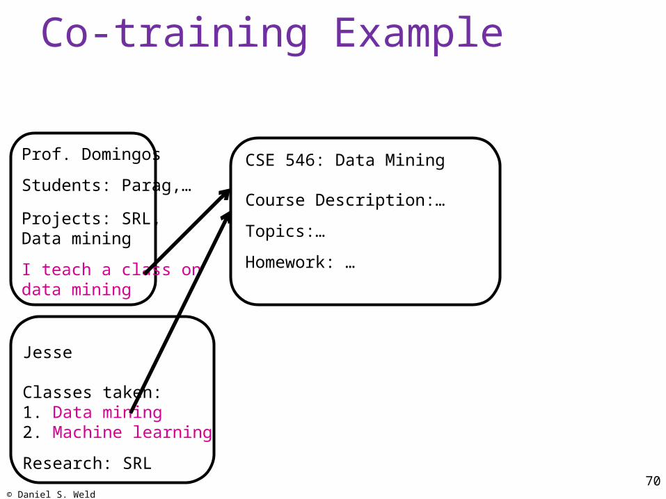
Co-training Example

© Daniel S. Weld70

Prof. Domingos

Students: Parag,…

Projects: SRL, Data mining

I teach a class on data mining

CSE 546: Data Mining

Course Description:…

Topics:…

Homework: …

Jesse

Classes taken: 1. Data mining2. Machine learning

Research: SRL

© Daniel S. Weld71

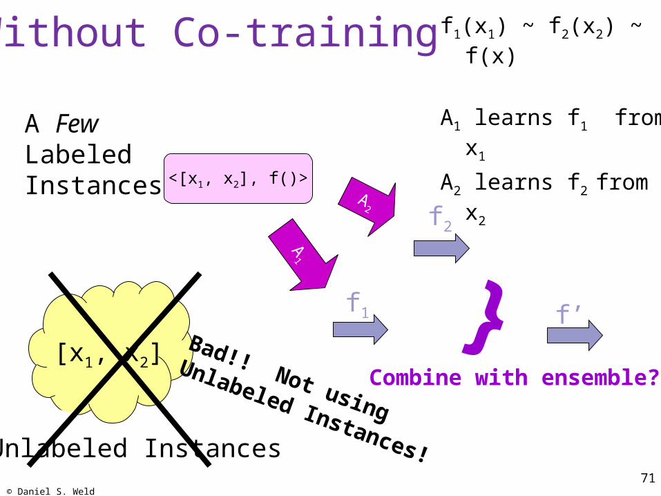
Without Co-training f1(x1) ~ f2(x2) ~ f(x)

A1 learns f1 from x1

A2 learns f2 from x2A Few Labeled Instances

[x1, x2]

f2

A2

<[x1, x2], f()>

Unlabeled Instances

A1

f1 }Combine with ensemble?

Bad!! Not using

Unlabeled Instances!

f’

© Daniel S. Weld72

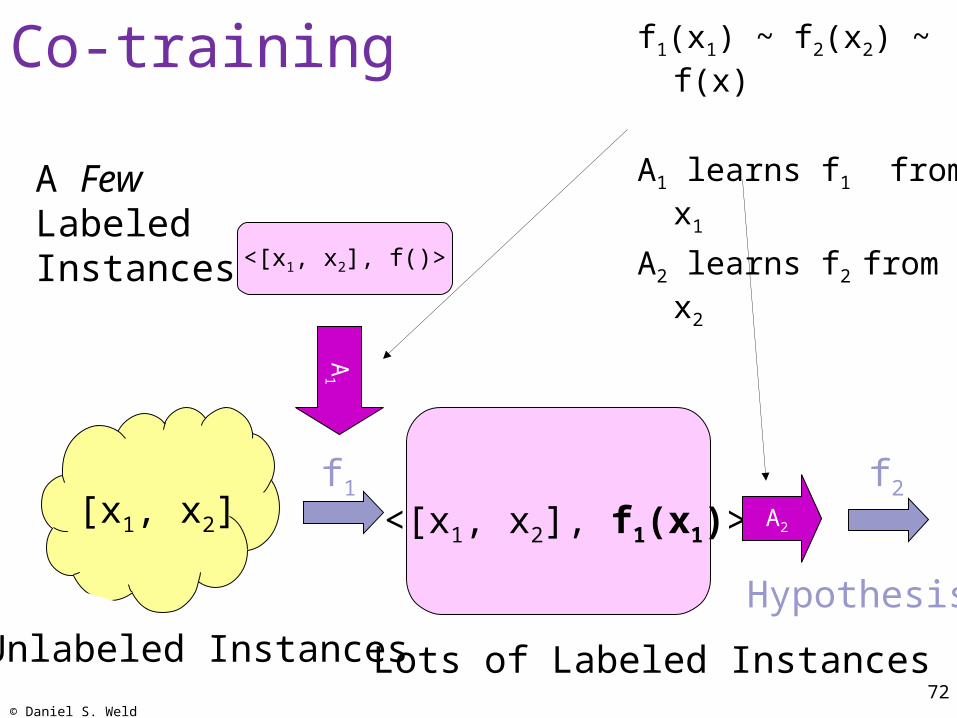
Co-training f1(x1) ~ f2(x2) ~ f(x)

A1 learns f1 from x1

A2 learns f2 from x2A Few Labeled Instances

[x1, x2]

Lots of Labeled Instances

<[x1, x2], f1(x1)>f2

Hypothesis

A2

<[x1, x2], f()>

Unlabeled InstancesA

1

f1

© Daniel S. Weld73

Observations

Can apply A1 to generate as much training data as one wants If x1 is conditionally independent of x2 / f(x),

then the error in the labels produced by A1

will look like random noise to A2 !!!

Thus no limit to quality of the hypothesis A2 can make

© Daniel S. Weld74

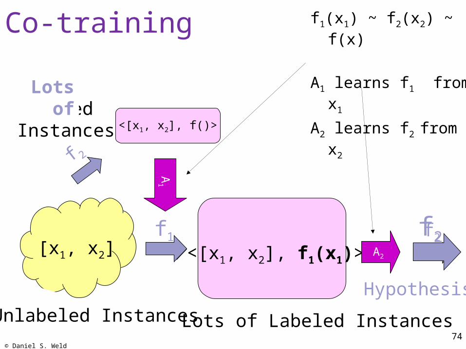
Co-training f1(x1) ~ f2(x2) ~ f(x)

A1 learns f1 from x1

A2 learns f2 from x2A Few Labeled Instances

[x1, x2]

Lots of Labeled Instances

<[x1, x2], f1(x1)>

Hypothesis

A2

<[x1, x2], f()>

Unlabeled InstancesA

1

f1 f2

f 2

Lots of

f2f1

© Daniel S. Weld75

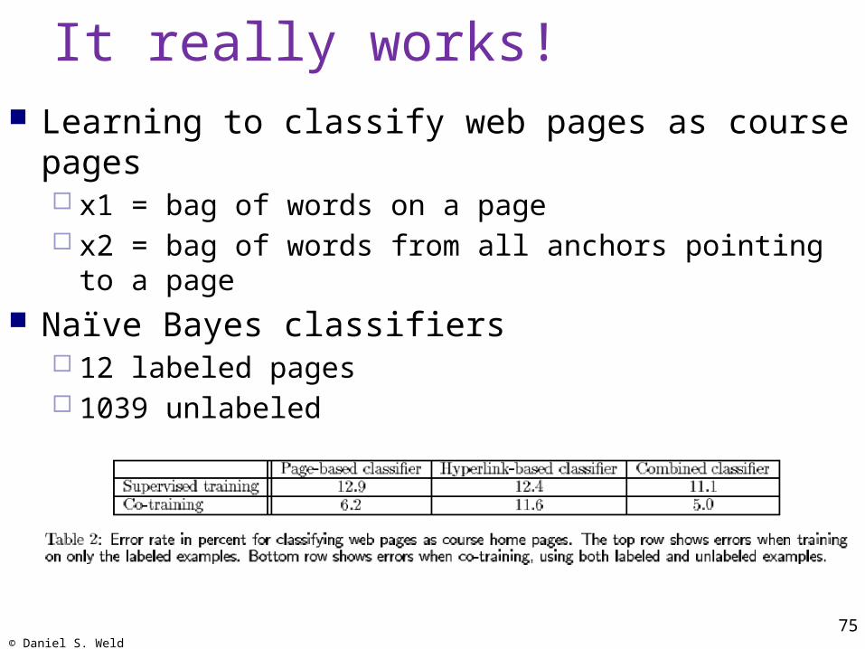
It really works! Learning to classify web pages as course pages

x1 = bag of words on a page x2 = bag of words from all anchors pointing to a page

Naïve Bayes classifiers 12 labeled pages 1039 unlabeled