Embed Size (px)
Citation preview

Improved Matrix Uncertainty Selector
Mathieu Rosenbaum1 and Alexandre B. Tsybakov2,∗
1Universite Pierre et Marie Curie, Paris-6, LPMA, case courrier 188, 4 place Jussieu,75252 Paris Cedex 05, France and CREST
2CREST (ENSAE), 3, av. Pierre Larousse, 92240 Malakoff, France
Abstract: We consider the regression model with observation error in thedesign:
y = Xθ∗ + ξ,
Z = X + Ξ.
Here the random vector y ∈ Rn and the random n×pmatrix Z are observed,the n× p matrix X is unknown, Ξ is an n× p random noise matrix, ξ ∈ Rn
is a random noise vector, and θ∗ is a vector of unknown parameters to beestimated. We consider the setting where the dimension p can be muchlarger than the sample size n and θ∗ is sparse. Because of the presenceof the noise matrix Ξ, the commonly used Lasso and Dantzig selector areunstable. An alternative procedure called the Matrix Uncertainty (MU)selector has been proposed in Rosenbaum and Tsybakov (2010) in order toaccount for the noise. The properties of the MU selector have been studiedin Rosenbaum and Tsybakov (2010) for sparse θ∗ under the assumptionthat the noise matrix Ξ is deterministic and its values are small. In thispaper, we propose a modification of the MU selector when Ξ is a randommatrix with zero-mean entries having the variances that can be estimated.This is, for example, the case in the model where the entries ofX are missingat random. We show both theoretically and numerically that, under theseconditions, the new estimator called the Compensated MU selector achievesbetter accuracy of estimation than the original MU selector.
AMS 2000 subject classifications: Primary 62J05; secondary 62F12.Keywords and phrases: Sparsity, MU selector, matrix uncertainty, errors-in-variables model, measurement error, restricted eigenvalue assumption,missing data.
1. Introduction
We consider the model
y = Xθ∗ + ξ, (1)
Z = X + Ξ, (2)
where the random vector y ∈ Rn and the random n× p matrix Z are observed,the n×pmatrixX is unknown, Ξ is an n×p random noise matrix, ξ ∈ Rn is a ran-dom noise vector, θ∗ = (θ∗1 , . . . , θ
∗p) ∈ Θ is a vector of unknown parameters to be
estimated, and Θ is a given subset of Rp. We consider the problem of estimatingan s-sparse vector θ∗ (i.e., a vector θ∗ having only s non zero components), with
∗Supported in part by ANR “Parcimonie” and by PASCAL-2 Network of Excellence.
1
May 20, 2018
arX
iv:1
112.
4413
v1 [
mat
h.ST
] 1
9 D
ec 2
011
M.Rosenbaum and A.B.Tsybakov/Matrix Uncertainty Selector 2
p possibly much larger than n. If the matrix X in (1)–(2) is observed withouterror (Ξ = 0), this problem has been recently studied in numerous papers. Theproposed estimators mainly rely on `1 minimization techniques. In particular,this is the case for the widely used Lasso and Dantzig selector, see among othersCandes and Tao (2007), Bunea et al. (2007a,b), Bickel et al. (2009), Koltchin-skii (2009), the book by Buhlmann and van de Geer (2011), the lecture notes byKoltchinskii (2011), Belloni and Chernozhukov (2011) and the references citedtherein.
However, it is shown in Rosenbaum and Tsybakov (2010) that dealing witha noisy observation of the regression matrix X has severe consequences. Inparticular, the Lasso and Dantzig selector become very unstable in this context.An alternative procedure, called the matrix uncertainty selector (MU selectorfor short) is proposed in Rosenbaum and Tsybakov (2010) in order to account
for the presence of noise Ξ. The MU selector θMU is defined as a solution of theminimization problem
min{|θ|1 : θ ∈ Θ,∣∣∣ 1nZT (y − Zθ)
∣∣∣∞≤ µ|θ|1 + τ}, (3)
where | · |p denotes the `p-norm, 1 ≤ p ≤ ∞, Θ is a given subset of Rp char-acterizing the prior knowledge about θ∗, and the constants µ and τ depend onthe level of the noises Ξ and ξ respectively. If the noise terms ξ and Ξ are deter-ministic, it is suggested in Rosenbaum and Tsybakov (2010) to choose τ suchthat ∣∣∣ 1
nZT ξ
∣∣∣∞≤ τ,
and to take µ = δ(1 + δ) with δ such that
|Ξ|∞ ≤ δ,
where, for a matrix A, we denote by |A|∞ its componentwise `∞-norm.In this paper, we propose a modification of the MU selector for the model
where Ξ is a random matrix with independent and zero mean entries Ξij suchthat the sums of expectations
σ2j ,
1
n
n∑i=1
IE(Ξ2ij), 1 ≤ j ≤ p,
are finite and admit data-driven estimators. Our main example where such es-timators exist is the model with data missing at random (see below). The ideaunderlying the new estimator is the following. In the ideal setting where thereis no noise Ξ, the estimation strategy for θ∗ is based on the matrix X. Whenthere is noise this is impossible since X is not observed and so we have no otherchoice than using Z instead of X. However, it is not hard to see that underthe above assumptions on Ξ, the matrix ZTZ/n appearing in (3) contains abias induced by the diagonal entries of the matrix ΞTΞ/n whose expectationsσ2j do not vanish. If σ2
j can be estimated from the data, it is natural to make
May 20, 2018

M.Rosenbaum and A.B.Tsybakov/Matrix Uncertainty Selector 3
a bias correction. This leads to a new estimator θ defined as a solution of theminimization problem
min{|θ|1 : θ ∈ Θ,∣∣∣ 1nZT (y − Zθ) + Dθ
∣∣∣∞≤ µ|θ|1 + τ}, (4)
where D is the diagonal matrix with entries σ2j , which are estimators of σ2
j ,and µ ≥ 0 and τ ≥ 0 are constants that will be specified later. This estimatorθ will be called the Compensated MU selector. In this paper, we show boththeoretically and numerically that the estimator θ achieves better performancethan the original MU selector θMU . In particular, under natural conditionsgiven below, the bounds on the error of the Compensated MU selector decreaseas O(n−1/2) up to logarithmic factors as n → ∞, whereas for the original MU
selector θMU the corresponding bounds do not decrease with n and can be onlysmall if the noise Ξ is small.
Remark 1. The problem (4) is equivalent to
min(θ,u)∈W (µ,τ)
|θ|1, (5)
where
W (µ, τ) ={
(θ, u) ∈ Θ×Rp :
∣∣∣∣ 1nZT (y − Zθ) + Dθ + u
∣∣∣∣∞≤ τ, |u|∞ ≤ µ|θ|1
},
(6)with the same µ and τ as in (4) (see the proof in Section 7). This simplifies insome cases the computation of the solution.
An important example where the values σ2j can be estimated is given by the
model with missing data. Assume that the elements Xij of the matrix X areunobservable, and we can only observe
Zij = Xijηij , i = 1, . . . , n, j = 1, . . . , p, (7)
where for each fixed j = 1, . . . , p, the factors ηij , i = 1, . . . , n, are i.i.d. Bernoullirandom variables taking value 1 with probability 1−πj and 0 with probability πj ,0 < πj < 1. The data Xij is missing if ηij = 0, which happens with probabilityπj . We can rewrite (7) in the form
Zij = Xij + Ξij , (8)
where Zij = Zij/(1 − πj), Ξij = Xij(ηij − (1 − πj))/(1 − πj). Thus, we canreduce the model with missing data (7) to the form (2) with a matrix Ξ whoseelements Ξij have zero mean and variance X2
ijπj/(1− πj). So,
σ2j =
1
n
n∑i=1
X2ij
πj1− πj
. (9)
In Section 4 below, we show that when the πj are known, the σ2j admit good
data-driven estimators σ2j . If the πj are unknown, they can be readily estimated
May 20, 2018
M.Rosenbaum and A.B.Tsybakov/Matrix Uncertainty Selector 4
by the empirical frequencies of 0 that we further denote by πj . Then the Zij =
Zij/(1−πj) appearing in (8) are not available and should be replaced by Zij =
Zij/(1− πj). This slightly changes the model and implies a minor modificationof the estimator (cf. Section 4).
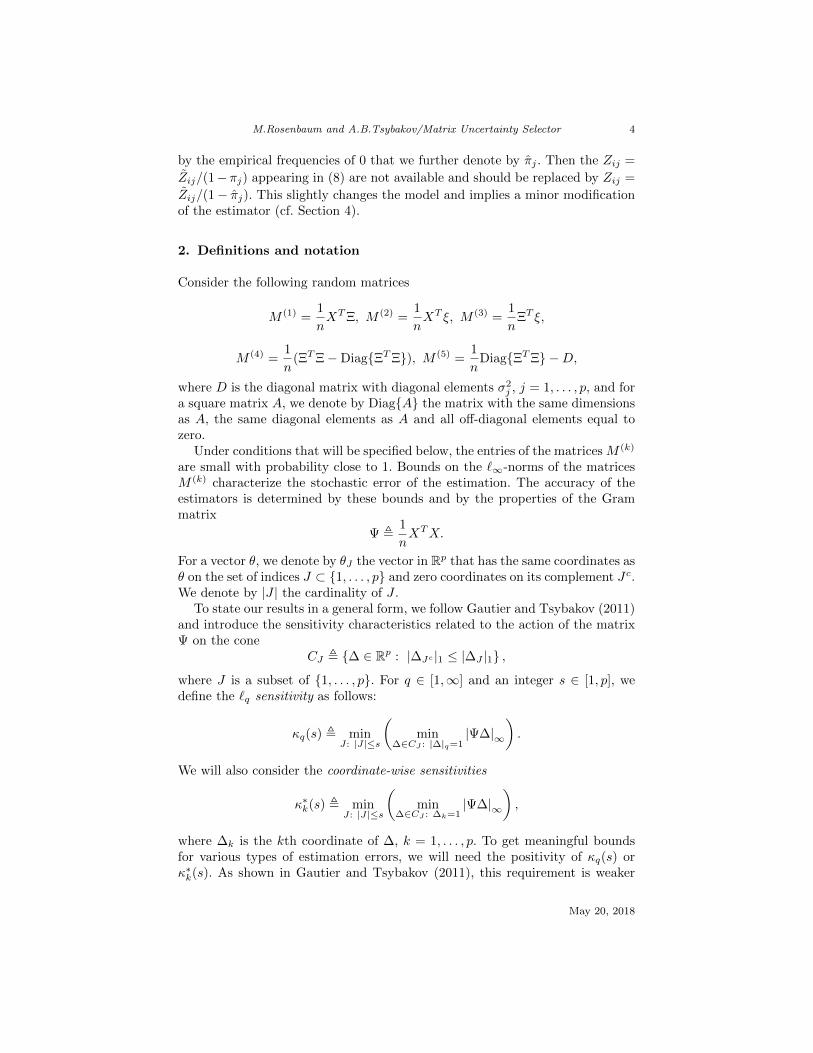
2. Definitions and notation
Consider the following random matrices
M (1) =1
nXTΞ, M (2) =
1
nXT ξ, M (3) =
1
nΞT ξ,
M (4) =1
n(ΞTΞ−Diag{ΞTΞ}), M (5) =
1
nDiag{ΞTΞ} −D,
where D is the diagonal matrix with diagonal elements σ2j , j = 1, . . . , p, and for
a square matrix A, we denote by Diag{A} the matrix with the same dimensionsas A, the same diagonal elements as A and all off-diagonal elements equal tozero.
Under conditions that will be specified below, the entries of the matrices M (k)
are small with probability close to 1. Bounds on the `∞-norms of the matricesM (k) characterize the stochastic error of the estimation. The accuracy of theestimators is determined by these bounds and by the properties of the Grammatrix
Ψ ,1
nXTX.
For a vector θ, we denote by θJ the vector in Rp that has the same coordinates asθ on the set of indices J ⊂ {1, . . . , p} and zero coordinates on its complement Jc.We denote by |J | the cardinality of J .
To state our results in a general form, we follow Gautier and Tsybakov (2011)and introduce the sensitivity characteristics related to the action of the matrixΨ on the cone
CJ , {∆ ∈ Rp : |∆Jc |1 ≤ |∆J |1} ,
where J is a subset of {1, . . . , p}. For q ∈ [1,∞] and an integer s ∈ [1, p], wedefine the `q sensitivity as follows:
κq(s) , minJ: |J|≤s
(min
∆∈CJ : |∆|q=1|Ψ∆|∞
).
We will also consider the coordinate-wise sensitivities
κ∗k(s) , minJ: |J|≤s
(min
∆∈CJ : ∆k=1|Ψ∆|∞
),
where ∆k is the kth coordinate of ∆, k = 1, . . . , p. To get meaningful boundsfor various types of estimation errors, we will need the positivity of κq(s) orκ∗k(s). As shown in Gautier and Tsybakov (2011), this requirement is weaker
May 20, 2018

M.Rosenbaum and A.B.Tsybakov/Matrix Uncertainty Selector 5
than the usual assumptions related to the structure of the Gram matrix Ψ, suchas the Restricted Eigenvalue assumption and the Coherence assumption. Forcompleteness, we recall these two assumptions.
Assumption RE(s). Let 1 ≤ s ≤ p. There exists a constant κRE(s) > 0such that
min∆∈CJ\{0}
|∆TΨ∆||∆J |22
≥ κRE(s)
for all subsets J of {1, . . . , p} of cardinality |J | ≤ s.
Assumption C. All the diagonal elements of Ψ are equal to 1 and all itsoff-diagonal elements of Ψij satisfy the coherence condition: maxi 6=j |Ψij | ≤ ρfor some ρ < 1.
Note that Assumption C with ρ < (3s)−1 implies Assumption RE(s) withκRE(s) =
√1− 3ρs, see Bickel et al. (2009) or Lemma 2 in Lounici (2008). From
Proposition 4.2 of Gautier and Tsybakov (2011) we get that, under AssumptionC with ρ < (2s)−1,
κ∞(s) ≥ 1− 2ρs, (10)
which yields the control of the sensitivities κq(s) for all 1 ≤ q ≤ ∞ since
κq(s) ≥ (2s)−1/qκ∞(s), ∀ 1 ≤ q ≤ ∞, (11)
by Proposition 4.1 of Gautier and Tsybakov (2011). Furthermore, Proposi-tion 9.2 of Gautier and Tsybakov (2011) implies that, under Assumption RE(s),
κ1(s) ≥ (4s)−1κRE(s), (12)
and by Proposition 9.3 of that paper, under Assumption RE(2s) for any s ≤ p/2and any 1 < q ≤ 2, we have
κq(s) ≥ C(q)s−1/qκRE(2s), (13)
where C(q) = 2−1/q−1/2(1 + (q − 1)
−1/q )−1.
3. Main results
In this section, we give bounds on the estimation and prediction errors of theCompensated MU selector. For ε ≥ 0, we consider the thresholds b(ε) ≥ 0 andδi(ε) ≥ 0, i = 1, . . . , 5, such that
P(
maxj=1,...,p
|σ2j − σ2
j | ≥ b(ε))≤ ε, (14)
andP(|M (i)|∞ ≥ δi(ε)) ≤ ε, i = 1, . . . , 5. (15)
May 20, 2018
M.Rosenbaum and A.B.Tsybakov/Matrix Uncertainty Selector 6
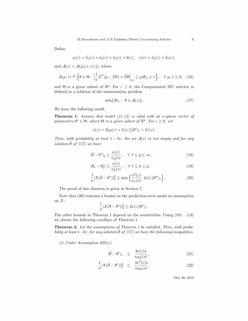
Define
µ(ε) = δ1(ε) + δ4(ε) + δ5(ε) + b(ε), τ(ε) = δ2(ε) + δ3(ε),
and A(ε) = A(µ(ε), τ(ε)), where
A(µ, τ) ,{θ ∈ Θ :
∣∣∣ 1nZT (y − Zθ) + Dθ
∣∣∣∞≤ µ|θ|1 + τ
}, ∀ µ, τ ≥ 0, (16)
and Θ is a given subset of Rp. For ε ≥ 0, the Compensated MU selector isdefined as a solution of the minimization problem
min{|θ|1 : θ ∈ A(ε)}, (17)
We have the following result.
Theorem 1. Assume that model (1)–(2) is valid with an s-sparse vector ofparameters θ∗ ∈ Θ, where Θ is a given subset of Rp. For ε ≥ 0, set
ν(ε) = 2(µ(ε) + δ1(ε)
)|θ∗|1 + 2τ(ε).
Then, with probability at least 1 − 6ε, the set A(ε) is not empty and for any
solution θ of (17) we have
|θ − θ∗|q ≤ν(ε)
κq(s), ∀ 1 ≤ q ≤ ∞, (18)
|θk − θ∗k| ≤ν(ε)
κ∗k(s), ∀ 1 ≤ k ≤ p, (19)
1
n|X(θ − θ∗)|22 ≤ min
{ν2(ε)
κ1(s), 2ν(ε)|θ∗|1
}. (20)
The proof of this theorem is given in Section 7.
Note that (20) contains a bound on the prediction error under no assumptionon X:
1
n|X(θ − θ∗)|22 ≤ 2ν(ε)|θ∗|1 .
The other bounds in Theorem 1 depend on the sensitivities. Using (10) – (13)we obtain the following corollary of Theorem 1.
Theorem 2. Let the assumptions of Theorem 1 be satisfied. Then, with proba-bility at least 1−6ε, for any solution θ of (17) we have the following inequalities.
(i) Under Assumption RE(s):
|θ − θ∗|1 ≤ 4ν(ε)s
κRE(s), (21)
1
n|X(θ − θ∗)|22 ≤ 4ν2(ε)s
κRE(s). (22)
May 20, 2018

M.Rosenbaum and A.B.Tsybakov/Matrix Uncertainty Selector 7
(ii) Under Assumption RE(2s), s ≤ p/2:
|θ − θ∗|q ≤ 4ν(ε)s1/q
κRE(2s), ∀ 1 < q ≤ 2. (23)
(iii) Under Assumption C with ρ < 12s :
|θ − θ∗|q <(2s)1/qν(ε)
1− 2ρs, ∀ 1 ≤ q ≤ ∞, (24)
where we set 1/∞ = 0.
If the components of ξ and Ξ are subgaussian, the values δi(ε) are of orderO(n−1/2) up to logarithmic factors, and the value b(ε) is of the same order in themodel with missing data (see Section 4). Then, the bounds for the CompensatedMU selector in Theorem 2 are decreasing with rate n−1/2 as n → ∞. This isan advantage of the Compensated MU selector as compared to the original MUselector θMU , for which the corresponding bounds do not decrease with n andcan be small only if the noise Ξ is small (cf. Rosenbaum and Tsybakov (2010)).
If the matrix X is observed without error (Ξ = 0), then µ(ε) = 0, δi(ε) =0, i 6= 2, and the Compensated MU selector coincides with the Dantzig selector.In this particular case, the results (ii) and (iii) of Theorem 2 improve, in terms ofthe constants or the range of validity, upon the corresponding bounds in Bickelet al. (2009) and Lounici (2008).
4. Control of the stochastic error terms
Theorems 1 and 2 are stated with general thresholds δi(ε) and b(ε), and can beused both for random or deterministic noises ξ,Ξ (in the latter case, ε = 0) andrandom or deterministic X. In this section, considering ε > 0 we first derivethe values δi(ε) for random ξ and Ξ with subgaussian entries, and then we
specify b(ε) and the matrix D for the model with missing data. Note that, forrandom ξ and Ξ, the values δi(ε) and b(ε) characterize the stochastic error ofthe estimator.
4.1. Thresholds δi(ε) under subgaussian noise
Recall that a zero-mean random variable W is said to be γ-subgaussian (γ > 0)if, for all t ∈ R,
IE[exp(tW )] ≤ exp(γ2t2/2). (25)
In particular, ifW is a zero-mean gaussian or bounded random variable, it is sub-gaussian. A zero-mean random variable W will be called (γ, t0)-subexponentialif there exist γ > 0 and t0 > 0 such that
IE[exp(tW )] ≤ exp(γ2t2/2), ∀ |t| ≤ t0. (26)
May 20, 2018
M.Rosenbaum and A.B.Tsybakov/Matrix Uncertainty Selector 8
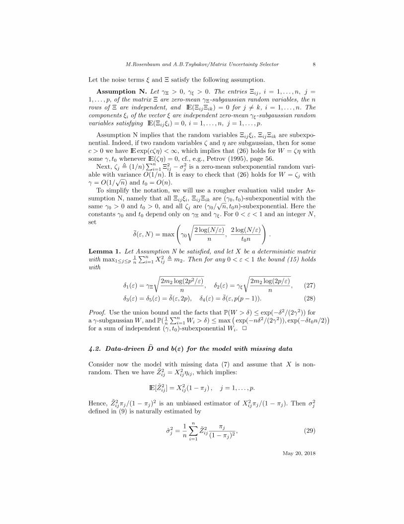
Let the noise terms ξ and Ξ satisfy the following assumption.
Assumption N. Let γΞ > 0, γξ > 0. The entries Ξij, i = 1, . . . , n, j =1, . . . , p, of the matrix Ξ are zero-mean γΞ-subgaussian random variables, the nrows of Ξ are independent, and IE(ΞijΞik) = 0 for j 6= k, i = 1, . . . , n. Thecomponents ξi of the vector ξ are independent zero-mean γξ-subgaussian randomvariables satisfying IE(Ξijξi) = 0, i = 1, . . . , n, j = 1, . . . , p.
Assumption N implies that the random variables Ξijξi, ΞijΞik are subexpo-nential. Indeed, if two random variables ζ and η are subgaussian, then for somec > 0 we have IE exp(cζη) <∞, which implies that (26) holds for W = ζη withsome γ, t0 whenever IE(ζη) = 0, cf., e.g., Petrov (1995), page 56.
Next, ζj , (1/n)∑ni=1 Ξ2
ij − σ2j is a zero-mean subexponential random vari-
able with variance O(1/n). It is easy to check that (26) holds for W = ζj withγ = O(1/
√n) and t0 = O(n).
To simplify the notation, we will use a rougher evaluation valid under As-sumption N, namely that all Ξijξi, ΞijΞik are (γ0, t0)-subexponential with thesame γ0 > 0 and t0 > 0, and all ζj are (γ0/
√n, t0n)-subexponential. Here the
constants γ0 and t0 depend only on γΞ and γξ. For 0 < ε < 1 and an integer N ,set
δ(ε,N) = max
(γ0
√2 log(N/ε)
n,
2 log(N/ε)
t0n
).
Lemma 1. Let Assumption N be satisfied, and let X be a deterministic matrixwith max1≤j≤p
1n
∑ni=1X
2ij , m2. Then for any 0 < ε < 1 the bound (15) holds
with
δ1(ε) = γΞ
√2m2 log(2p2/ε)
n, δ2(ε) = γξ
√2m2 log(2p/ε)
n, (27)
δ3(ε) = δ5(ε) = δ(ε, 2p), δ4(ε) = δ(ε, p(p− 1)). (28)
Proof. Use the union bound and the facts that P(W > δ) ≤ exp(−δ2/(2γ2)) fora γ-subgaussianW , and P( 1
n
∑ni=1Wi > δ) ≤ max
(exp(−nδ2/(2γ2)), exp(−δt0n/2)
)for a sum of independent (γ, t0)-subexponential Wi. 2
4.2. Data-driven D and b(ε) for the model with missing data
Consider now the model with missing data (7) and assume that X is non-random. Then we have Z2
ij = X2ijηij , which implies:
IE[Z2ij ] = X2
ij(1− πj) , j = 1, . . . , p.
Hence, Z2ijπj/(1 − πj)
2 is an unbiased estimator of X2ijπj/(1 − πj). Then σ2
j
defined in (9) is naturally estimated by
σ2j =
1
n
n∑i=1
Z2ij
πj(1− πj)2
, (29)
May 20, 2018

M.Rosenbaum and A.B.Tsybakov/Matrix Uncertainty Selector 9
The matrix D is then defined as a diagonal matrix with diagonal entries σ2j . It is
not hard to prove that σ2j approximates σ2
j in probability with rate O(n−1/2) upto a logarithmic factor. For example, let the probability that the data is missingbe the same for all j: π1 = · · · = πp , π∗. Then
P(|σ2j − σ2
j | ≥ b) = P
(∣∣∣∣∣ 1nn∑i=1
(Z2ij
π∗(1− π∗)2
−X2ij
π∗(1− π∗)
)∣∣∣∣∣ ≥ b)
= P
(∣∣∣∣∣ 1nn∑i=1
Z2ij −
X2ij
(1− π∗)
∣∣∣∣∣ ≥ b
π∗
)≤ 2 exp
(−2nb2(1− π∗)4
π2∗m4
),
where we have used the fact that 0 ≤ Z2ij ≤ X2
ij(1−π∗)−2, Hoeffding’s inequality
and the notation m4 , max1≤j≤p1n
∑ni=1X
4ij . This proves (14) with
b(ε) =π∗
(1− π∗)2
√m4 log(2p/ε)
2n.
If π∗ is unknown, we replace it by the estimator π = 1np
∑i,j 1{Zij=0}, where
1{·} denotes the indicator function. Another difference is that Zij = Zij/(1−πj)appearing in (8) are not available when πj ’s are unknown. Therefore, we slightly
modify the estimator using Zij instead of Zij ; we define θ as a solution of
min{|θ|1 : θ ∈ A(ε)} with
A(ε) ={θ ∈ Θ :
∣∣∣ 1nZT (y(1− π)− Zθ) + Dθ
∣∣∣∞≤ µ(ε)|θ|1 + τ(ε)
}, (30)
where µ(ε) and τ(ε) are suitably chosen constants, Z is the n × p matrix with
entries Zij , and D is a diagonal matrix with entries σ2j = 1
n
∑ni=1 Z
2ij π/(1− π)2.
This modification introduces in the bounds an additional term proportional toπ − π∗, which is of the order O((np)−1/2) in probability and hence is negligibleas compared to the error bound for the Compensated MU selector.
Remark 2. In this section, we have considered non-random X. Using the sameargument, it is easy to derive analogous expressions for σi(ε) and b(ε) whenX is a random matrix with independent sub-gaussian entries, and ξ, Ξ areindependent from X.
5. Confidence intervals
The bounds of Theorems 1 and 2 depend on the unknown matrix X via thesensitivities, and therefore cannot be used to provide confidence intervals. Inthis section, we show how to address the issue of confidence intervals by derivingother type of bounds based on the empirical sensitivities. Note first that thematrix Ψ = 1
nZTZ − D is a natural estimator of the unknown Gram matrix
Ψ. It is√n-consistent in `∞-norm under the conditions of the previous section.
May 20, 2018
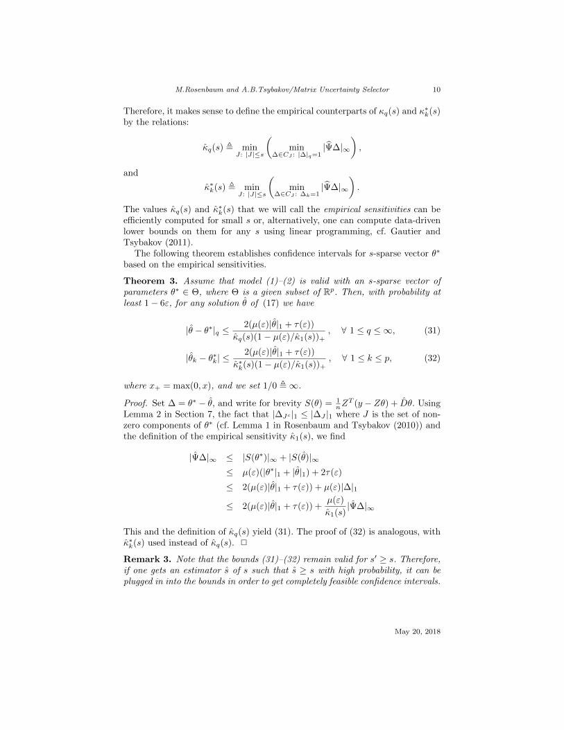
M.Rosenbaum and A.B.Tsybakov/Matrix Uncertainty Selector 10
Therefore, it makes sense to define the empirical counterparts of κq(s) and κ∗k(s)by the relations:
κq(s) , minJ: |J|≤s
(min
∆∈CJ : |∆|q=1|Ψ∆|∞
),
and
κ∗k(s) , minJ: |J|≤s
(min
∆∈CJ : ∆k=1|Ψ∆|∞
).
The values κq(s) and κ∗k(s) that we will call the empirical sensitivities can beefficiently computed for small s or, alternatively, one can compute data-drivenlower bounds on them for any s using linear programming, cf. Gautier andTsybakov (2011).
The following theorem establishes confidence intervals for s-sparse vector θ∗
based on the empirical sensitivities.
Theorem 3. Assume that model (1)–(2) is valid with an s-sparse vector ofparameters θ∗ ∈ Θ, where Θ is a given subset of Rp. Then, with probability atleast 1− 6ε, for any solution θ of (17) we have
|θ − θ∗|q ≤2(µ(ε)|θ|1 + τ(ε))
κq(s)(1− µ(ε)/κ1(s))+, ∀ 1 ≤ q ≤ ∞, (31)
|θk − θ∗k| ≤2(µ(ε)|θ|1 + τ(ε))
κ∗k(s)(1− µ(ε)/κ1(s))+, ∀ 1 ≤ k ≤ p, (32)
where x+ = max(0, x), and we set 1/0 ,∞.
Proof. Set ∆ = θ∗ − θ, and write for brevity S(θ) = 1nZ
T (y − Zθ) + Dθ. UsingLemma 2 in Section 7, the fact that |∆Jc |1 ≤ |∆J |1 where J is the set of non-zero components of θ∗ (cf. Lemma 1 in Rosenbaum and Tsybakov (2010)) andthe definition of the empirical sensitivity κ1(s), we find
|Ψ∆|∞ ≤ |S(θ∗)|∞ + |S(θ)|∞≤ µ(ε)(|θ∗|1 + |θ|1) + 2τ(ε)
≤ 2(µ(ε)|θ|1 + τ(ε)) + µ(ε)|∆|1
≤ 2(µ(ε)|θ|1 + τ(ε)) +µ(ε)
κ1(s)|Ψ∆|∞
This and the definition of κq(s) yield (31). The proof of (32) is analogous, withκ∗k(s) used instead of κq(s). 2
Remark 3. Note that the bounds (31)–(32) remain valid for s′ ≥ s. Therefore,if one gets an estimator s of s such that s ≥ s with high probability, it can beplugged in into the bounds in order to get completely feasible confidence intervals.
May 20, 2018
M.Rosenbaum and A.B.Tsybakov/Matrix Uncertainty Selector 11
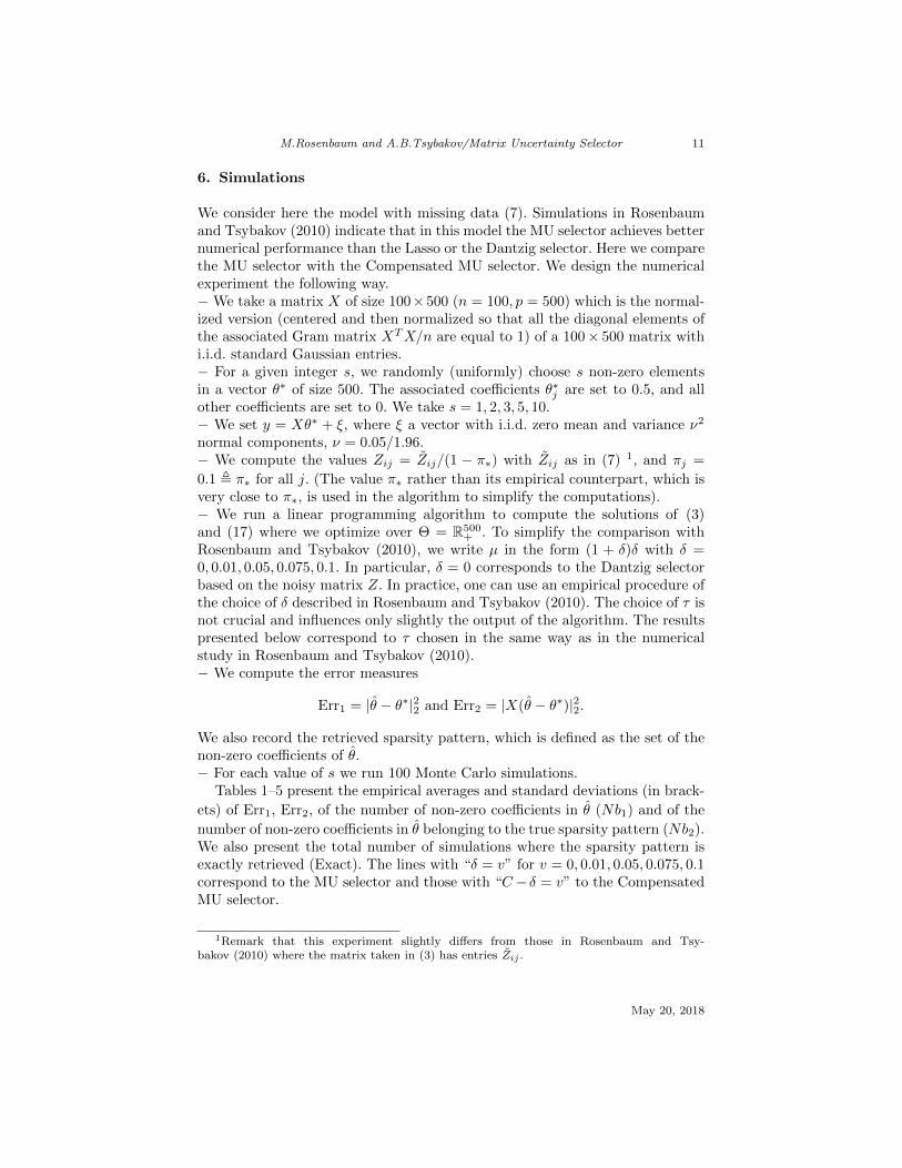
6. Simulations
We consider here the model with missing data (7). Simulations in Rosenbaumand Tsybakov (2010) indicate that in this model the MU selector achieves betternumerical performance than the Lasso or the Dantzig selector. Here we comparethe MU selector with the Compensated MU selector. We design the numericalexperiment the following way.−We take a matrix X of size 100×500 (n = 100, p = 500) which is the normal-ized version (centered and then normalized so that all the diagonal elements ofthe associated Gram matrix XTX/n are equal to 1) of a 100× 500 matrix withi.i.d. standard Gaussian entries.− For a given integer s, we randomly (uniformly) choose s non-zero elementsin a vector θ∗ of size 500. The associated coefficients θ∗j are set to 0.5, and allother coefficients are set to 0. We take s = 1, 2, 3, 5, 10.− We set y = Xθ∗ + ξ, where ξ a vector with i.i.d. zero mean and variance ν2
normal components, ν = 0.05/1.96.− We compute the values Zij = Zij/(1 − π∗) with Zij as in (7) 1, and πj =
0.1 , π∗ for all j. (The value π∗ rather than its empirical counterpart, which isvery close to π∗, is used in the algorithm to simplify the computations).− We run a linear programming algorithm to compute the solutions of (3)and (17) where we optimize over Θ = R500
+ . To simplify the comparison withRosenbaum and Tsybakov (2010), we write µ in the form (1 + δ)δ with δ =0, 0.01, 0.05, 0.075, 0.1. In particular, δ = 0 corresponds to the Dantzig selectorbased on the noisy matrix Z. In practice, one can use an empirical procedure ofthe choice of δ described in Rosenbaum and Tsybakov (2010). The choice of τ isnot crucial and influences only slightly the output of the algorithm. The resultspresented below correspond to τ chosen in the same way as in the numericalstudy in Rosenbaum and Tsybakov (2010).− We compute the error measures
Err1 = |θ − θ∗|22 and Err2 = |X(θ − θ∗)|22.
We also record the retrieved sparsity pattern, which is defined as the set of thenon-zero coefficients of θ.− For each value of s we run 100 Monte Carlo simulations.
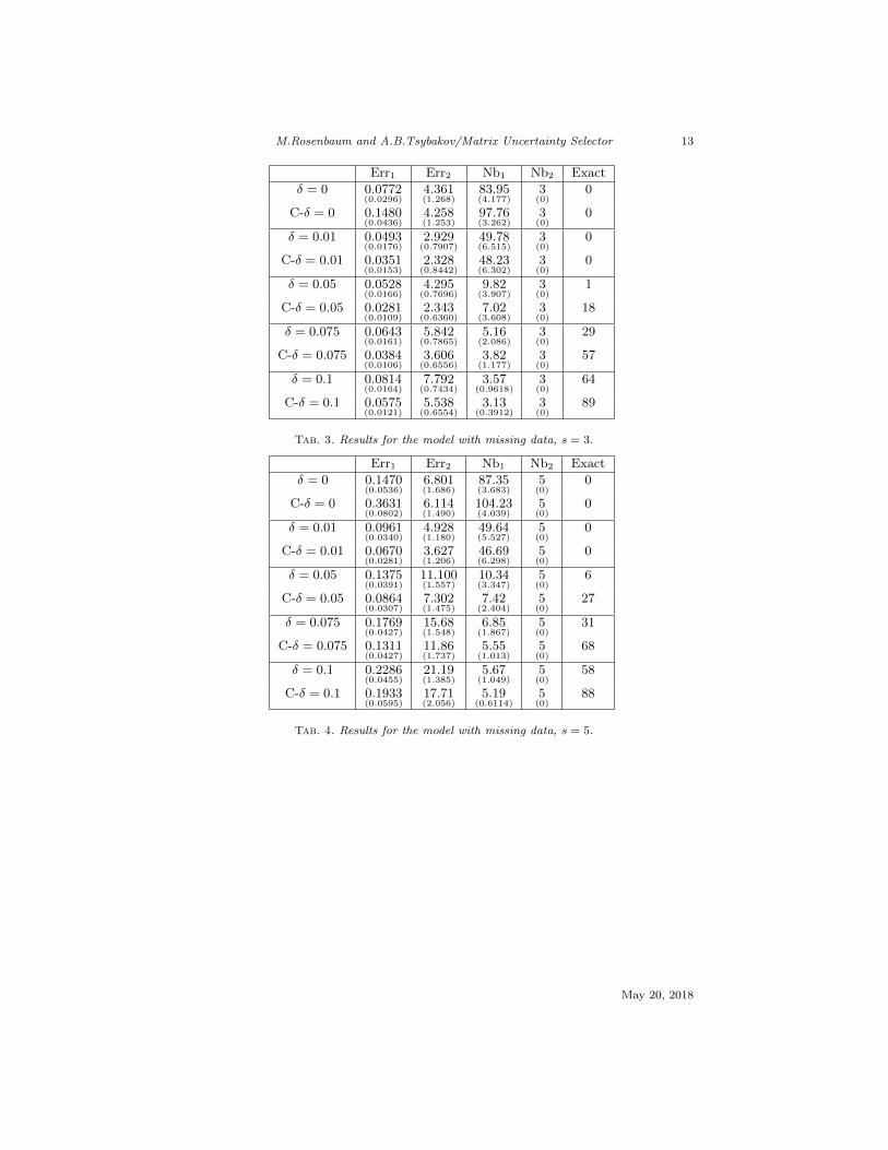
Tables 1–5 present the empirical averages and standard deviations (in brack-
ets) of Err1, Err2, of the number of non-zero coefficients in θ (Nb1) and of the
number of non-zero coefficients in θ belonging to the true sparsity pattern (Nb2).We also present the total number of simulations where the sparsity pattern isexactly retrieved (Exact). The lines with “δ = v” for v = 0, 0.01, 0.05, 0.075, 0.1correspond to the MU selector and those with “C− δ = v” to the CompensatedMU selector.
1Remark that this experiment slightly differs from those in Rosenbaum and Tsy-bakov (2010) where the matrix taken in (3) has entries Zij .
May 20, 2018

M.Rosenbaum and A.B.Tsybakov/Matrix Uncertainty Selector 12
Err1 Err2 Nb1 Nb2 Exact
δ = 0 0.0196(0.0114)
1.334(0.5865)
70.13(10.91)
1(0)
0
C-δ = 0 0.0225(0.0145)
1.495(0.6993)
80.09(8.343)
1(0)
0
δ = 0.01 0.0131(0.0069)
0.9318(0.3606)
45.45(9.507)
1(0)
1
C-δ = 0.01 0.0095(0.0062)
0.8386(0.4625)
46.88(9.737)
1(0)
0
δ = 0.05 0.0100(0.0038)
0.8001(0.2121)
12.45(5.798)
1(0)
3
C-δ = 0.05 0.0042(0.0027)
0.3412(0.1844)
10.52(5.764)
1(0)
6
δ = 0.075 0.0100(0.0030)
0.8878(0.1869)
6.28(4.261)
1(0)
14
C-δ = 0.075 0.0038(0.0020)
0.3377(0.1348)
4.91(3.674)
1(0)
21
δ = 0.1 0.0110(0.0024)
1.038(0.1582)
3.22(2.640)
1(0)
36
C-δ = 0.1 0.0044(0.0015)
0.4255(0.1040)
2.37(2.042)
1(0)
54
Tab. 1. Results for the model with missing data, s = 1.
Err1 Err2 Nb1 Nb2 Exact
δ = 0 0.0437(0.0170)
2.756(1.060)
80.04(5.149)
2(0)
0
C-δ = 0 0.0685(0.0275)
2.951(1.129)
92.67(3.911)
2(0)
0
δ = 0.01 0.0287(0.0107)
1.838(0.5423)
49.29(6.717)
2(0)
0
C-δ = 0.01 0.0201(0.0098)
1.561(0.6827)
48.18(6.775)
2(0)
0
δ = 0.05 0.0264(0.0093)
2.105(0.4960)
10.35(4.631)
2(0)
1
C-δ = 0.05 0.0125(0.0066)
0.9796(0.3849)
7.70(4.092)
2(0)
8
δ = 0.075 0.0301(0.0090)
2.694(0.5022)
4.77(2.587)
2(0)
24
C-δ = 0.075 0.0148(0.0052)
1.359(0.3573)
3.41(1.924)
2(0)
47
δ = 0.1 0.0371(0.0086)
3.521(0.4730)
2.62(1.046)
2(0)
65
C-δ = 0.1 0.0218(0.0059)
2.088(0.3853)
2.28(0.617)
2(0)
77
Tab. 2. Results for the model with missing data, s = 2.
May 20, 2018
M.Rosenbaum and A.B.Tsybakov/Matrix Uncertainty Selector 13
Err1 Err2 Nb1 Nb2 Exact
δ = 0 0.0772(0.0296)
4.361(1.268)
83.95(4.177)
3(0)
0
C-δ = 0 0.1480(0.0436)
4.258(1.253)
97.76(3.262)
3(0)
0
δ = 0.01 0.0493(0.0176)
2.929(0.7907)
49.78(6.515)
3(0)
0
C-δ = 0.01 0.0351(0.0153)
2.328(0.8442)
48.23(6.302)
3(0)
0
δ = 0.05 0.0528(0.0166)
4.295(0.7696)
9.82(3.907)
3(0)
1
C-δ = 0.05 0.0281(0.0109)
2.343(0.6360)
7.02(3.608)
3(0)
18
δ = 0.075 0.0643(0.0161)
5.842(0.7865)
5.16(2.086)
3(0)
29
C-δ = 0.075 0.0384(0.0106)
3.606(0.6556)
3.82(1.177)
3(0)
57
δ = 0.1 0.0814(0.0164)
7.792(0.7434)
3.57(0.9618)
3(0)
64
C-δ = 0.1 0.0575(0.0121)
5.538(0.6554)
3.13(0.3912)
3(0)
89
Tab. 3. Results for the model with missing data, s = 3.
Err1 Err2 Nb1 Nb2 Exact
δ = 0 0.1470(0.0536)
6.801(1.686)
87.35(3.683)
5(0)
0
C-δ = 0 0.3631(0.0802)
6.114(1.490)
104.23(4.039)
5(0)
0
δ = 0.01 0.0961(0.0340)
4.928(1.180)
49.64(5.527)
5(0)
0
C-δ = 0.01 0.0670(0.0281)
3.627(1.206)
46.69(6.298)
5(0)
0
δ = 0.05 0.1375(0.0391)
11.100(1.557)
10.34(3.347)
5(0)
6
C-δ = 0.05 0.0864(0.0307)
7.302(1.475)
7.42(2.404)
5(0)
27
δ = 0.075 0.1769(0.0427)
15.68(1.548)
6.85(1.867)
5(0)
31
C-δ = 0.075 0.1311(0.0427)
11.86(1.737)
5.55(1.013)
5(0)
68
δ = 0.1 0.2286(0.0455)
21.19(1.385)
5.67(1.049)
5(0)
58
C-δ = 0.1 0.1933(0.0595)
17.71(2.056)
5.19(0.6114)
5(0)
88
Tab. 4. Results for the model with missing data, s = 5.
May 20, 2018
M.Rosenbaum and A.B.Tsybakov/Matrix Uncertainty Selector 14
Err1 Err2 Nb1 Nb2 Exact
δ = 0 0.4479(0.1407)
14.56(3.060)
92.21(2.881)
10(0)
0
C-δ = 0 1.208(0.1705)
11.90(2.197)
117.23(6.532)
10(0)
0
δ = 0.01 0.3512(0.1263)
13.59(1.997)
52.76(5.340)
10(0)
0
C-δ = 0.01 0.2921(0.1317)
10.70(2.049)
48.74(6.067)
10(0)
0
δ = 0.05 0.7660(0.2395)
47.13(4.389)
20.29(4.152)
9.96(0.1959)
0
C-δ = 0.05 0.6919(0.2696)
41.55(5.709)
16.99(4.241)
9.94(0.2374)
1
δ = 0.075 0.9683(0.2721)
65.24(5.496)
16.78(3.545)
9.85(0.4092)
0
C-δ = 0.075 0.9443(0.3067)
61.23(7.066)
15.00(3.452)
9.76(0.5499)
5
δ = 0.1 1.150(0.2807)
82.86(6.745)
14.84(2.948)
9.58(0.6508)
1
C-δ = 0.1 1.157(0.3049)
80.43(8.359)
13.57(2.804)
9.39(0.7601)
11
Tab. 5. Results for the model with missing data, s = 10.
The results of the simulations are quite convincing. Indeed, the CompensatedMU selector improves upon the MU selector with respect to all the consideredcriteria, in particular when θ∗ is very sparse (s = 1, 2, 3). The order of magnitudeof the improvement is such that, for the best δ, the errors Err1 and Err2 aredivided by 2. The improvement is not so significant for larger s, especially fors = 10 when the model starts to be not very sparse. For all the values of s, thenon-zero coefficients of θ∗ are systematically in the sparsity pattern both of theMU selector and of the Compensated MU selector. The total number of non-zerocoefficients is always smaller (i.e., closer to the correct one) for the CompensatedMU selector. Finally, note that the best results for the error measures Err1 andErr2 are obtained with δ ≤ 0.075, while the sparsity pattern is better retrievedfor δ = 0.1. This reflects a trade-off between estimation and selection.
7. Proofs
Proof of Remark 1. It is enough to show that A(µ, τ) = B(µ, τ) where
B(µ, τ) = {θ ∈ Θ : ∃ u ∈ Rp such that (θ, u) ∈W (µ, τ)}.
Let first (θ, u) ∈ W (µ, τ). Using the triangle inequality, we easily get that θ ∈A(µ, τ). Now take θ ∈ A(µ, τ). We set
N =1
nZT (y − Zθ) + Dθ
and consider u ∈ Rp defined by
ui = −Ni1{|Ni|≤µ|θ|1} − sign(Ni)µ|θ|11{|Ni|>µ|θ|1},
for i = 1, . . . , p, where ui and Ni are the ith components of u and N respectively.It is easy to check that (θ, u) ∈W
(µ, τ
), which concludes the proof.
May 20, 2018
M.Rosenbaum and A.B.Tsybakov/Matrix Uncertainty Selector 15
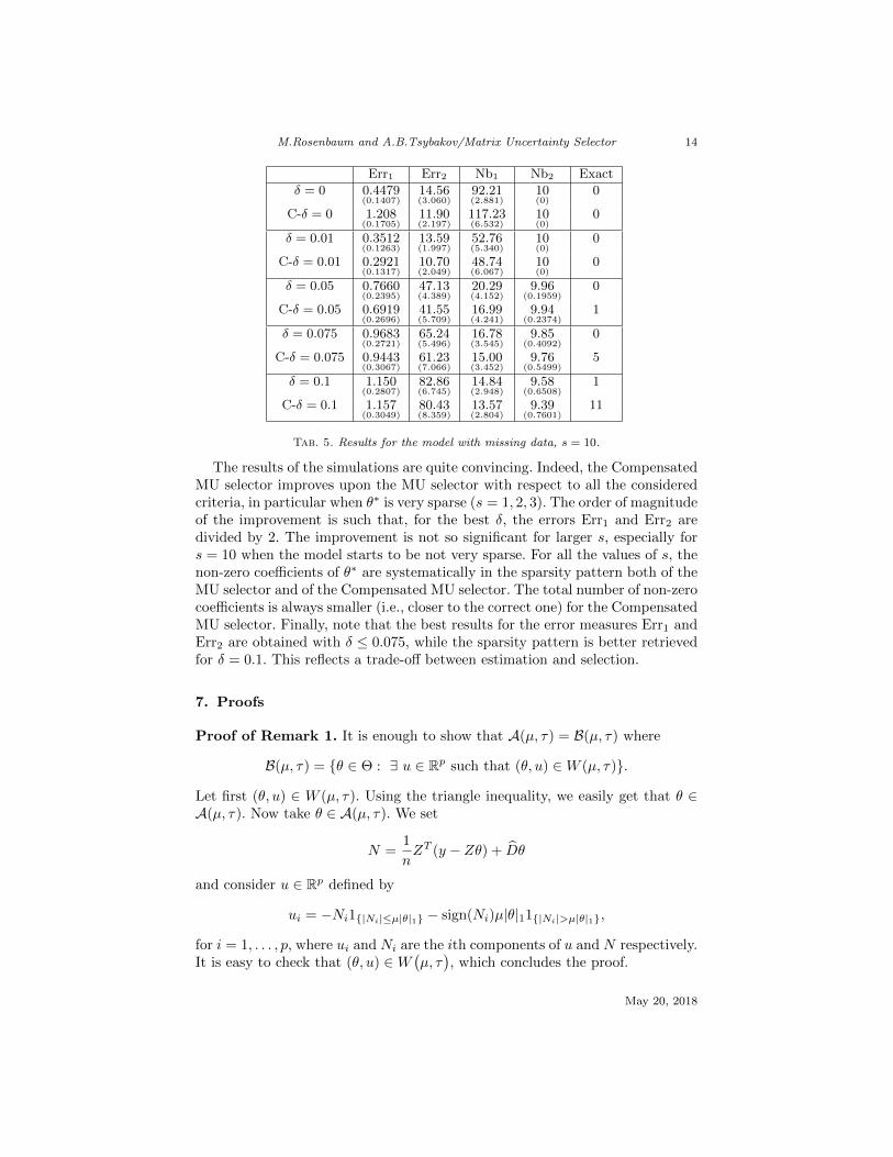
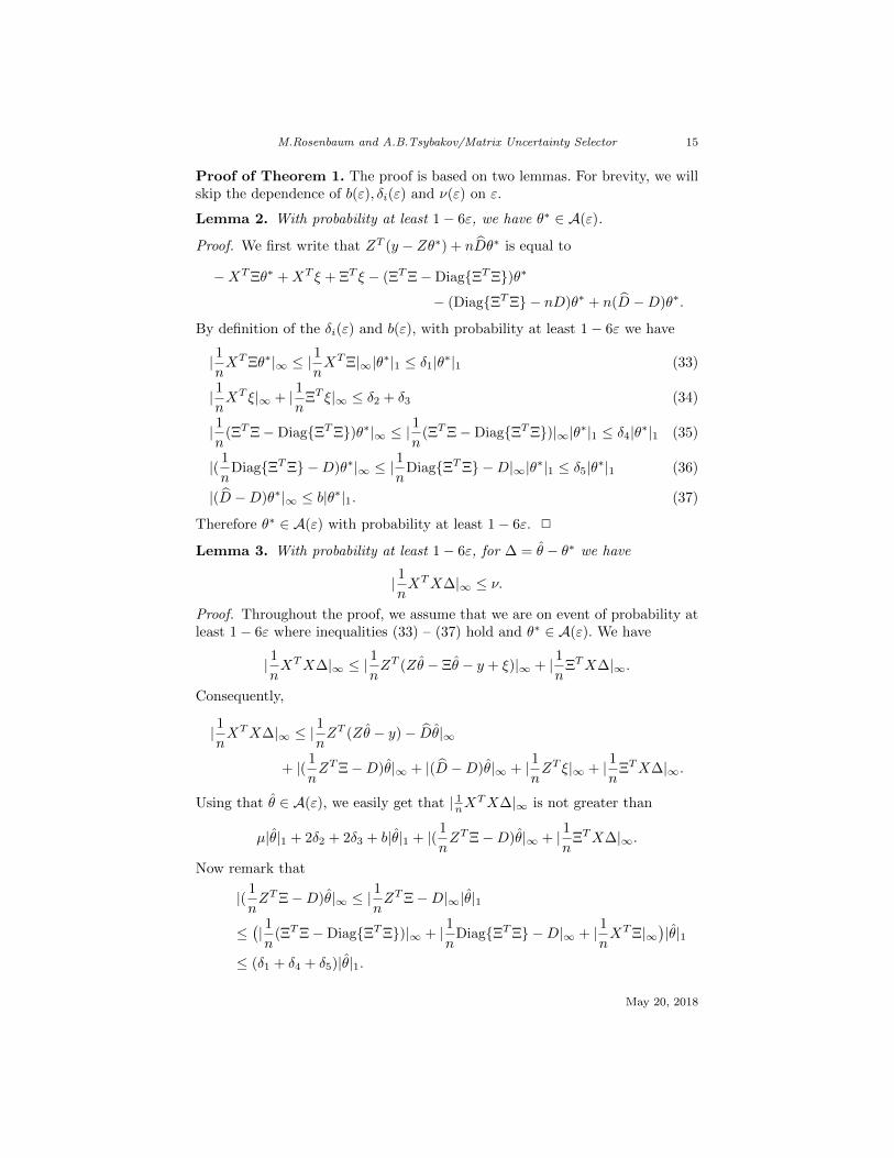
Proof of Theorem 1. The proof is based on two lemmas. For brevity, we willskip the dependence of b(ε), δi(ε) and ν(ε) on ε.
Lemma 2. With probability at least 1− 6ε, we have θ∗ ∈ A(ε).
Proof. We first write that ZT (y − Zθ∗) + nDθ∗ is equal to
−XTΞθ∗ +XT ξ + ΞT ξ − (ΞTΞ−Diag{ΞTΞ})θ∗
− (Diag{ΞTΞ} − nD)θ∗ + n(D −D)θ∗.
By definition of the δi(ε) and b(ε), with probability at least 1− 6ε we have
| 1nXTΞθ∗|∞ ≤ |
1
nXTΞ|∞|θ∗|1 ≤ δ1|θ∗|1 (33)
| 1nXT ξ|∞ + | 1
nΞT ξ|∞ ≤ δ2 + δ3 (34)
| 1n
(ΞTΞ−Diag{ΞTΞ})θ∗|∞ ≤ |1
n(ΞTΞ−Diag{ΞTΞ})|∞|θ∗|1 ≤ δ4|θ∗|1 (35)
|( 1
nDiag{ΞTΞ} −D)θ∗|∞ ≤ |
1
nDiag{ΞTΞ} −D|∞|θ∗|1 ≤ δ5|θ∗|1 (36)
|(D −D)θ∗|∞ ≤ b|θ∗|1. (37)
Therefore θ∗ ∈ A(ε) with probability at least 1− 6ε. 2
Lemma 3. With probability at least 1− 6ε, for ∆ = θ − θ∗ we have
| 1nXTX∆|∞ ≤ ν.
Proof. Throughout the proof, we assume that we are on event of probability atleast 1− 6ε where inequalities (33) – (37) hold and θ∗ ∈ A(ε). We have
| 1nXTX∆|∞ ≤ |
1
nZT (Zθ − Ξθ − y + ξ)|∞ + | 1
nΞTX∆|∞.
Consequently,
| 1nXTX∆|∞ ≤ |
1
nZT (Zθ − y)− Dθ|∞
+ |( 1
nZTΞ−D)θ|∞ + |(D −D)θ|∞ + | 1
nZT ξ|∞ + | 1
nΞTX∆|∞.
Using that θ ∈ A(ε), we easily get that | 1nXTX∆|∞ is not greater than
µ|θ|1 + 2δ2 + 2δ3 + b|θ|1 + |( 1
nZTΞ−D)θ|∞ + | 1
nΞTX∆|∞.
Now remark that
|( 1
nZTΞ−D)θ|∞ ≤ |
1
nZTΞ−D|∞|θ|1
≤(| 1n
(ΞTΞ−Diag{ΞTΞ})|∞ + | 1n
Diag{ΞTΞ} −D|∞ + | 1nXTΞ|∞
)|θ|1
≤ (δ1 + δ4 + δ5)|θ|1.
May 20, 2018
M.Rosenbaum and A.B.Tsybakov/Matrix Uncertainty Selector 16
Finally, using that
| 1n
ΞTX∆|∞ ≤ |θ − θ∗|1|1
nXTΞ|∞ ≤ δ1(|θ|1 + |θ∗|1)
together with the fact that |θ|1 ≤ |θ∗|1, we obtain the result. 2
We now proceed to the proof of Theorem 1. The bounds (18) and (19) followfrom Lemma 3, the fact that |∆Jc |1 ≤ |∆J |1 where J is the set of non-zerocomponents of θ∗ (cf. Lemma 1 in Rosenbaum and Tsybakov (2010)) and thedefinition of the sensitivities κq(s), κ
∗k(s). To prove (20), first note that
1
n|X∆|22 ≤
1
n|XTX∆|∞|∆|1, (38)
and use (18) with q = 1 and Lemma 3. This yields the first term under theminimum on the right hand side of (20). The second term is obtained again
from (38), Lemma 3 and the inequality |∆|1 ≤ |θ|1 + |θ∗|1 ≤ 2|θ∗|1.
Proof of Theorem 2. The bounds (21) and (24) follow by combining (18) with(12) and with (10) – (11) respectively. Next, (22) follows from (20) and (12).Also, as an easy consequence of (18) and (13) with q = 2 we get
|θ − θ∗|2 ≤4ν(ε)s1/2
κRE(2s).
Finally, (23) follows from this inequality and (21) using the interpolation formula
|∆|qq ≤ |∆|2−q1 |∆|2(q−1)
2 for ∆ = θ − θ∗, and the fact that κRE(s) ≥ κRE(2s).
References
[1] Belloni, A., and Chernozhukov, V. (2011). High dimensional sparse econo-metric models: an introduction. In: Inverse Problems and High Dimen-sional Estimation, Stats in the Chateau 2009, Alquier, P., E. Gautier, andG. Stoltz, Eds., Lecture Notes in Statistics, 203 127–162, Springer, Berlin.
[2] Bickel, P.J., Ritov, Y. and Tsybakov, A.B. (2009). Simultaneous analysisof Lasso and Dantzig selector. The Annals of Statistics 37 1705-1732.
[3] Bunea, F., Tsybakov, A.B. and Wegkamp, M.H. (2007a). Aggregation forGaussian regression. The Annals of Statistics 35 1674-1697.
[4] Bunea, F., Tsybakov, A.B. and Wegkamp, M.H. (2007b). Sparsity oracleinequalities for the Lasso, Electronic Journal of Statistics 1 169-194.
[5] Buhlmann, P., and S. A. van de Geer (2011). Statistics for High-Dimensional Data. Springer, New-York.
[6] Candes, E.J. and Tao, T. (2007). The Dantzig selector: statistical estima-tion when p is much larger than n (with discussion). The Annals of Statistics35 2313-2404.
[7] Gautier, E. and Tsybakov, A.B (2011) High-dimensional instrumental vari-ables regression and confidence sets. arXiv:1105.2454
May 20, 2018
M.Rosenbaum and A.B.Tsybakov/Matrix Uncertainty Selector 17
[8] Lounici, K. (2008). Sup-norm convergence rate and sign concentration prop-erty of Lasso and Dantzig estimators. Electronic Journal of Statistics 290-102.
[9] Koltchinskii, V. (2009). Dantzig selector and sparsity oracle inequalities.Bernoulli 15 799-828.
[10] Koltchinskii, V. (2011). Oracle inequalities in empirical risk minimizationand sparse recovery problems. Ecole d’Ete de Probabilites de Saint-Flour2008. Lecture Notes in Mathematics, Vol. 2033.
[11] Petrov,V.V. (1995). Sums of Independent Random Variables. Oxford Uni-versity Press.
[12] Rosenbaum, M. and Tsybakov A.B. (2010). Sparse recovery under matrixuncertainty. The Annals of Statistics 38 2620–2651.
May 20, 2018