1

Cosmology with Supernovae:Lecture 1

Josh Frieman

I Jayme Tiomno School of Cosmology, Rio de Janeiro, Brazil

July 2010

Hoje

• I. Cosmology Review• II. Observables: Age, Distances• III. Type Ia Supernovae as Standardizable

Candles• IV. Discovery Evidence for Cosmic

Acceleration• V. Current Constraints on Dark Energy

2

Coming Attractions• VI. Fitting SN Ia Light Curves & Cosmology

in detail (MLCS, SALT, rise vs. fall times)• VII. Systematic Errors in SN Ia Distances• VIII. Host-galaxy correlations• IX. SN Ia Theoretical Modeling• X. SN IIp Distances• XI. Models for Cosmic Acceleration• XII. Testing models with Future Surveys:

Photometric classification, SN Photo-z’s, & cosmology

3

References• Reviews:

Frieman, Turner, Huterer, Ann. Rev. of Astron. Astrophys., 46, 385 (2008)

Copeland, Sami, Tsujikawa, Int. Jour. Mod. Phys., D15, 1753 (2006)

Caldwell & Kamionkowski, Ann. Rev. Nucl. Part. Phys. (2009)

Silvestri & Trodden, Rep. Prog. Phys. 72:096901 (2009)

Kirshner, astro-ph/0910.0257

4

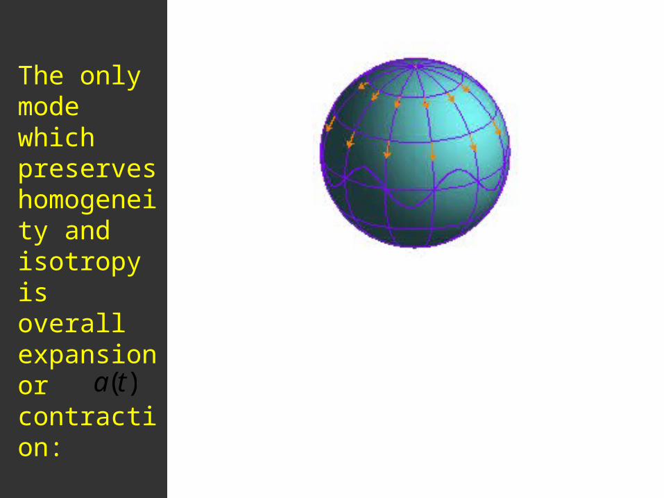
The only mode which preserves homogeneity and isotropy is overall expansion or contraction:

Cosmic scale factor

€

a(t)

6

On average, galaxies are at rest in these expanding(comoving) coordinates, and they are not expanding--they are gravitationally bound.

Wavelength of radiation scales with scale factor:

Redshift of light:

emitted at t1, observed at t2

€

a(t1)

€

a(t2)

€

λ ~ a(t)

€

1+ z =λ (t2)

λ (t1)=

a(t2)

a(t1)

7

Distance between galaxies:

where fixed comoving distance

Recession speed:

Hubble’s Law (1929)

€

a(t1)

€

a(t2)

€

υ =d(t2) − d(t1)

t2 − t1=

r[a(t2) − a(t1)]

t2 − t1

=d

a

da

dt≡ dH(t)

≈ dH0 for `small' t2 − t1

€

d(t) = a(t)r

€

r =

€

d(t2)

ModernHubbleDiagram Hubble Space TelescopeKeyProject

Freedman etal

Hubble parameter

Recent Measurement of H0

9

HST Distances to 240 Cepheid variable stars in 6 SN Ia host galaxies

Riess, etal 2009

€

H0 = 74.2 ± 3.6 km/sec/Mpc

How does the expansion of the Universe change over time?

Gravity:

everything in the Universe attracts everything else

expect the expansion of the Universe should slow

down over time

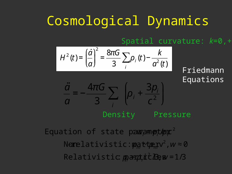
Cosmological Dynamics

€

˙ ̇ a

a= −

4πG

3 i

∑ ρ i +3pi

c 2

⎛

⎝ ⎜

⎞

⎠ ⎟

€

Equation of state parameter : wi = pi /ρ ic2

Non - relativistic matter : pm ~ ρ m v2, w ≈ 0

Relativistic particles : pr = ρ rc2 /3, w =1/3

€

H 2(t) =˙ a

a

⎛

⎝ ⎜

⎞

⎠ ⎟2

=8πG

3ρ i(t)

i

∑ −k

a2(t)FriedmannEquations

Density Pressure

Spatial curvature: k=0,+1,-1

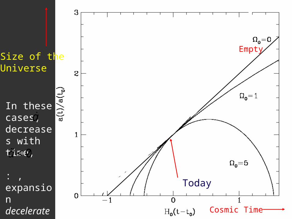
Size of theUniverse

Cosmic Time

Empty

Today

In these cases, decreases with time, : ,expansion decelerates

€

˙ a

€

˙ ̇ a < 0

Cosmological Dynamics

€

˙ ̇ a

a= −

4πG

3 i

∑ ρ i +3pi

c 2

⎛

⎝ ⎜

⎞

⎠ ⎟

€

Equation of state parameter : wi = pi /ρ ic2

Non - relativistic matter : pm ~ ρ m v2, w ≈ 0

Relativistic particles : pr = ρ rc2 /3, w =1/3

Dark Energy : component with negative pressure : wDE < −1/3

€

H 2(t) =˙ a

a

⎛

⎝ ⎜

⎞

⎠ ⎟2

=8πG

3ρ i(t)

i

∑ −k

a2(t)FriedmannEquations

Size of theUniverse

Cosmic Time

EmptyAccelerating

Today

p = (w = 1)

€

˙ ̇ a > 0

15

``Supernova Data”

16

Discovery of Cosmic Acceleration from High-redshiftSupernovae

Type Ia supernovae that exploded when the Universe was 2/3 its present size are ~25% fainter than expected

= 0.7 = 0.m = 1.

Log(distance)

redshift

Accelerating

Not accelerating

Cosmic Acceleration

This implies that increases with time: if we could watch the same galaxy over cosmic time, we would see its recession speed increase.

Exercise 1: A. Show that above statement is true. B. For a galaxy at d=100 Mpc, if H0=70 km/sec/Mpc =constant, what is the increase in its recession speed over a 10-year period? How feasible is it to measure that change?

€

˙ ̇ a > 0 →

˙ a = Ha increases with time

€

υ =Hd

Cosmic Acceleration

What can make the cosmic expansion speed up?

1. The Universe is filled with weird stuff that gives rise to `gravitational repulsion’. We call this Dark Energy

2. Einstein’s theory of General Relativity is wrong on cosmic distance scales.

3. We must drop the assumption of homogeneity/isotropy.

19

Cosmological Constant as Dark Energy

Einstein:

Zel’dovich and Lemaitre:

€

Gμν − Λgμν = 8πGTμν

Gμν = 8πGTμν + Λgμν

≡ 8πG Tμν (matter) + Tμν (vacuum)( )

€

Tμν (vac) =Λ

8πGgμν

ρ vac = T00 =Λ

8πG, pvac = Tii = −

Λ

8πG

wvac = −1 ⇒ H = constant ⇒ a(t)∝ exp(Ht)

Cosmological Constant as Dark Energy Quantum zero-point fluctuations: virtual particles continuously fluctuate into and out of the vacuum (via the Uncertainty principle).

Vacuum energy density in Quantum Field Theory:

Theory: Data:

Pauli

€

ρvac =Λ

8πG=

1

V

1

2h∑ ω = hc(k 2 + m2

0

M

∫ )1/ 2 d3k ~ M 4

wvac =pvac

ρ vac

= −1, ρ vac = const.

€

M ~ MPlanck = G−1/ 2 =1028 eV ⇒ ρ vac ~ 10112 eV4

ρ vac <10−10eV4

Cosmological Constant Problem

Components of the Universe

Dark Matter: clumps, holds galaxies and clusters togetherDark Energy: smoothly distributed, causes expansion of Universe to

speed up

€

ρm ~ a−3

€

ρr ~ a−4

€

ρDE ~ a−3(1+w )

€

wi(z) ≡pi

ρ i

˙ ρ i + 3Hρ i(1+ wi) = 0

=Log[a0/a(t)]

Equation of State parameter w determines Cosmic Evolution

Conservation of Energy-Momentum

23

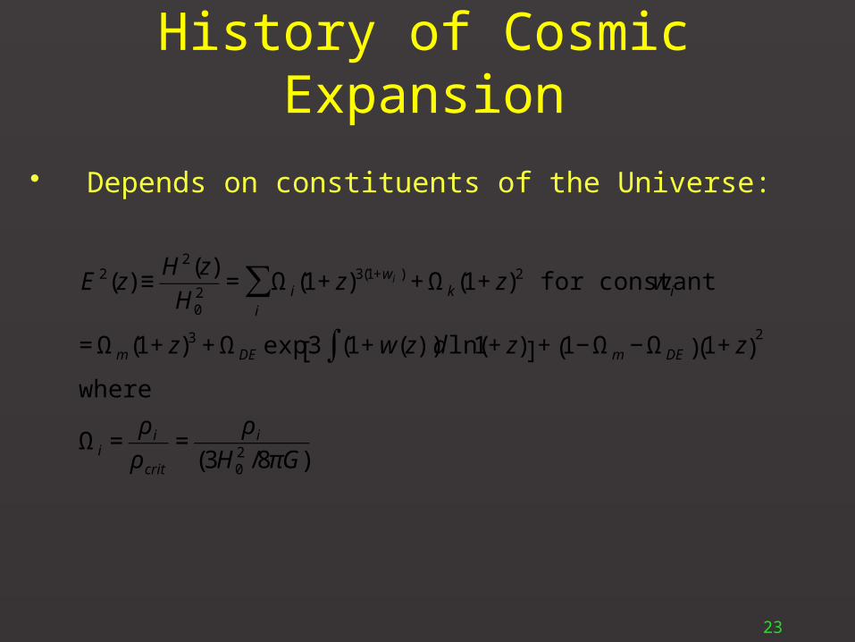
• Depends on constituents of the Universe:

History of Cosmic Expansion

€

E 2(z) ≡H 2(z)

H02

= Ω i

i

∑ (1+ z)3(1+wi ) + Ωk (1+ z)2 for constant wi

= Ωm (1+ z)3 + ΩDE exp 3 (1+ w(z))d ln(1+ z)∫[ ] + 1− Ωm − ΩDE( ) 1+ z( )2

where

Ω i =ρ i

ρ crit

=ρ i

(3H02 /8πG)

24

Cosmological Observables

€

ds2 = c 2dt 2 − a2(t) dχ 2 + Sk2(χ ) dθ 2 + sin2 θ dφ2

{ }[ ]

= c 2dt 2 − a2(t)dr2

1− kr2+ r2 dθ 2 + sin2 θ dφ2

{ } ⎡

⎣ ⎢

⎤

⎦ ⎥

Friedmann-Robertson-WalkerMetric:

where

Comoving distance:€

r = Sk (χ ) = sinh(χ ), χ , sin(χ ) for k = −1,0,1

€

cdt = a dχ ⇒ χ =cdt

a∫ =

cdt

ada∫ da = c

da

a2H(a)∫

€

a =1

1+ z ⇒ da = −(1+ z)−2 dz = −a2dz

cdt

dada = adχ ⇒ −

c˙ a

a2dz = adχ ⇒ − cdz = H(z)dχ

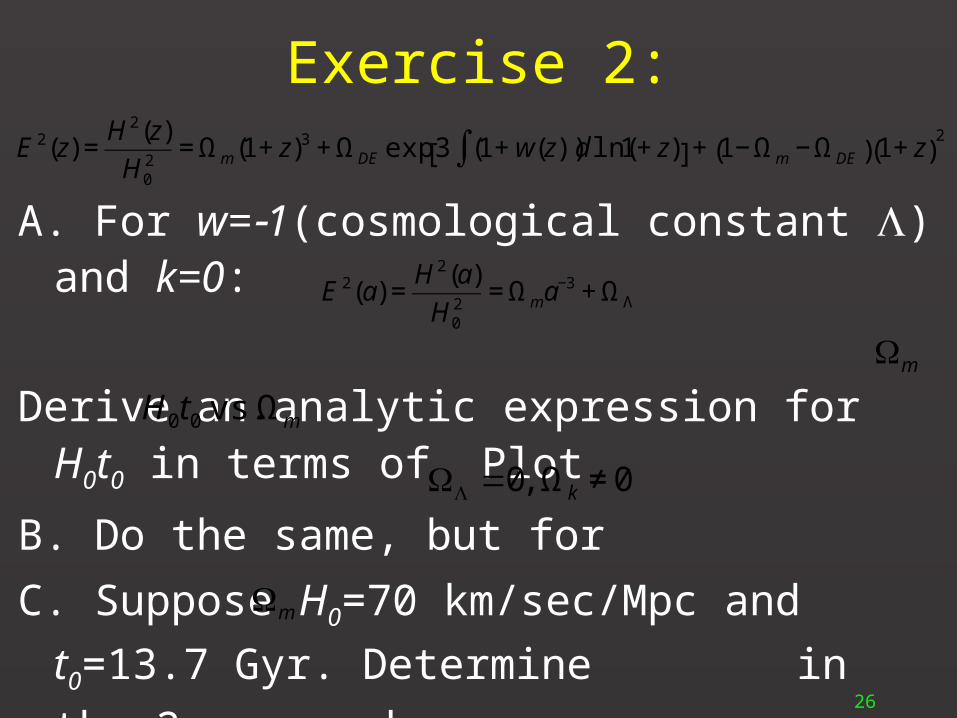
Age of the Universe

25

€

cdt = adχ

t = adχ =da

aH(a)∫∫ =

dz

(1+ z)H(z)∫

t0 =1

H0

dz

(1+ z)E(z)0

∞

∫

where E(z) = H(z) /H0

26

Exercise 2:

A. For w=1(cosmological constant ) and k=0:

Derive an analytic expression for H0t0 in terms of

Plot

B. Do the same, but for

C. Suppose H0=70 km/sec/Mpc and t0=13.7 Gyr.

Determine in the 2 cases above.

D. Repeat part C but with H0=72.

€

E 2(z) =H 2(z)

H02

= Ωm (1+ z)3 + ΩDE exp 3 (1+ w(z))d ln(1+ z)∫[ ] + 1− Ωm − ΩDE( ) 1+ z( )2

€

E 2(a) =H 2(a)

H02

= Ωma−3 + ΩΛ

€

Ωm

€

H0t0 vs. Ωm

€

ΩΛ =0, Ωk ≠ 0

€

Ωm

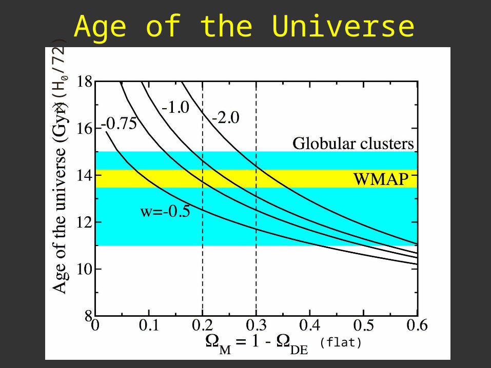
Age of the Universe(

H0/

72)

(flat)

Luminosity Distance• Source S at origin emits light at time t1 into solid angle d, received by observer O at coordinate distance r at time t0, with detector of area A:

S

A

r

Proper area of detector given by the metric:

Unit area detector at O subtends solid angle

at S.

Power emitted into d is

Energy flux received by O per unit area is

€

A = a0r dθ a0rsinθ dφ = a02r2dΩ

€

dΩ =1/a02r2

€

dP = L dΩ /4π

€

f =L dΩ

4π=

L

4πa02r2

Include Expansion

• Expansion reduces received flux due to 2 effects: 1. Photon energy redshifts:

2. Photons emitted at time intervals t1 arrive at time

intervals t0: €

Eγ (t0) = Eγ (t1) /(1+ z)

€

dt

a(t)t1

t0

∫ =dt

a(t)t1 +δ t1

t0 +δ t0

∫

dt

a(t)t1

t1 +δ t1

∫ +dt

a(t)t1 +δ t1

t0

∫ =dt

a(t)t1 +δ t1

t0

∫ +dt

a(t)t0

t0 +δ t0

∫

δt1a(t1)

=δt0

a(t0) ⇒

δt0

δt1=

a(t0)

a(t1)=1+ z

€

f =L dΩ

4π=

L

4πa02r2(1+ z)2

≡L

4πdL2

⇒ dL = a0r(1+ z) = (1+ z)2 dA

Luminosity DistanceConvention: choose a0=1

30

Worked Example I

For w=1(cosmological constant ):

Luminosity distance:

€

E 2(z) =H 2(z)

H02

= Ωm (1+ z)3 + ΩDE exp 3 (1+ w(z))d ln(1+ z)∫[ ] + 1− Ωm − ΩDE( ) 1+ z( )2

€

dL (z;Ωm,ΩΛ ) = r(1+ z) = c(1+ z)Sk

da

H0a2E(a)

∫ ⎛

⎝ ⎜

⎞

⎠ ⎟

= c(1+ z)Sk

da

H0a2[Ωma−3 + ΩΛ + (1− Ωm − ΩΛ )a−2]1/ 2∫

⎛

⎝ ⎜

⎞

⎠ ⎟

€

E 2(a) =H 2(a)

H02

= Ωma−3 + ΩΛ + 1− Ωm − ΩΛ( )a−2

31

Worked Example II

For a flat Universe (k=0) and constant Dark Energy equation of state w:

Luminosity distance:

€

E 2(z) =H 2(z)

H02

= Ωm (1+ z)3 + ΩDE exp 3 (1+ w(z))d ln(1+ z)∫[ ] + 1− Ωm − ΩDE( ) 1+ z( )2

€

E 2(z) =H 2(z)

H02

= (1− ΩDE )(1+ z)3 + ΩDE (1+ z)3(1+w )

€

dL (z;ΩDE ,w) = r(1+ z) = χ (1+ z) =c(1+ z)

H0

da

a2E(a)∫

=c(1+ z)

H0

1+ ΩDE[(1+ z)3w −1]−1/ 2

(1+ z)3 / 2∫ dz

Note: H0dL is independent of H0

32

Dark Energy Equation of State

Curves of

constant dL

at fixed z

z =

Flat Universe

Exercise 3

• Make the same plot for Worked Example I: plot curves of constant luminosity distance (for several choices of redshift between 0.1 and 1.0) in the plane of , choosing the distance for the model with as the fiducial.

• In the same plane, plot the boundary of the region between present acceleration and deceleration.

• Extra credit: in the same plane, plot the boundary of the region that expands forever vs. recollapses.

33

€

ΩΛvs. Ωm

€

ΩΛ = 0.7, Ωm = 0.3

34

Bolometric Distance Modulus• Logarithmic measures of luminosity and flux:

• Define distance modulus:

• For a population of standard candles (fixed M), measurements of vs. z, the Hubble diagram, constrain cosmological parameters.

€

M = −2.5log(L) + c1, m = −2.5log( f ) + c2

€

μ ≡m − M = 2.5log(L / f ) + c3 = 2.5log(4πdL2) + c3

= 5log[H0dL (z;Ωm,ΩDE ,w(z))]− 5log H0 + c4

flux measure redshift from spectra

Exercise 4

• Plot distance modulus vs redshift (z=0-1) for:• Flat model with• Flat model with• Open model with

– Plot first linear in z, then log z.

• Plot the residual of the first two models with respect to the third model

35

€

Ωm =1

€

ΩΛ =0.7, Ωm = 0.3

€

Ωm = 0.3

36

Discovery of Cosmic Acceleration from High-redshiftSupernovae

Type Ia supernovae that exploded when the Universe was 2/3 its present size are ~25% fainter than expected

= 0.7 = 0.m = 1.

Log(distance)

redshift

Accelerating

Not accelerating

37

Distance Modulus• Recall logarithmic measures of luminosity and flux:

• Define distance modulus:

• For a population of standard candles (fixed M) with known spectra (K) and known extinction (A), measurements of vs. z, the Hubble diagram, constrain cosmological parameters.

€

M i = −2.5log(Li) + c1, mi = −2.5log( f i) + c2

€

μ ≡mi − M j = 2.5log(L / f ) + K ij (z) + c3 = 2.5log(4πdL2) + K + c3

= 5log[H0dL (z;Ωm,ΩDE ,w(z))]− 5log H0 + K ij (z) + Ai + c4

denotes passband

38

K corrections due to redshiftSN spectrum

Rest-frame B band filter

Equivalent restframe i band filter at different redshifts

(iobs=7000-8500 A)

€

f i = Si(λ )Fobs(λ )dλ∫= (1+ z) Si∫ [λ rest (1+ z)]Frest (λ rest )dλ rest

39

Absolute vs. Relative Distances• Recall logarithmic measures of luminosity and flux:

• If Mi is known, from measurement of mi can infer absolute distance to

an object at redshift z, and thereby determine H0 (for z<<1, dL=cz/H0)

• If Mi (and H0) unknown but constant, from measurement of mi can

infer distance to object at redshift z1 relative to object at distance z2:

independent of H0

• Use low-redshift SNe to vertically `anchor’ the Hubble diagram, i.e., to determine

€

M i = −2.5log(Li) + c1, mi = −2.5log( f i) + c2

€

mi = 5log[H0dL ] − 5logH0 + M i + K(z) + c4

€

m1 − m2 = 5logd1

d2

⎛

⎝ ⎜

⎞

⎠ ⎟+ K1 − K2

€

M − 5logH0

40

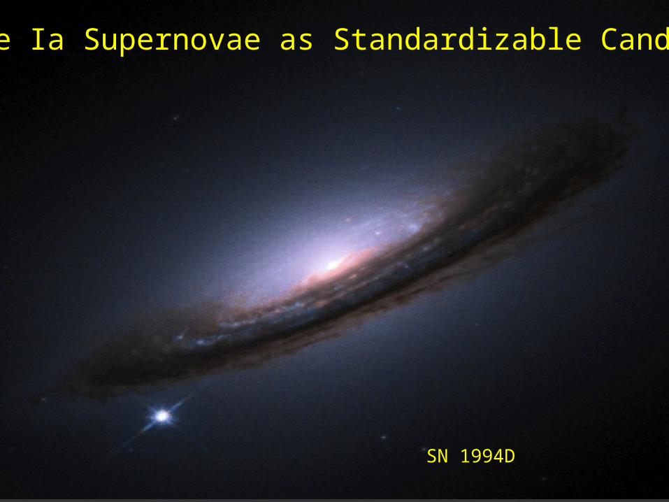
SN 1994D

Type Ia Supernovae as Standardizable Candles

41

42

SN Spectra

~1 week

after

maximum

light

Filippenko 1997

Ia

II

Ic

Ib

Type Ia SupernovaeThermonuclear explosions of Carbon-Oxygen White Dwarfs

White Dwarf accretes mass from or merges with a companion star, growing to a critical mass~1.4Msun

(Chandrasekhar)

After ~1000 years of slow cooking, a violent explosion is triggered at or near the center, and the star is completely incinerated within seconds

In the core of the star, light elements are burned in fusion reactions to form Nickel. The radioactive decay of Nickel and Cobalt makes it shine for a couple of months

44

Type Ia SupernovaeGeneral properties:

• Homogeneous class* of events, only small (correlated) variations• Rise time: ~ 15 – 20 days• Decay time: many months• Bright: MB ~ – 19.5 at peak

No hydrogen in the spectra• Early spectra: Si, Ca, Mg, ...(absorption)• Late spectra: Fe, Ni,…(emission)• Very high velocities (~10,000 km/s)

SN Ia found in all types of galaxies, including ellipticals• Progenitor systems must have long lifetimes

*luminosity, color,spectra at max. light

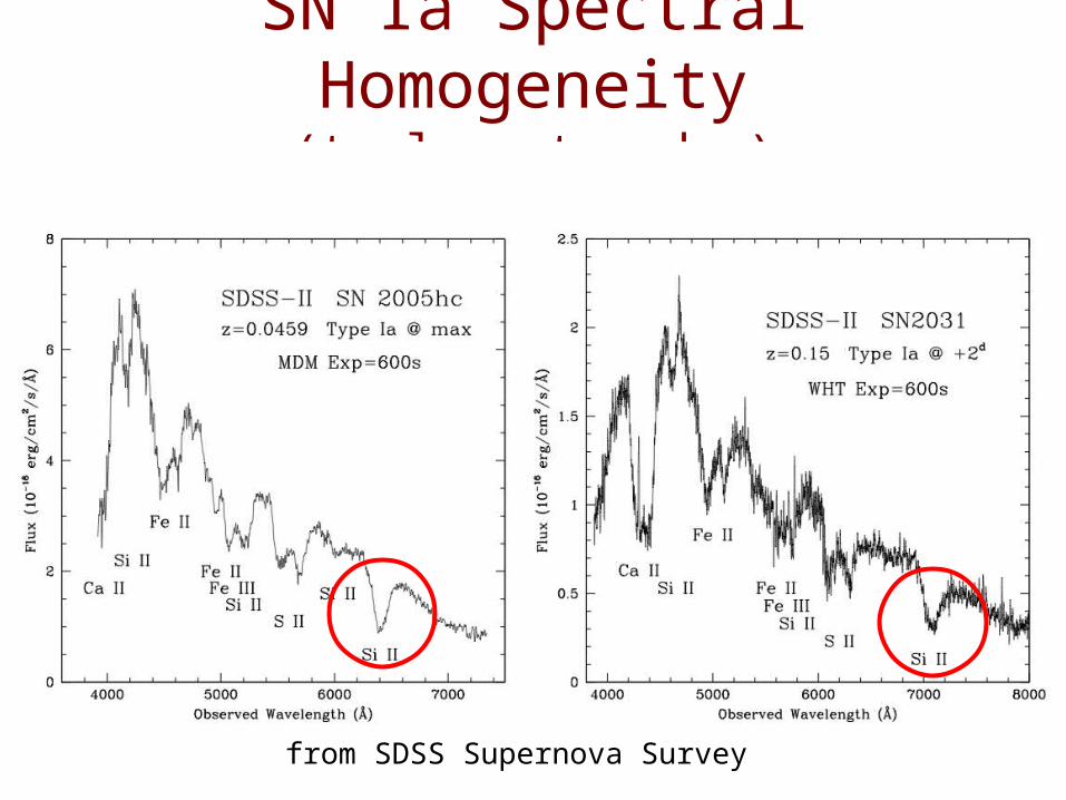
SN Ia Spectral Homogeneity(to lowest order)

from SDSS Supernova Survey

46

Spectral Homogeneity at fixed epoch

47

SN2004ar z = 0.06 from SDSS galaxy spectrum

Galaxy-subtracted

Spectrum

SN Ia

template

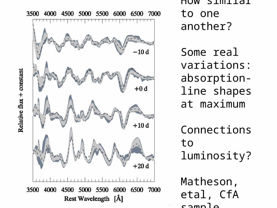
How similar to one another?

Some real variations: absorption-line shapes at maximum

Connections to luminosity?

Matheson, etal, CfA sample

49Hsiao etal

Supernova Ia Spectral Evolution

Late times

Early times

50

Layered

Chemical

Structure

provides

clues to

Explosion

physics

51

SDSS

Filter

Bandpasses€

S(λ )

52

Model

SN Ia Light Curves in SDSS filters synthesized from composite template spectral sequence

SNe evolve in time from blue to red;

K-corrections are time-dependent

€

mi = −2.5logSi(λ )F(λ )dλ∫

Si(λ )dλ∫+ Ζ i

53

SN1998bu Type Ia

Multi-band Light curve

Extremely few light-curves are this well sampled

Suntzeff, etal

Jha, etal

Hernandez, etal

Lum

inos

ity

Time

m15

15 days

Empirical Correlation: Brighter SNe Ia decline more slowly and are bluerPhillips 1993

SN Ia Peak LuminosityEmpirically correlatedwith Light-Curve Decline Rate

Brighter Slower

Use to reduce Peak Luminosity Dispersion

Phillips 1993

Pea

k L

umin

osit

y

Rate of declineGarnavich, etal

56

Type Ia SNPeak Brightnessas calibratedStandard Candle

Peak brightnesscorrelates with decline rate

Variety of algorithms for modeling these correlations: corrected dist. modulus

After correction,~ 0.16 mag(~8% distance error)

Lum

inos

ity

Time

57

Published Light Curves for Nearby Supernovae

Low-z SNe:

Anchor Hubble diagram

Train Light-curve fitters

Need well-sampled, well-calibrated, multi-band light curves

58

Carnegie

Supernova

Project

Nearby

Optical+

NIR LCs

59

Correction for Brightness-Decline relation reduces scatter in nearby SN Ia Hubble Diagram

Distance modulus for z<<1:

Corrected distance modulus is not a direct observable: estimated from a model for light-curve shape

€

m − M = 5logυ − 5log H0

Riess etal 1996

60

Acceleration Discovery Data:High-z SN Team

10 of 16 shown; transformed to SN rest-frame

Riess etal

Schmidt etal

V

B+1

61

Discovery of Cosmic Acceleration from High-redshiftSupernovae

Apply same brightness-decline relation at high z

Type Ia supernovae that exploded when the Universe was 2/3 its present size are ~25% fainter than expected

= 0.7 = 0.m = 1.

Log(distance)

redshift

Accelerating

Not accelerating

HZTSCP

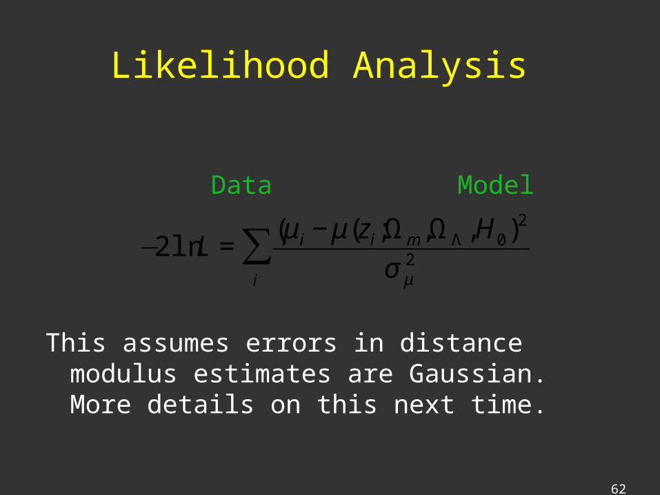
Likelihood Analysis

This assumes errors in distance modulus estimates are Gaussian. More details on this next time.

62

€

−2ln L =(μ i − μ(zi;Ωm,ΩΛ ,H0)2

σ μ2

i

∑

Data Model

63

Exercise 5

• Carry out a likelihood analysis of using the High-Z Supernova Data of Riess, etal 1998: see following tables. Assume a fixed Hubble parameter for this exercise.

• Extra credit: marginalize over H0 with a flat prior.

64

€

ΩΛ , Ωm

Riess, etal High-z Data (1998)

65

Low-z Data

66