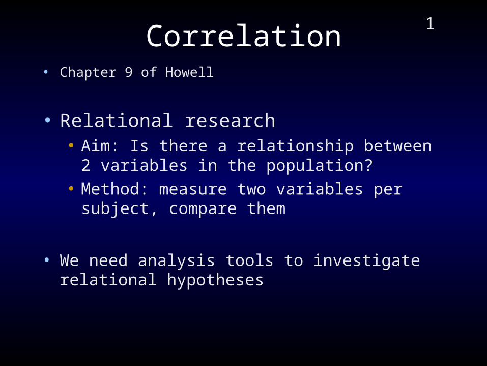
1Correlation

• Chapter 9 of Howell

• Relational research• Aim: Is there a relationship between 2 variables in the

population?

• Method: measure two variables per subject, compare them

• We need analysis tools to investigate relational hypotheses

2Looking for relationships

• How do we decide if two variables are “related”• What is a relationship?

• Think of things that are related• Rain and cold (always happen together)

• learning and performance

• What do these have in common?

3Related variables

• Rain and cold• the colder it gets, the more it rains OR

• the lower the temperature, the more it rains

• Learning and performance• the more you learn, the better you perform

OR

• the higher the learning, the higher the performance

4

Working with two variables

• Imagining 2 vars at once can be confusing

• Draw a picture (maybe show relationship)• Show both vars at once

• Scatterplot shows this• x axis shows one variable (the IV)

• y axis shows the other variable (the DV)

5

Drawing a scatterplot

• We need a measurement for both vars for each subject

• Example: hours spent studying and 206f mark• Subject Hours Mark

• 1 3 55

• 2 4 57

• 3 3 60

• 4 2 75

• 5 6 65

6

Drawing a scatterplot

• Step 1: create a set of axes• one var on each axis

• Step 2: for each subject, draw a point which shows its values for x and y values.

• Check: You will have drawn one dot per subject (some dots might overlap)

7

Drawing our example

• Step 1: draw a set of axes (labelled & scaled)

15

30

45

60

75

1 2 3 4 5 6 7

MARK

Hours

8

Drawing our example

• Step 2: draw subject 1

15

30

45

60

75

1 2 3 4 5 6 7

MARK

Hours

Subject 1: Draw a dot where hours = 3 andmark = 55

9

Drawing our example

• All the dots are drawn

15

30

45

60

75

1 2 3 4 5 6 7

MARK

Hours

10

A “real” scatterplot (n = 100)

0

0.2

0.4

0.6

0.8

1

1.2

1.4

0 0.2 0.4 0.6 0.8 1 1.2

Can you see any trends in the data?

11Looking for trends in the picture• We can examine the scatterplot to look for

trends

• We are looking for one of three trends:

0

0.2

0.4

0.6

0.8

1

1.2

1.4

1.6

0 0.2 0.4 0.6 0.8 1 1.2

Upwards(positive)

0

0.2

0.4

0.6

0.8

1

1.2

1.4

1.6

0 0.2 0.4 0.6 0.8 1 1.2

Downwards(negative)

0

0.2

0.4

0.6

0.8

1

1.2

0 0.2 0.4 0.6 0.8 1 1.2

Even(zero)

12

Positive trends• Imagine a balloon around the

data - is it vaguely pointing upwards?

• Tells us: low values of x are associated low values of y AND high values of x are associated with high values of y

• Low x -> Low y

• High x -> High y

13

Negative trends• Is the balloon around the data

vaguely pointing downwards?

• Tells us: low values of x are associated high values of y AND high values of x are associated with low values of y

• Low x -> High y

• High x -> Low y

14

Zero trends• Is the balloon around the data

vaguely horizontal?

• Tells us: No pattern - high values associated with both high and low values

• Low x -> Any y

• High x -> Any y

• (No trend!)

15

Identifying the type of trend

• To decide - draw a balloon around the data, see which way it slopes:

• Sloping upwards - postive

• Sloping downwards - negative

• Horizontal - no relation

16Problems with sausages & balloons

• Look at these graphs (and their balloons)

Flat(no trend)

Slopey upwards(positive trend)

These are obviouslydifferent relationships

(or…. Are they?)

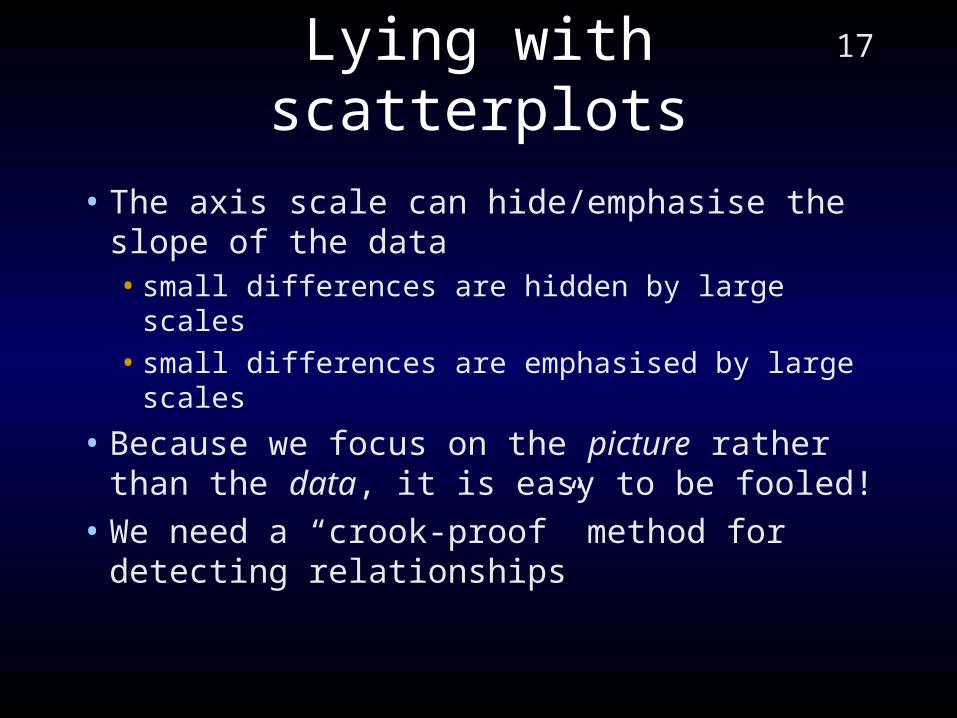
17Lying with scatterplots

• The axis scale can hide/emphasise the slope of the data• small differences are hidden by large scales

• small differences are emphasised by large scales

• Because we focus on the picture rather than the data, it is easy to be fooled!

• We need a “crook-proof” method for detecting relationships

18Co-variance

• Essence of a relship: 2 variables, each exhibiting variance• variation in both temperature and rainfall

• BUT they tend to vary together (change together)

• As one changes, the other changes also

• This behaviour is known as covariance• two variables variances are “tied” to some

degree

• Expressed as a number (eg. cov = 245)

19

Direction of covariance

• Relationships can be positive or negative• Positive: high x implies high y and vice-versa

• Negative: high x implies low y and vice-versa

• We express this “direction” as the sign of the covariance number• pos relationships have pos number (eg. cov =

200)

• neg ones have neg numbers (eg. cov = -200)

20Strength of relationships

• Relationship between calorie intake and weight• For some people: positive relationship (less

calories means less weight; more calories, more weight)

• But for some, it doesn’t work (less calories, same weighr!!)

• This is a weak relationship• only works some of the time

• The stronger a relationship, the more people it occurs in

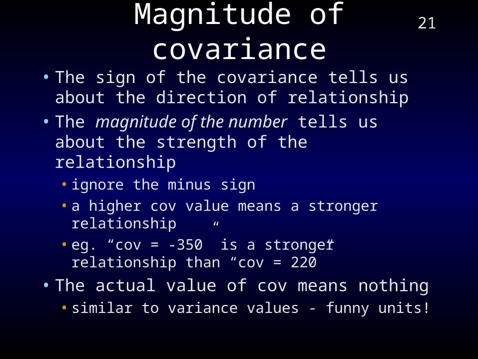
21Magnitude of covariance

• The sign of the covariance tells us about the direction of relationship

• The magnitude of the number tells us about the strength of the relationship• ignore the minus sign

• a higher cov value means a stronger relationship

• eg. “cov = -350” is a stronger relationship than “cov = 220”

• The actual value of cov means nothing• similar to variance values - funny units!

22Pearson’s Product Moment

• A different way to express covariation is to use Pearson’s product moment (“r”)• Uses nice units, can compare across variables

• sometimes incorrectly referred to as “correlation”

• Pearson’s product moment is a standard measure (easy to interpret units)

23Understanding r

• It is written as a single number • eg. r = 0.354

• But is has 2 parts!!• A sign (+ or -)

• A magnitude (the number if you ignore the sign)

• The sign of r is simply the direction of the relationship• a plus: positive relationsip

• a minus: negative relationship

24Understanding r• The magnitude of the sign gives a rough

idea of the strength of the relationship• remember: ignore the sign! (look only at the

number)

• 0 means no relationship at all

• 1 means a perfect, super strong relationship

• Values in between mean varying strength• eg. 0.3 is a weaker relationship than -0.8 (ignore the

sign!!)

• Remember: “strength of relationship” simply means “how many people will it happen for”

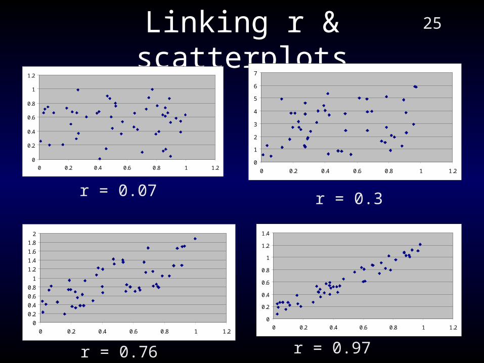
25Linking r & scatterplots

0

0.2

0.4

0.6

0.8

1

1.2

0 0.2 0.4 0.6 0.8 1 1.2

r = 0.07

0

0.2

0.4

0.6

0.8

1

1.2

1.4

1.6

1.8

2

0 0.2 0.4 0.6 0.8 1 1.2

r = 0.76

0

0.2

0.4

0.6

0.8

1

1.2

1.4

0 0.2 0.4 0.6 0.8 1 1.2

r = 0.97

0

1

2

3

4

5

6

7

0 0.2 0.4 0.6 0.8 1 1.2

r = 0.3

26Scatterplots & r

• A low r means the dots are widely scattered

• High r means the dots cluster close by, forming a line

• The direction (sign of r) is simply the slope of the line (up or down)

0

0.2

0.4

0.6

0.8

1

1.2

1.4

0 0.2 0.4 0.6 0.8 1 1.2

r = 0.97

-1.4

-1.2

-1

-0.8

-0.6

-0.4

-0.2

0

0 0.2 0.4 0.6 0.8 1 1.2

r = -0.97

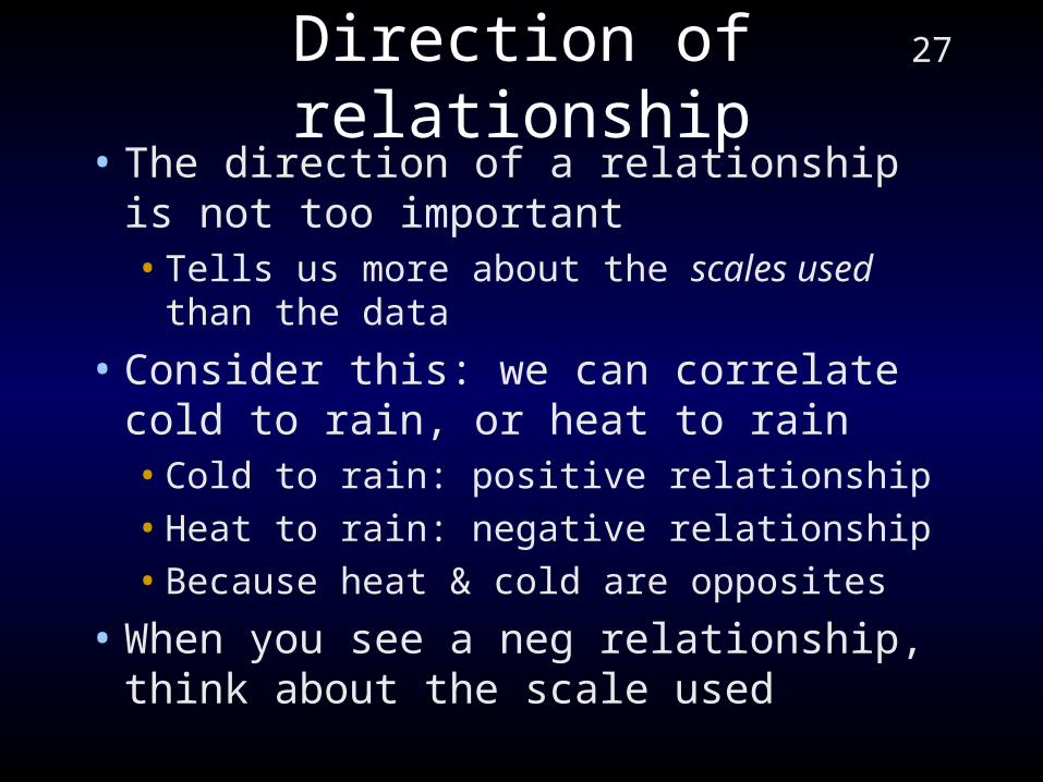
27Direction of relationship

• The direction of a relationship is not too important• Tells us more about the scales used than the

data

• Consider this: we can correlate cold to rain, or heat to rain• Cold to rain: positive relationship

• Heat to rain: negative relationship

• Because heat & cold are opposites

• When you see a neg relationship, think about the scale used

28Statistical Significance of r

• r simply tells you about the sample• need to test its significance to tell if it applies to

the population

• We test the Ho that r=0 (no relationship in the population)

• Use the usual hypothesis testing strategy

29

Statistical significance of r

• If Ho is false, then the relationship we found also applies in the population

• Computer will give you a p value, so it is simple to test• if p is less than your alpha, reject Ho - the

relationship exists in the population

30Strength of r: accurately

• r allows us to look at relationships differently• How closely tied are x and y actually?

• What proportion of the variance of y is actually because of x?• To what extent are the scores of y being

contributed to by x?

31

Example

• Think of somebody’s salary (R4000)• a part of that is due to their education

• a part of it is due to the specific employer

• a part of it is due to the person’s personality

• We can ask: what proportion of that person’s salary is due to their education?• 10%? 50%? 90%?

32

Covariance again

• It is the same with two co-varying variables• Some of the variable’s variance will be due to

the other var

• Some will be due to other factors

• r allows us to accurately pin down this proportion

33Working out the proportion: R2

• To find this proportion simply square your r value• just r2, multiply by 100

• It is actually written with a capital: R2

• Eg. if r = 0.6, then R2 is• 0.6 x 0.6 = 0.36

• 0.36 x 100 = 36

• 36% of the variance of y is due to x