1. Connecting to Matrix Computations - Cornell …math.cornell.edu/~scan/Tensor1.pdf · Four Talks on Tensor Computations 1. Connecting to Matrix Computations Charles F. Van Loan

Four Talks on Tensor Computations

1. Connecting to Matrix Computations

Charles F. Van Loan

Cornell University

SCAN Seminar

October 27, 2014

⊗ Four Talks on Tensor Computations ⊗ 1. Connecting to Matrix Computations 1 / 56

Its About This


Overview

Preparation for the Next Big Thing...

Scalar-Level Thinking

1960’s ⇓

Matrix-Level Thinking

1980’s ⇓

Block Matrix-Level Thinking

2000’s ⇓

Tensor-Level Thinking

⇐ The factorization paradigm:LU, LDLT , QR, UΣV T , etc.

⇐ Cache utilization, parallelcomputing, LAPACK, etc.

⇐New applications, factoriza-tions, data structures, non-linear analysis, optimizationstrategies, etc.


The Matrix Factorizations Paradigm

A = UΣV T PA = LU A = QR A = GGT PAPT = LDLT QTAQ = DX−1AX = J UTAU = T AP = QR A = ULV T PAQT = LU A = UΣV T

PA = LU A = QR A = GGT PAPT = LDLT QTAQ = D X−1AX = JUTAU = T AP = QR A = ULV T PAQT = LU A = UΣV T PA = LUA = QR A = GGT PAPT = LDLT QTAQ = D X−1AX = J UTAU = TAP = QR A = ULV T PAQT = LU A = UΣV T PA = LU A = QRA = GGT PAPT = LDLT QTAQ = D X−1AX = J UTAU = TA = ULV T PAQT = LU A = UΣV T PA = LU A = QR A = GGT

PAPT = LDLT QTAQ = D X−1AX = J UTAU = T AP = QRA = ULV T PAQT = LU A = UΣV T PA = LU A = QR A = GGT

PAPT = LDLT QTAQ = D X−1AX = J AP = QR A = ULV T

PAQT = LU A = UΣV T PA = LU A = QR A = GGT PAPT = LDLT

QTAQ = D X−1AX = J UTAU = T AP = QR A = ULV T PAQT = LUA = UΣV T PA = LU A = QR A = GGT PAPT = LDLT QTAQ = DX−1AX = J UTAU = T AP = QR A = ULV T PAQT = LU A = UΣV T

PA = LU A = QR PAPT = LDLT QTAQ = D X−1AX = J UTAU = TAP = QR A = ULV T PAQT = LU A = UΣV T PA = LU A = QR

It’s a Language


Some Ways They Are Used

Conversion of a “hard” matrix problem into an easier one.

Ax = b ≡ Ly = Pb, Ux = y

Low-rank approximation.

(107-by-105) ≈ (107-by-10)× (10-by-105)

Reasoning about Data Re-Use via Block Factorizations

Aij ← Aij − AikAkj not aij ← aij − aikakj

Discovery and Insight

minQ,x ,y

‖ A1 − (A2 + xyT )Q ‖F ≤ 10−4


Tensor Factorizations and Decompositions

The same story is playing out with tensors:

= σ1 w1 ◦ v1 ◦ u1 + σ2 w2 ◦ v2 ◦ u2 + . . .


The Big Data Theme

A Changing Definition of “Big”

In Matrix Computations, to say that A ∈ IRn1×n2 is “big” is to saythat both n1 and n2 are big.

In Tensor Computations, to say that A ∈ IRn1×···×nd is “big” is to saythat n1n2 · · · nd is big and this need not require big nk . E.g.n1 = n2 = · · · = n1000 = 2.

Algorithms that scale with d will induce a transition...

Matrix-Based Scientific Computation

⇓Tensor-Based Scientific Computation


What is a Tensor?

Definition

An order-d tensor A ∈ IRn1×···×nd is a real d-dimensional arrayA(1:n1, . . . , 1:nd) where the index range in the k-th mode is from 1to nk . A tensor A ∈ IRn1×···×nd is cubical if n1 = · · · = nd .

Low-Order Tensors

A scalar is an order-0 tensor.

A vector is an order-1 tensor.

A matrix is an order-2 tensor.

We use calligraphic font to designate tensors that have order 3 or greatere.g., A, B, C, etc.


Where Might They Come From?

Discretization

A(i , j , k, `) might house the value of f (w , x , y , z) at(w , x , y , z) = (wi , xj , yk , z`).

Multiway Analysis

A(i , j , k, `) is a value that captures an interaction between fourvariables/factors.


You Have Seen Them Before

Images

A color picture is an m-by-n-by-3 tensor:

A(:, :, 1) = red pixel values

A(:, :, 2) = green pixel values

A(:, :, 3) = blue pixel values

Obvious extension of the “colon notation”. More later.


You Have Seen them Before

Block Matrices

A =

a11 a12 a13 a14 a15 a16

a21 a22 a23 a24 a25 a26

a31 a32 a33 a34 a35 a36

a41 a42 a43 a44 a45 a46

a51 a52 a53 a54 a55 a56

a61 a62 a63 a64 a65 a66

Matrix entry a45 is the (2,1) entry of the (2,3) block:

a45 ⇔ A(2, 3, 2, 1)


You Have Seen them Before

Kronecker Products

The m1m2m3-by-n1n2n3 matrix

A = A1(1:m1, 1:n1)⊗ A2(1:m2, 1:n2)⊗ A3(1:m3, 1:n3)

is a reshaping of the m1-by-m2-by-m3-by-n1-by-n2-by-n3 tensor

A(i1, i2, i3, j1, j2, j3) = A1(i1, j1)A2(i2, j2)A3(i3, j3)


The Kronecker Product

Definition

B ⊗ C is a block matrix whose ij-th block is bijC .

An Example... [b11 b12

b21 b22

]⊗ C =

[b11C b12C

b21C b22C

]

Kronecker products have a replicated block structure.



There are three ways to regard A = B ⊗ C ...

If

A =

b11 · · · b1n...

. . ....

bm1 · · · bmn

⊗ c11 · · · c1q

.... . .

...cp1 · · · cpq

then

(i). A is an m-by-n block matrix with p-by-q blocks.

(ii). A is an mp-by-nq matrix of scalars.

(iii). A is an unfolded 4-th order tensor A ∈ IRp×q×m×n:

A(i1, i2, i3, i4) = B(i3, i4)C (i1, i2)


Kronecker Product: All Possible Entry-Entry Products

4× 9 = 36

[b11 b12

b21 b22

]⊗

c11 c12 c13

c21 c22 c23

c31 c32 c33

=

b11c11 b11c12 b11c13 b12c11 b12c12 b12c13

b11c21 b11c22 b11c23 b12c21 b12c22 b12c23

b11c31 b11c32 b11c33 b12c31 b12c32 b12c33

b21c11 b21c12 b21c13 b22c11 b22c12 b22c13

b21c21 b21c22 b21c23 b22c21 b22c22 b22c23

b21c31 b21c32 b21c33 b22c31 b22c32 b22c33


Kronecker Products of Kronecker Products

Hierarchical

B ⊗ C ⊗ D=[

b11 b12

b21 b22

]⊗

c11 c12 c13 c14

c21 c22 c23 c24

c31 c32 c33 c34

c41 c42 c43 c44

⊗ d11 d12 d13

d21 d22 d23

d31 d32 d33

A 2-by-2 block matrix whose entries are 4-by-4 block matrices whose entriesare 3-by-3 matrices.


Bridging the Gap to Matrix Computations

Tensor computations are typically disguised matrix computations andthat is because of


A = A1 ⊗ A2 ⊗ A3 an order 6 tensor

Tensor Unfoldings

Rubik Cube −→ 3× 9 matrix

Alternating Least Squares

Multilinear optimization via component-wise optimization


The Decomposition Paradigm in Matrix Computations

Typical...

Convert the given problem into an equivalent easy-to-solve problemby using the “right” matrix decomposition.

PA = LU, Ly = Pb, Ux = y =⇒ Ax = b

Also Typical...

Uncover hidden relationships by computing the “right” decompositionof the data matrix.

A = UΣV T =⇒ A ≈r∑

i=1

σiuivTi


Two Natural Questions

Question 1

Can we solve tensor problems by converting them to equivalent,easy-to-solve problems using a tensor decomposition?

Question 2

Can we uncover hidden patterns in tensor data by computing anappropriate tensor decomposition?

Let’s explore the decomposition issue for 2-by-2-by-2 tensors...


The Singular Value Decomposition

The 2-by-2 case...

[a11 a12

a21 a22

]=

[u11 u12

u21 u22

] [σ1 00 σ2

] [v11 v12

v21 v22

]T

= σ1

[u11

u21

] [v11

v21

]T

+ σ2

[u12

u22

] [v12

v22

]T

A reshaped presentation of the same thing...a11

a21

a12

a22

= σ1

v11u11

v11u21

v21u11

v21u21

+ σ2

v12u12

v12u22

v22u12

v22u22

The reshaped rank-1 matrices have special structure...


The Kronecker Product (KP)

The KP of a Pair of 2-vectors

[x1

x2

]⊗

[y1

y2

]=

x1y1

x1y2

x2y1

x2y2

2-by-2 SVD in KP Terms...

a11

a21

a12

a22

= σ1

[v11

v21

]⊗

[u11

u21

]+ σ2

[v12

v22

]⊗

[u12

u22

]


Reshaping

Appreciate the Duality..

[a11 a12

a21 a22

]= σ1 · u1v

T1 + σ2 · u2v

T2

a11

a21

a12

a22

= σ1 · (v1 ⊗ u1) + σ2 · (v2 ⊗ u1)

U =[

u1 u2

]V =

[v1 v2

]


A ∈ IR2×2×2 as a minimal sum of rank-1 tensors.

What is a rank-1 tensor?

If R ∈ IR2×2×2 has unit rank, then there exist f , g , h ∈ IR2 such that

r111

r211

r121

r221

r112

r212

r122

r222

=

[h1

h2

]⊗

[g1

g2

]⊗

[f1f2

]

This means that if R = (rijk), then

rijk = hk · gj · fi i = 1:2, j = 1:2, k = 1:2



Challenge: Find thinnest possible X ,Y ,Z ∈ IR2×r so

a111

a211

a121

a221

a112

a212

a122

a222

=

r∑k=1

zk ⊗ yk ⊗ xk

where X = [ x1| · · · |xr ], Y = [ y1| · · · |yr ], andZ = [ z1| · · · |zr ] arecolumn partitionings.

The minimizing r is the tensor rank.



A Surprising Fact

If

a111

a211

a121

a221

a112

a212

a122

a222

= randn(8,1), then

rank = 2 with prob 79%

rank = 3 with prob 21%

This is Different from the Matrix Case...

If A = randn(n,n), then rank(A) = n with prob 100%.

What are the “full rank” 2-by-2-by-2 tensors?


The 79/21 Property

The 2-by-2 Generalized Eigenvalue Problem (GEV)

The generalized eigenvalues of F − λG are the zeros of

det

([f11 f12

f21 f22

]− λ

[g11 g12

g21 g22

])= 0

Coincidence?

If the aijk are randn, then

det

([a111 a121

a211 a221

]− λ

[a112 a122

a212 a222

])= 0

has real distinct roots with probability 79% and complex conjugateroots with probability 21%.

What is the connection between the 2-by-2 GEV and the 2-by-2-by-2 tensorrank problem?


Nearness Problems

The Nearest Rank-1 Matrix Problem

If A ∈ IRn1×n2 has SVD A = UΣV T then Bopt = σ1u1vT1 minimizes

φ(B) = ‖ A− B ‖F rank(B) = 1.

The Nearest Rank-1 Tensor Problem for A ∈ IR2×2×2

Find unit 2-norm vectors u, v ,w ∈ IR2 and scalar σ so that‖ a− σ · w ⊗ v ⊗ u ‖2 is minimized where

a =

a111

a211

a121

a221

a112

a212

a122

a222


A Highly Structured Nonlinear Optimization Problem

It Depends on Four Parameters...

φ(σ, θ1, θ2, θ3) =

∥∥∥∥a − σ

[cos(θ3)sin(θ3)

]⊗

[cos(θ2)sin(θ2)

]⊗

[cos(θ1)sin(θ1)

]∥∥∥∥2

=

∥∥∥∥∥∥∥∥∥∥∥∥∥∥∥∥

a111

a211

a121

a221

a112

a212

a122

a222

− σ ·

c3c2c1

c3c2s1c3s2c1

c3s2s1s3c2c1

s3c2s1s3s2c1

s3s2s1

∥∥∥∥∥∥∥∥∥∥∥∥∥∥∥∥2

ci = cos(θi ), si = sin(θi ) i = 1:3



And It Can Be Reshaped...

φ =

‚‚‚‚‚‚‚‚‚‚‚‚‚‚‚‚

266666666664

a111

a211

a121

a221

a112

a212

a122

a222

377777777775− σ ·

266666666664

c3c2c1

c3c2s1

c3s2c1

c3s2s1

s3c2c1

s3c2s1

s3s2c1

s3s2s1

377777777775

‚‚‚‚‚‚‚‚‚‚‚‚‚‚‚‚2

=

‚‚‚‚‚‚‚‚‚‚‚‚‚‚‚‚

266666666664

a111

a211

a121

a221

a112

a212

a122

a222

377777777775−

266666666664

c3c2 00 c3c2

c3s2 00 c3s2

s3c2 00 s3c2

s3s2 00 s3s2

377777777775

»x1

y1

– ‚‚‚‚‚‚‚‚‚‚‚‚‚‚‚‚2

[x1

y1

]= σ ·

[c1

s1

]= σ ·

[cos(θ1)sin(θ1)

]Idea: Improve σ and θ1 by minimizing with respect to x1 and y1, holding θ2

and θ3 fixed.




φ =

‚‚‚‚‚‚‚‚‚‚‚‚‚‚‚‚

266666666664

a111

a211

a121

a221

a112

a212

a122

a222

377777777775− σ ·

266666666664

c3c2c1

c3c2s1

c3s2c1

c3s2s1

s3c2c1

s3c2s1

s3s2c1

s3s2s1

377777777775

‚‚‚‚‚‚‚‚‚‚‚‚‚‚‚‚2

=

‚‚‚‚‚‚‚‚‚‚‚‚‚‚‚‚

266666666664

a111

a211

a121

a221

a112

a212

a122

a222

377777777775−

266666666664

c3c1 0c3s1 00 c3c1

0 c3s1

s3c1 0s3s1 00 s3c1

0 s3s1

377777777775

»x2

y2

– ‚‚‚‚‚‚‚‚‚‚‚‚‚‚‚‚2

[x2

y2

]= σ ·

[c2

s2

]= σ ·

[cos(θ2)sin(θ2)


and θ3 fixed.




φ =

‚‚‚‚‚‚‚‚‚‚‚‚‚‚‚‚

266666666664

a111

a211

a121

a221

a112

a212

a122

a222

377777777775− σ ·

266666666664

c3c2c1

c3c2s1

c3s2c1

c3s2s1

s3c2c1

s3c2s1

s3s2c1

s3s2s1

377777777775

‚‚‚‚‚‚‚‚‚‚‚‚‚‚‚‚2

=

‚‚‚‚‚‚‚‚‚‚‚‚‚‚‚‚

266666666664

a111

a211

a121

a221

a112

a212

a122

a222

377777777775−

266666666664

c2c1 0c2s1 0s2c1 0s2s1 00 c2s1

0 c2s1

0 s2c1

0 s2s1

377777777775

»x3

y3

– ‚‚‚‚‚‚‚‚‚‚‚‚‚‚‚‚2

[x3

y3

]= σ ·

[c3

s3

]= σ ·

[cos(θ3)sin(θ3)


and θ2 fixed.


Componentwise Optimization

A Common Framework for Tensor-Related Optimization

Choose a subset of the unknowns such that if they are(temporarily) fixed, then we are presented with some standardmatrix problem in the remaining unknowns.

By choosing different subsets, cycle through all the unknowns.

Repeat until converged.

In tensor computations, the “standard matrix problem” that we end upsolving is usually the linear least squares problem. In that case, the overall

solution process is referred to as alternating least squares.


Bridging the Gap via Tensor Unfoldings

A Common Framework for Tensor Computations...

1. Turn tensor A into a matrix A.

2. Through matrix computations, discover things about A.

3. Draw conclusions about tensor A based on what is learned aboutmatrix A.


Tensor Unfoldings

Some Tensor Unfoldings of A ∈ IR4×3×2

A(1) =

2664a111 a121 a131 a112 a122 a132

a211 a221 a231 a212 a222 a232

a311 a321 a331 a312 a322 a332

a411 a421 a431 a412 a422 a432

3775

A(2) =

24 a111 a211 a311 a411 a112 a212 a312 a412

a121 a221 a321 a421 a122 a222 a322 a422

a131 a231 a331 a431 a132 a232 a332 a432

35A(3) =

»a111 a211 a311 a411 a121 a221 a321 a421 a131 a231 a331 a431

a112 a212 a312 a412 a122 a222 a322 a422 a132 a232 a332 a432

–

A “tensor unfolding” is sometimes referred to as “tensor flattening” or as a“tensor matricization.”


Tensor Unfoldings: How They Might Show Up

Gradients of Multilinear Forms

If f :IRn1 × IRn2 × IRn3 → IR is defined by

f (u, v ,w) =n1∑

i1=1

n2∑i2=1

n3∑i3=1

A(i1, i2, i3)u(i1)v(i2)w(i3)

and A ∈ IRn1×n2×n3 , then its gradient is given by

∇f (u, v ,w) =

A(1) w ⊗ v

A(2) w ⊗ u

A(3) v ⊗ u

where A(1), A(2), and A(3) are the modal unfoldings of A.


More General Unfoldings

Example: A = A(1:2, 1:3, 1:2, 1:2, 1:3)

B =

(1,1) (2,1) (1,2) (2,2) (1,3) (2,3)2666666666666666666666664

a11111 a11121 a11112 a11122 a11113 a11123

a21111 a21121 a21112 a21122 a21113 a21123

a12111 a12121 a12112 a12122 a12113 a12123

a22111 a22121 a22112 a22122 a22113 a22123

a13111 a13121 a13112 a13122 a13113 a13123

a23111 a23121 a23112 a23122 a23113 a23123

a11211 a11221 a11212 a11222 a11213 a11223

a21211 a21221 a21212 a21222 a21213 a21223

a12211 a12221 a12212 a12222 a12213 a12223

a22211 a22221 a22212 a22222 a22213 a22223

a13211 a13221 a13212 a13222 a13213 a13223

a23211 a23221 a23212 a23222 a23213 a23223

3777777777777777777777775

(1,1,1)

(2,1,1)

(1,2,1)

(2,2,1)

(1,3,1)

(2,3,1)

(1,1,2)

(2,1,2)

(1,2,2)

(2,2,2)

(1,3,2)

(2,3,2)


A Block Matrix is an Unfolded Order-4 Tensor

Some Natural Identifications

A block matrix with uniformly sized blocks

A =

A11 · · · A1,c2

.... . .

...Ar2,1 · · · Ar2,c2

Ai2,j2 ∈ IRr1×c1

has several natural reshapings:

Ai1,j1(i2, j2) ↔ A(i1, j1, i2, j2) A ∈ IRr1×r2×c1×c2

Ai2,j2(i1, j1) ↔ A(i1, j1, i2, j2) A ∈ IRr1×c1×r2×c2


Kronecker Products are Unfolded Tensors

The m1m2m3-by-n1n2n3 matrix

A = A1(1:m1, 1:n1)⊗ A2(1:m2, 1:n2)⊗ A3(1:m3, 1:n3)

is a particular unfolding of the m1-by-m2-by-m3-by-n1-by-n2-by-n3

tensor

A(i1, i2, i3, j1, j2, j3) = A1(i1, j1)A2(i2, j2)A3(i3, j3)


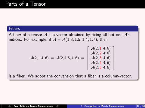
Parts of a Tensor

Fibers

A fiber of a tensor A is a vector obtained by fixing all but one A’sindices. For example, if A = A(1:3, 1:5, 1:4, 1:7), then

A(2, :, 4, 6) = A(2, 1:5, 4, 6) =

A(2, 1, 4, 6)A(2, 2, 4, 6)A(2, 3, 4, 6)A(2, 4, 4, 6)A(2, 5, 4, 6)

is a fiber. We adopt the convention that a fiber is a column-vector.


The vec Operation

Turns matrices into vectors by stacking columns...

X =

1 102 203 30

⇒ vec(X ) =

123102030


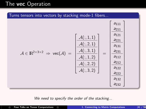
The vec Operation

Turns tensors into vectors by stacking mode-1 fibers...

A ∈ IR2×3×2 ⇒ vec(A) =

A(:, 1, 1)

A(:, 2, 1)

A(:, 3, 1)

A(:, 1, 2)

A(:, 2, 2)

A(:, 3, 2)

=

a111

a211

a121

a221

a131

a231

a112

a212

a122

a222

a132

a232

We need to specify the order of the stacking...


Parts of a Tensor

Slices

A slice of a tensor A is a matrix obtained by fixing all but two of A’sindices. For example, if A = A(1:3, 1:5, 1:4, 1:7), then

A(:, 3, :, 6) =

A(1, 3, 1, 6) A(1, 3, 2, 6) A(1, 3, 3, 6) A(1, 3, 4, 6)A(2, 3, 1, 6) A(2, 3, 2, 6) A(2, 3, 3, 6) A(2, 3, 4, 6)A(3, 3, 1, 6) A(3, 3, 2, 6) A(3, 3, 3, 6) A(3, 3, 4, 6)

is a slice. We adopt the convention that the first unfixed index in thetensor is the row index of the slice and the second unfixed index inthe tensor is the column index of the slice.


Tensor Notation: Subscript Vectors

Referencing a Tensor Entry

If A ∈ IRn1×···×nd and i = (i1, . . . , id) with 1 ≤ ik ≤ nk for k = 1:d ,then

A(i) ≡ A(i1, . . . , ik)

We say that i is a subscript vector. Bold font will be used designatesubscript vectors.

Bounding Subscript Vectors

If L and R are subscript vectors having the same dimension, thenL ≤ R means that Lk ≤ Rk for all k.

Special Subscript Vectors

The subscript vector of all ones is denoted by 1. (Dimension clearfrom context.) If N is an integer, then N = N · 1.


Subtensors

Specification of Subtensors

Suppose A ∈ IRn1×···×nd with n = [ n1, . . . , nd ]. If 1 ≤ L ≤ R ≤ n,then A(L:R) denotes the subtensor

B = A(L1:R1, . . . , Ld :Rd)


The Index-Mapping Function col

Definition

If i and n are length-d subscript vectors, then the integer-valuedfunction col(i,n) is defined by

col(i,n) = i1 + (i2 − 1)n1 + (i3 − 1)n1n2 + · · ·+ (id − 1)n1 · · · nd−1

The Formal Specification of Vec

If A ∈ IRn1×···×nd and v = vec(A), then

a (col(i,n)) = A(i) 1 ≤ i ≤ n


The Importance of Notation

Contractions

A(i1, i2, j1, j2, j3) =∑k1

∑k2

B(i1, i2, k1, k2)C(k1, k2, j1, j2, j3)

is better written as

A(i, j) =∑k

B(i, k)C(k, j)


Software: The Matlab Tensor Toolbox

Why?

It provides an excellent environment for learning about tensorcomputations and for building a facility with multi-index reasoning.

Who?

Brett W. Bader and Tamara G. Kolda, Sandia Laboratories

Where?

http://csmr.ca.sandia.gov/∼tkolda/TensorToolbox/


Matlab Tensor Toolbox: A Tensor is a Structure

>> n = [3 5 4 7];

>> A_array = randn(n);

>> A = tensor(A_array );

>> fieldnames(A)

ans =

’data’

’size’

The .data field is a multi-dimensional array.

The .size field is an integer vector that specifies the modal dimensions.

A.data and A array have same value.

A.size and n have the same value.


Matlab Tensor Toolbox: Order and Dimension

>> n = [3 5 4 7];

>> A_array = randn(n);

>> A = tensor(A_array)

>> d = ndims(A)

d =

4

>> n = size(A)

n =

3 5 4 7


Matlab Tensor Toolbox: Tensor Operations

n = [3 5 4 7];

% Familiar initializations ...

X = tenzeros(n); Y = tenones(n);

A = tenrand(n); B = tenrand(n);

% Extracting Fibers and Slices

a_Fiber = A(2,:,3,6); a_Slice = A(3,:,2,:);

% These operations are legal ...

C = 3*A; C = -A; C = A+1; C = A.^2;

C = A + B; C = A./B; C = A.*B; C = A.^B;

% Frobenius norm ...

err = norm(A);

% Applying a Function to Each Entry ...

F = tenfun(@sin ,A);

G = tenfun(@(x) sin(x)./exp(x),A);


The Matlab Tensor Toolbox

Problem 1. Suppose A = A(1:n1, 1:n2, 1:n3). We say A(i) is an interiorentry if 1 < i < n. Otherwise, we say A(i) is an edge entry. If A(i1, i2, i3) isan interior entry, then it has six neighbors: A(i1 ± 1, i2, i3),A(i1, i2 ± 1, i3),and A(i1, i2, i3 ± 1). Implement the following function so that it performsas specified

function B = Smooth(A)

% A is a third order tensor

% B is a third order tensor with the property that each

% interior entry B(i) is the average of A(i)’s six

% neighbors. If B(i) is an edge entry, then B(i) = A(i).

Strive for an implementation that does not have any loops.

Problem 2. Formulate and solve an order-d version of Problem 1.


Modal Unfoldings Using tenmat

Example: A Mode-2 Unfolding of A ∈ IR4×3×2

tenmat(A,2) sets up A(2): a111 a211 a311 a411 a112 a212 a312 a412

a121 a221 a321 a421 a122 a222 a322 a422

a131 a231 a331 a431 a132 a232 a332 a432

(1,1) (2,1) (3,1) (4,1) (1,2) (2,2) (3,2) (4,2)

Notice how the fibers are ordered.


Modal Unfoldings Using tenmat

Precisely how are the fibers ordered?

If A ∈ IRn1×···×nd , N = n1 · · · nd , and B = tenmat(A,k), then B isthe matrix A(k) ∈ IRnk×(N/nk ) with

A(k)(ik , col(ik, n)) = A(i)where

ik = [i1, . . . , ik−1, ik+1, . . . , id ]

nk = [n1, . . . , nk−1, nk+1, . . . ,md ]

Recall that the col function maps multi-indices to integers. For example, ifn = [2 3 2] then

i (1, 1, 1) (2, 1, 1) 1, 2, 1) (2, 2, 1) (1, 3, 1) (2, 3, 1) (1, 1, 2) (2, 1, 2) ...col(i, n) 1 2 3 4 5 6 7 8 ...


Matlab Tensor Toolbox: A Tenmat Is a Structure

>> n = [3 5 4 7];

>> A = tenrand(n);

>> A2 = tenmat(A,2);

>> fieldnames(A2)

ans =

’tsize ’

’rindices ’

’cindices ’

’data’

A2.tsize = size of the unfolded tensor = [3 5 4 7]A2.rindices = mode indices that define A2’s rows = [2]A2.cindices = mode indices that define A2’s columns = [1 3 4]A2.data = the matrix that is the unfolded tensor.


Other Modal Unfoldings Using tenmat

Mode-k Unfoldings of A ∈ IRn1×···×nd

A particular mode-k unfolding is defined by a permutation v of[1:k − 1 k + 1:d

]. Tensor entries get mapped to matrix entries as

followsA(i) → A(ik , col(i(v),n(v)))

Name v How to get it...

A(k) (Default) [1:k−1 k+1:d ] tenmat(A,k)

Forward Cyclic [k + 1:d 1:k−1] tenmat(A,k,’fc’)

Backward Cyclic [k − 1:− 1:1 d :−1:k+1] tenmat(A,k,’bc’)

Arbitrary v tenmat(A,k,v)


Using tenmat

Problem 3. Write a Matlab function alpha = MaxFnorm(A) that returnsthe maximum value of ‖ B ‖F where B is a slice of the input tensorA ∈ IRn1×···×nd .


Summary

Key Words

Reshaping is about turning a matrix in to a differently sizedmatrix or into a tensor or into a vector.

The Kronecker product is an operation between two matricesthat produces a highly structured block matrix.

A Rank-1 tensor can be reshaped into a multiple Kroneckerproduct of vectors.

A tensor decomposition expresses a given tensor in terms ofsimpler tensors.

The alternating least squares approach to multilinear LS is basedon solving a sequence of linear LS problems, each obtained byfreezing all but a subset of the unknowns.


Summary

Key Words

A block matrix is a matrix whose entries are matrices.

A fiber of a tensor is a column vector defined by fixing all butone index and varying what’s left. A slice of a tensor is a matrixdefined by fixing all but two indices and varying what’s left.

A mode-k unfolding of a tensor is obtained by assembling all themode-k fibers into a matrix.

tensor is a Tensor Toolbox command used to construct tensors.

tenmat is a Tensor Toolbox command that is used to constructunfoldings of a tensor.


Summary

Recurring themes...

Given tensor A ∈ IRn1×···×nd , there are many ways to unfold a tensorinto a matrix A ∈ IRN1×N2 where N1N2 = n1 · · · nd .

For example, A could be a block matrix whose entries are A-slices.

A facility with block matrices and tensor indexing is required tounderstand the layout possibilities.

Computations with the unfolded tensor frequently involve theKronecker product.


References

L. De Lathauwer and B. De Moor (1998). “From Matrix to Tensor: MultilinearAlgebra and Signal Processing,” in Mathematics in Signal Processing IV, J.McWhirter and I. Proudler, eds., Clarendon Press, Oxford, 1–15.

G.H. Golub and C. Van Loan (2013). Matrix Computations, 4th Edition, JohnsHopkins University Press, Baltimore, MD.

T.G. Kolda and B.W. Bader (2009). “Tensor Decompositions and Applications,”SIAM Review 51, 455–500.

P.M. Kroonenberg (2008). Applied Multiway Data Analysis, Wiley.

A. Smilde, R. Bro, and P. Geladi (2004). Multi-Way Analysis: Applications in theChemical Sciences, Wiley, West Sussex, England.

B.W. Bader and T.G. Kolda (2006). “Algorithm 862: MATLAB Tensor Classes forFast Algorithm Prototyping,” ACM Transactions on Mathematical Software,32, 635–653.


Documents

1. Connecting to Matrix Computations - Cornell …math.cornell.edu/~scan/Tensor1.pdf · Four Talks on Tensor Computations 1. Connecting to Matrix Computations Charles F. Van Loan