1

ConfoundingConfounding

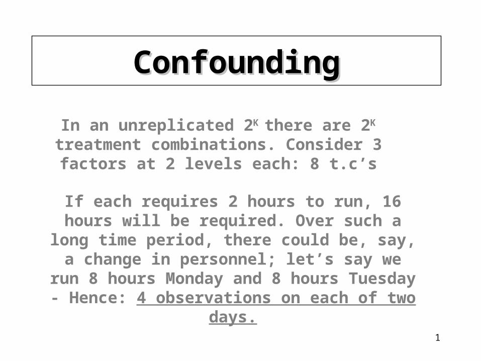
In an unreplicated 2K there are 2K treatment combinations. Consider 3 factors at 2 levels

each: 8 t.c’s

If each requires 2 hours to run, 16 hours will be required. Over such a long time period, there

could be, say, a change in personnel; let’s say we run 8 hours Monday and 8 hours Tuesday -

Hence: 4 observations on each of two days.

2

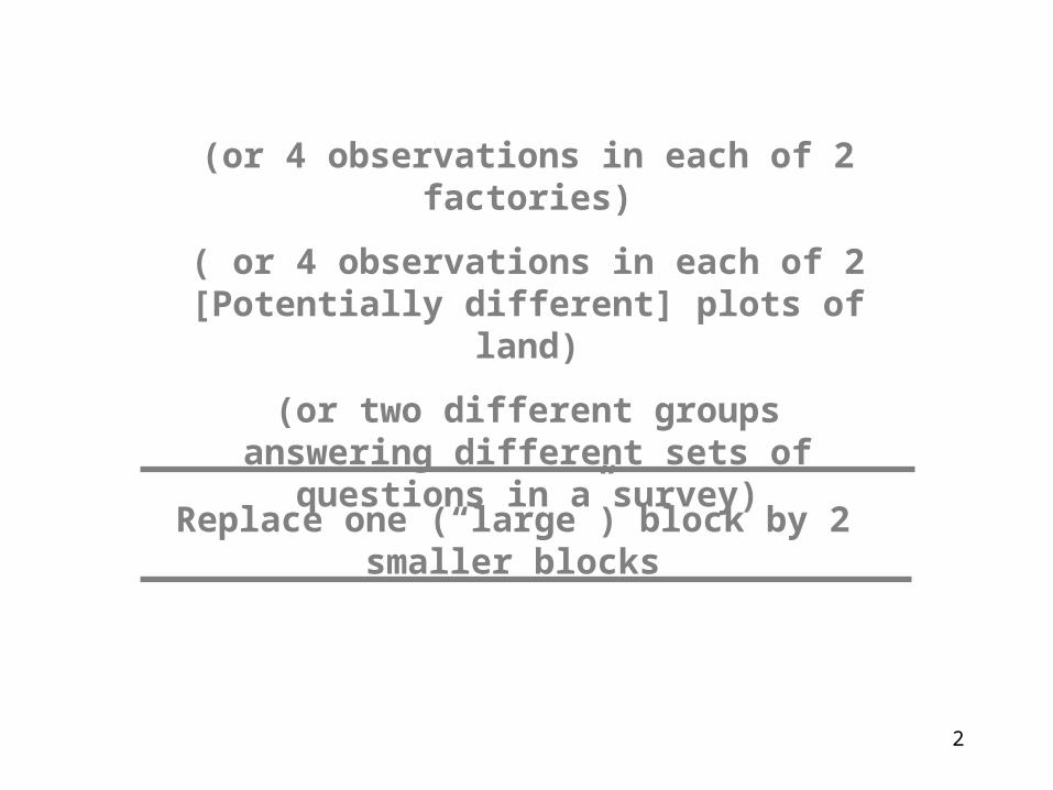
(or 4 observations in each of 2 factories)

( or 4 observations in each of 2 [Potentially different] plots of land)

(or two different groups answering different sets of questions in a survey)

Replace one (“large”) block by 2 smaller blocks

3

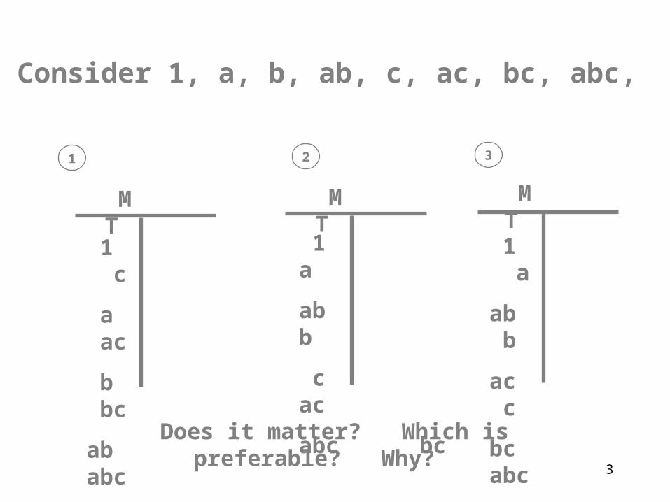
Consider 1, a, b, ab, c, ac, bc, abc,

M T

1

1 a

ab b

c ac

abc bc

M T

1 c

a ac

b bc

ab abc

M T

1 a

ab b

ac c

bc abc

32

Does it matter? Which is preferable? Why?

4

The block with the “1” observation (everything at low level) is called the “Principal block”. (It

has equal stature with other blocks, but is useful to identify.)

Assume all Monday yields are higher than Tuesday yields by a (near) constant but unknown amount X. (X is in units of the

dependent variable under study).

What is the consequence(s) of having 2 smaller blocks?

5

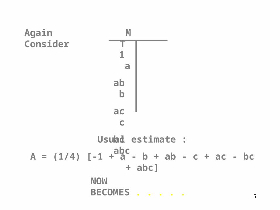
Again Consider

M T

1 a

ab b

ac c

bc abc

Usual estimate :

A = (1/4) [-1 + a - b + ab - c + ac - bc + abc]

NOW BECOMES . . . . .

6

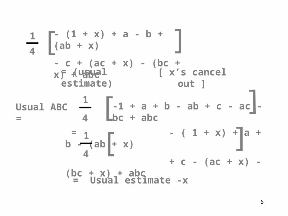
Usual ABC = 1

4 [ -1 + a + b - ab + c - ac - bc + abc [

= - ( 1 + x) + a + b - (ab + x)

+ c - (ac + x) - (bc + x) + abc

1

4 [

[

= Usual estimate -x

1

4

- (1 + x) + a - b + (ab + x)

- c + (ac + x) - (bc + x) + abc [

[

= (usual estimate) [ x’s cancel out ]

7

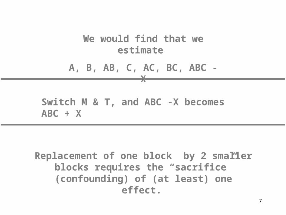
We would find that we estimate

A, B, AB, C, AC, BC, ABC - X

Switch M & T, and ABC -X becomes ABC + X

Replacement of one block by 2 smaller blocks requires the “sacrifice” (confounding) of (at

least) one effect.

8

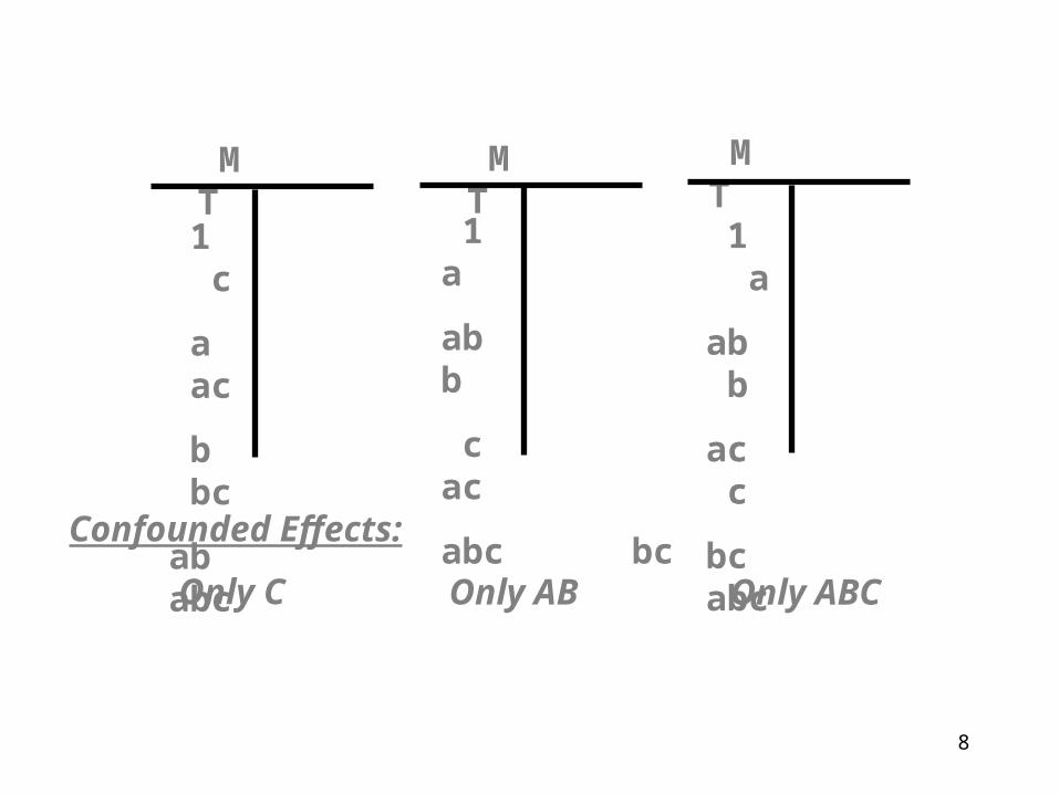
M T

1 a

ab b

c ac

abc bc

M T

1 c

a ac

b bc

ab abc

M T

1 a

ab b

ac c

bc abc

Confounded Effects:

Only C Only AB Only ABC

9

Confounded Effects:

B, C,

AB,

AC

M T

1 ab

a c

b bc

ac abc

(4 out of 7, instead of 1 out of 7)

10

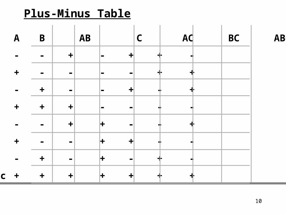
A B AB C AC BC ABC

1 - - + - + + -

a + - - - - + +

b - + - - + - +

ab + + + - - - -

c - - + + - - +

ac + - - + + - -

bc - + - + - + -

abc + + + + + + +

A B AB C AC BC ABC

1 - - + - + + -

a + - - - - + +

b - + - - + - +

ab + + + - - - -

c - - + + - - +

ac + - - + + - -

bc - + - + - + -

abc + + + + + + +

Plus-Minus Table

11

Recall: X is “nearly constant”. If X varies significantly with t.c.’s, it interacts with A/B/C, etc., and should be included as an additional factor.

12

Basic idea can be viewed as follows:

STUDY IMPORTANT FACTORS UNDER MORE HOMOGENEOUS CONDITIONS, With the influence of some of the heterogeneity in yields caused by unstudied factors confined to one effect, (generally the one we’re least interested in estimating - often one we’re willing to assume equals zero - usually the highest order interaction). We reduce Exp. Error by creating 2 smaller blocks, at expense of confounding one effect.

13

All estimates not “lost” can be judged against less variability (and hence, we get narrower

confidence intervals, smaller error for given error, etc.)

For K large in 2k, confounding is popular - Why?

(1) it is difficult to create large homogeneous blocks.

(2) loss of one effect is not thought to be important.

(e.g., in 27, we give up 1 out of 127 effects - perhaps ABCDEFG)

14

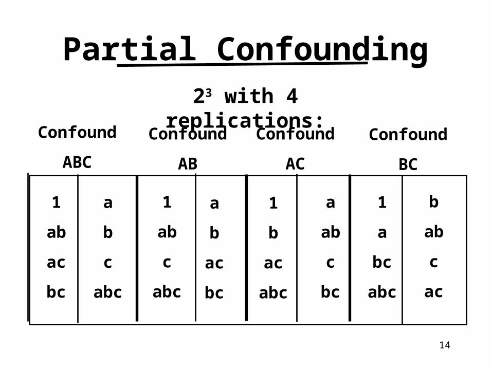
Partial Confounding23 with 4 replications:

Confound

ABC

Confound

AC

Confound

BC

Confound

AB

1

ab

ac

bc

a

b

c

abc

1

ab

c

abc

a

b

ac

bc

1

b

ac

abc

a

ab

c

bc

1

a

bc

abc

b

ab

c

ac

15

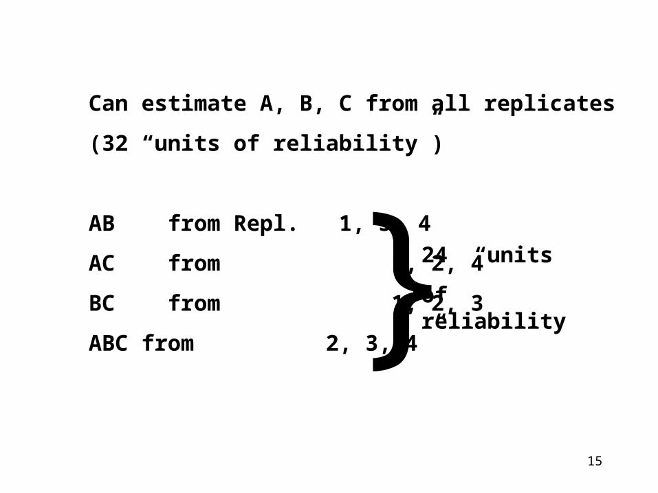
Can estimate A, B, C from all replicates

(32 “units of reliability”)

AB from Repl. 1, 3, 4

AC from 1, 2, 4

BC from 1, 2, 3

ABC from 2, 3, 4 } 24 “units

of reliability”

16

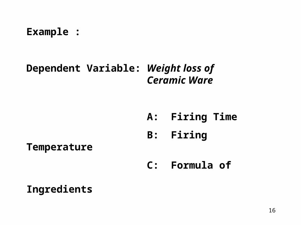
Example :

Dependent Variable: Weight loss of Ceramic Ware

A: Firing Time

B: Firing Temperature

C: Formula of Ingredients

17

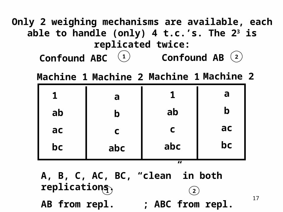
Only 2 weighing mechanisms are available, each able to handle (only) 4 t.c.’s. The 23 is replicated twice:

1

ab

ac

bc

a

b

c

abc

1

ab

c

abc

a

b

ac

bc

Machine 1 Machine 2 Machine 1 Machine 2

Confound ABC 1 Confound AB 2

A, B, C, AC, BC, “clean” in both replications.

AB from repl. ; ABC from repl. 1 2

18

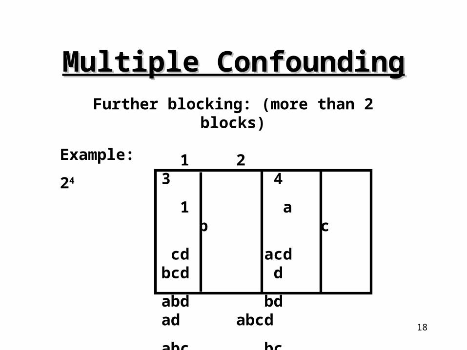
Multiple ConfoundingMultiple ConfoundingFurther blocking: (more than 2 blocks)

Example:

24

1 2 3 4

1 a b c

cd acd bcd d

abd bd ad abcd

abc bc ac ab

19

Imagine that these blocks differ by constants in terms of the variable being measured; all yields in the first block are too high (or too

low) by R. Similarly, the other 3 blocks are too high (or too low) by amounts S, T, U,

respectively. (These letters play the role of X in 2 - block confounding).

(R + S + T + U = 0 by definition)

20

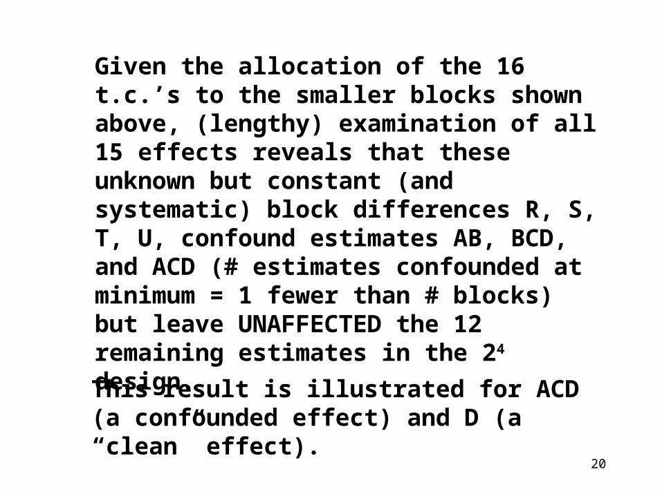
Given the allocation of the 16 t.c.’s to the smaller blocks shown above, (lengthy) examination of all 15 effects reveals that these unknown but constant (and systematic) block differences R, S, T, U, confound estimates AB, BCD, and ACD (# estimates confounded at minimum = 1 fewer than # blocks) but leave UNAFFECTED the 12 remaining estimates in the 24 design.

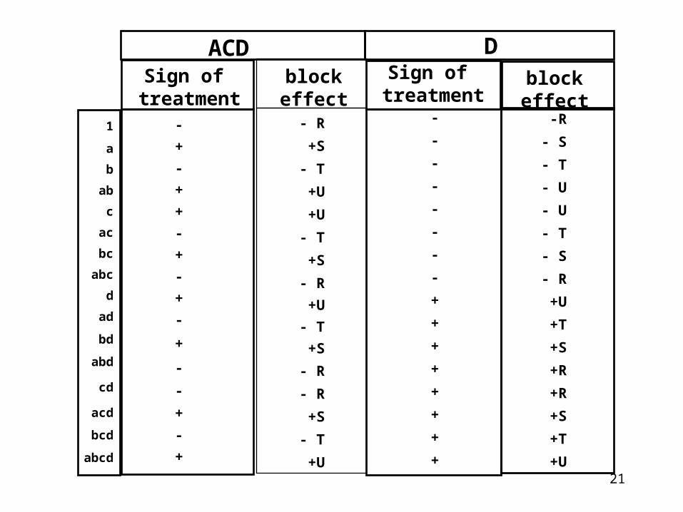
This result is illustrated for ACD (a confounded effect) and D (a “clean” effect).

21

Sign of treatment

Sign of treatment

block effect

block effect

1

a

b

ab

c

ac

bc

abc

d

ad

bd

abd

cd

acd

bcd

abcd

-

+

-

+

+

-

+

-

+

-

+

-

-

+

-

+

- R

+S

- T

+U

+U

- T

+S

- R

+U

- T

+S

- R

- R

+S

- T

+U

-

-

-

-

-

-

-

-

+

+

+

+

+

+

+

+

-R

- S

- T

- U

- U

- T

- S

- R

+U

+T

+S

+R

+R

+S

+T

+U

ACD D

22

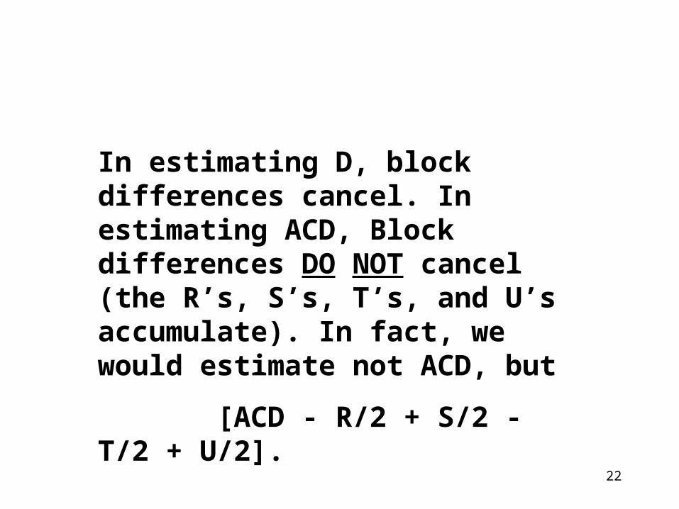
In estimating D, block differences cancel. In estimating ACD, Block differences DO NOT cancel (the R’s, S’s, T’s, and U’s accumulate). In fact, we would estimate not ACD, but

[ACD - R/2 + S/2 - T/2 + U/2].

23

The ACD estimate is hopelessly confounded with block effects.

We began this discussion of multiple Confounding with 4 treatment combo’s allocated to each of the four smaller blocks. We then determined what effects were and were not confounded.

24

Sensibly, this is ALWAYS REVERSED. The experimenter decides what effects he/she is willing to confound, then determines the treatments appropriate to each smaller block. (In our example, experimenter chose AB, BCD, ACD).

25

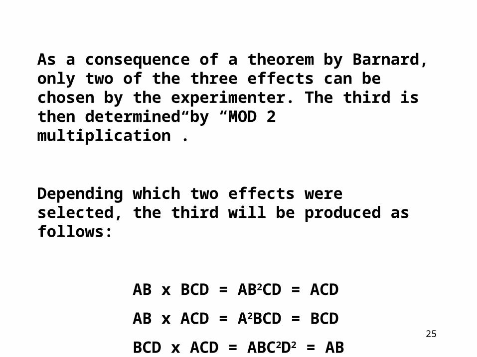
As a consequence of a theorem by Barnard, only two of the three effects can be chosen by the experimenter. The third is then determined by “MOD 2 multiplication”.

Depending which two effects were selected, the third will be produced as follows:

AB x BCD = AB2CD = ACD

AB x ACD = A2BCD = BCD

BCD x ACD = ABC2D2 = AB

26

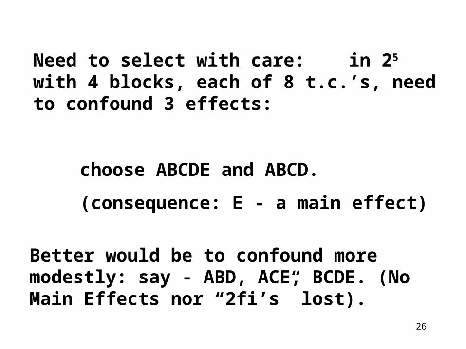
Need to select with care: in 25 with 4 blocks, each of 8 t.c.’s, need to confound 3 effects:

choose ABCDE and ABCD.

(consequence: E - a main effect)

Better would be to confound more modestly: say - ABD, ACE, BCDE. (No Main Effects nor “2fi’s” lost).

27

Once effects to be confounded are selected, t.c’s which go into each block are found as follows:

Those t.c.’s with an even number of letters in common with all confounded effects go into one block (the principal block); t.c.’s for the remaining block(s) are determined by MOD - 2 multiplication of the principal block.

28

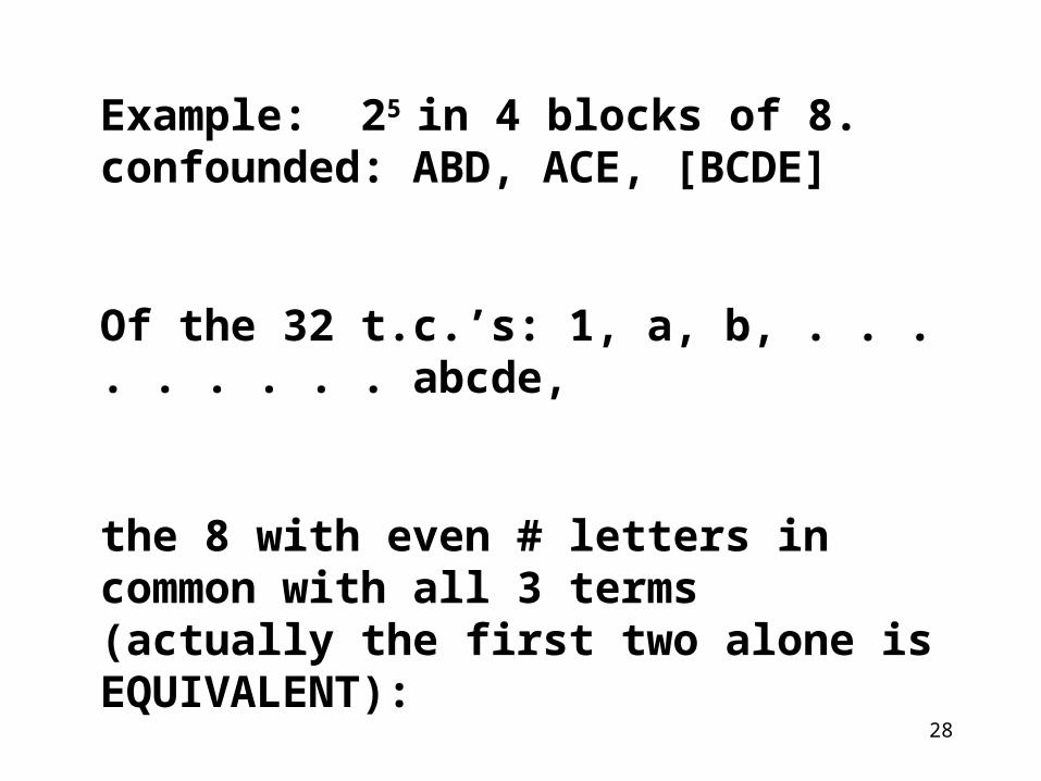
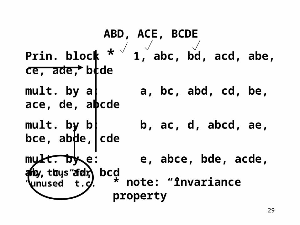
Example: 25 in 4 blocks of 8. confounded: ABD, ACE, [BCDE]

Of the 32 t.c.’s: 1, a, b, . . . . . . . . . abcde,

the 8 with even # letters in common with all 3 terms (actually the first two alone is EQUIVALENT):

29

Prin. block * 1, abc, bd, acd, abe, ce, ade, bcde

mult. by a: a, bc, abd, cd, be, ace, de, abcde

mult. by b: b, ac, d, abcd, ae, bce, abde, cde

mult. by e: e, abce, bde, acde, ab, c, ad, bcd

any thus far “unused” t.c. * note: “invariance property”

ABD, ACE, BCDE

30

Remember that we compute the 31 effects in the usual way. Only, ABD, ACE, BCDE are not “clean”. Consider from the 25 table of signs: P. 265, Tale 9.4.

31

If the influence of the unknown block effect, R, is to be removed, it must be done in Block 1, for R appears only in Block 1. You can see when it cancels & when it doesn’t.

(Similarly for S, T, U).

32

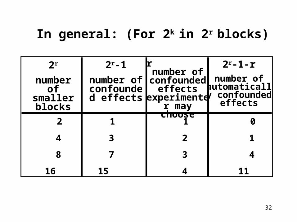
In general: (For 2k in 2r blocks)

2r

number of smaller blocks

2r-1

number of confounded

effects

r number of

confounded effects

experimenter may choose

2r-1-r

number of automatically confounded

effects

2

4

8

16

1

3

7

15

1

2

3

4

0

1

4

11

33

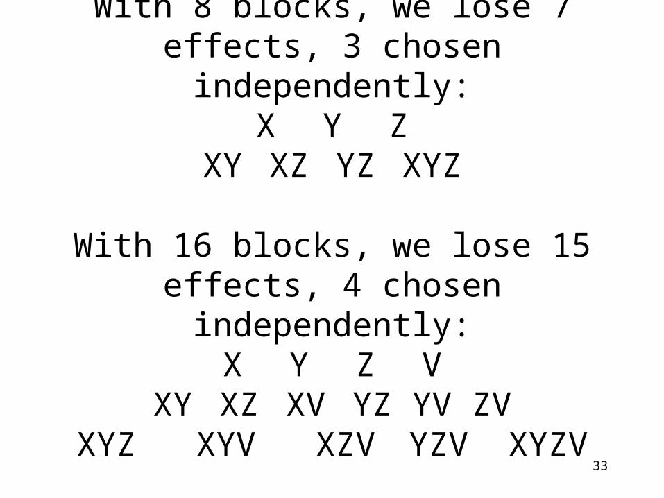
With 8 blocks, we lose 7 effects, 3 chosen independently:

X Y ZXY XZ YZ XYZ

With 16 blocks, we lose 15 effects, 4 chosen independently:

X Y Z VXY XZ XV YZ YV ZV

XYZ XYV XZV YZV XYZV

34

It may appear that there would be little interest in designs which confound as many as, say, 7 effects. Wrong! Recall that in a, say, 26, there’s 63=26-1 effects. Confounding 7 of 63 might well be tolerable.

35

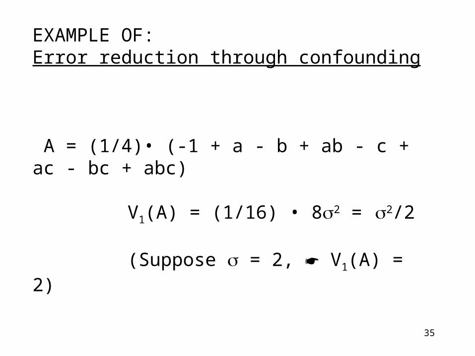
EXAMPLE OF: Error reduction through confounding

A = (1/4)• (-1 + a - b + ab - c + ac - bc + abc)

V1(A) = (1/16) • 82 = 2/2

(Suppose = 2, V1(A) = 2)

36

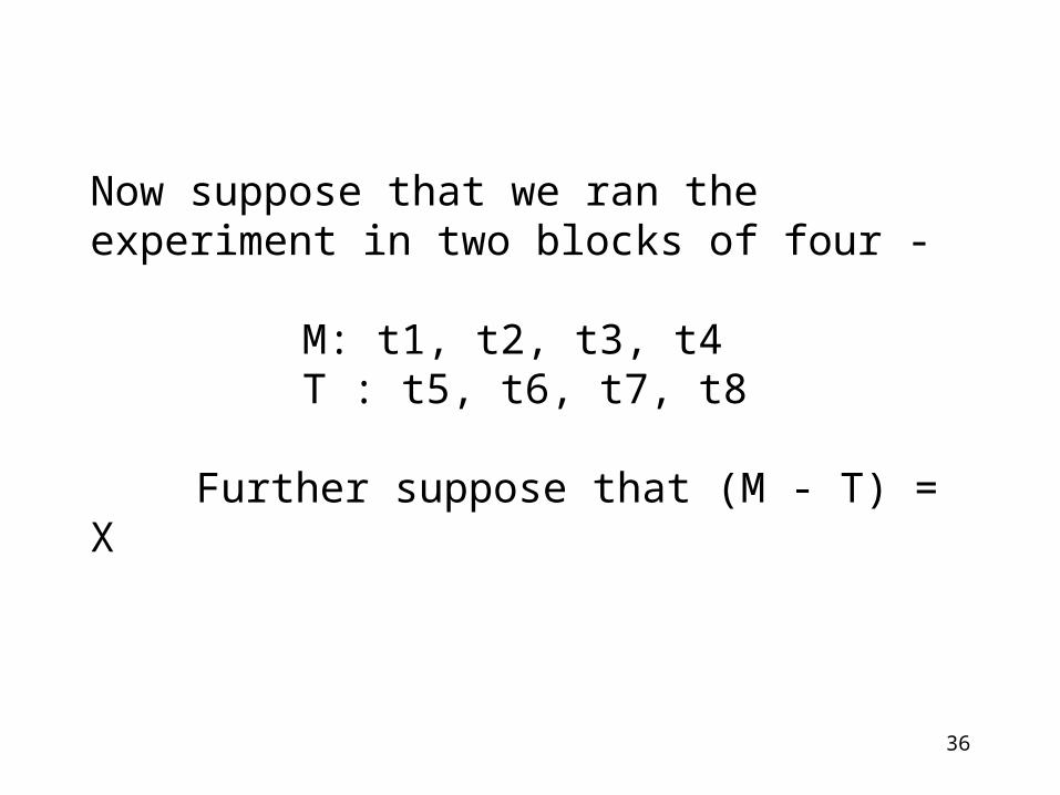
Now suppose that we ran the experiment in two blocks of four -

M: t1, t2, t3, t4T : t5, t6, t7, t8

Further suppose that (M - T) = X

37

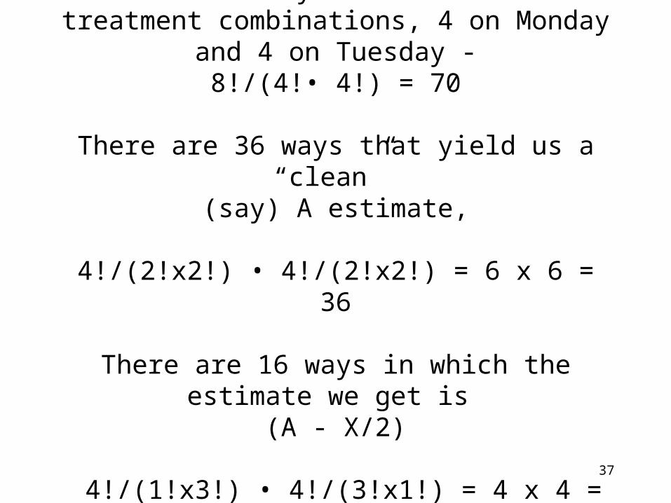
There are 70 ways to allocate the 8 treatment combinations, 4 on Monday and 4 on Tuesday -

8!/(4!• 4!) = 70

There are 36 ways that yield us a “clean” (say) A estimate,

4!/(2!x2!) • 4!/(2!x2!) = 6 x 6 = 36

There are 16 ways in which the estimate we get is (A - X/2)

4!/(1!x3!) • 4!/(3!x1!) = 4 x 4 = 16

38

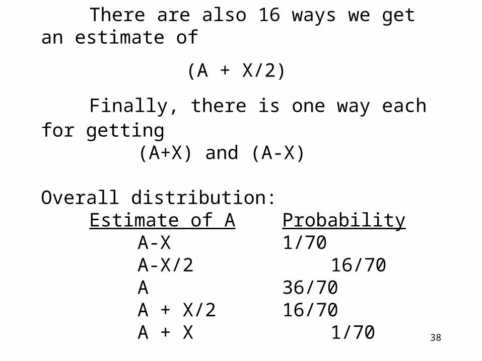
There are also 16 ways we get an estimate of

(A + X/2) Finally, there is one way each for getting

(A+X) and (A-X)

Overall distribution:Estimate of A Probability

A-X 1/70A-X/2 16/70A 36/70A + X/2 16/70A + X 1/70

39

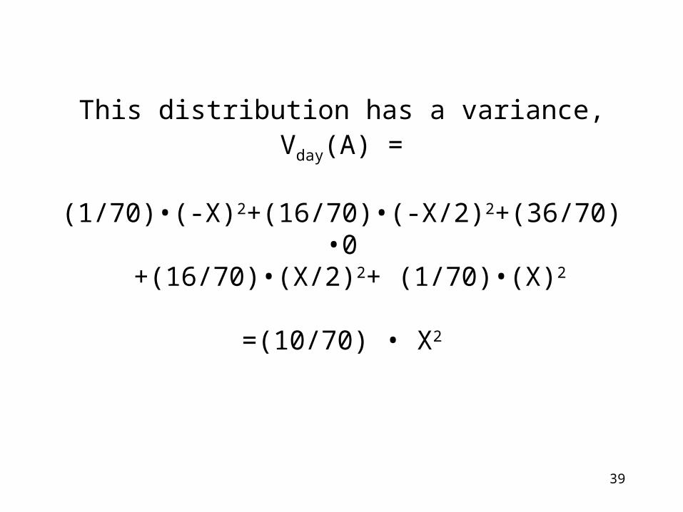
This distribution has a variance, Vday(A) =

(1/70)•(-X)2+(16/70)•(-X/2)2+(36/70)•0 +(16/70)•(X/2)2+ (1/70)•(X)2

=(10/70) • X2

40

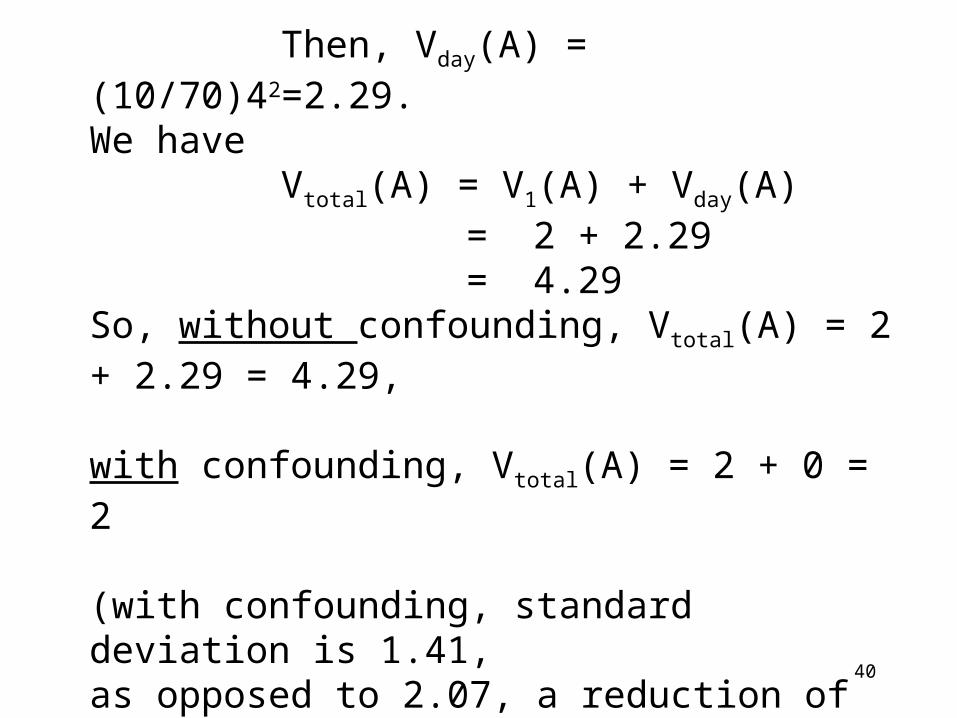
Suppose, for example, that X =4, same as 2.

Then, Vday(A) = (10/70)42=2.29.We have Vtotal(A) = V1(A) + Vday(A)

= 2 + 2.29 = 4.29

So, without confounding, Vtotal(A) = 2 + 2.29 = 4.29,

with confounding, Vtotal(A) = 2 + 0 = 2

(with confounding, standard deviation is 1.41, as opposed to 2.07, a reduction of 32%.)