1 Compositional models for audio processing

1

Compositional models for audio processing

Tuomas Virtanen, Jort F. Gemmeke, Bhiksha Raj, Paris Smaragdis

INTRODUCTION

Many classes of data are composed as constructive combinations of parts. By ”constructive” combination, we mean

additive combination that do not result in subtraction or diminishment of any of the parts. We will refer to such data

as “compositional” data. Typical examples include population or counts data, where the total count of a population

is obtained as the sum of counts of subpopulations. In order to characterize such data, a variety of mathematical

models have been developed in the literature which, in conformance with the nature of the data, represent them as

non-negative linear combinations of parts which themselves are also non-negative, to ensure that such combination

does not result in subtraction or diminishment. We will refer to such models as “compositional” models.

Although the notion of purely constructive composition most obviously applies to non-signal data such as counts of

populations, compositional models have frequently been employed to explain other forms of data as well [1]. During

the last few years such models have provided new paradigms to solve old standing audio processing problems, e.g.

blind and supervised source separation [2], [3], and robust recognition [4]. Therefore the models have been used

as parts of audio processing systems to advance the state of the art on many problems that deal with audio data

consisting of multiple sources, for example on the analysis of polyphonic music [5] and recognition of noisy speech

[6]. A significant reason to study these methods is not just their inherent robustness, but also the flexibility to use

them in ways which are non-standard in audio processing. In this paper we show how they can be powerful tools

for processing audio data, providing highly interpretable audio representations, and enabling diverse applications

such as signal analysis and recognition [7], [8], [4], manipulation and enhancement [9], [10], and coding [11], [12].

The basic premise underlying the application of compositional models to audio processing is that sound, too, can

be viewed as being compositional in nature. The premise has intuitive appeal: sound, as we experience it, does

indeed have compositional character. The sounds we hear are usually a medley of component sounds that are all

concurrently present. Although a sound may mask others by its greater prominence, the sounds themselves do

not generally cancel one another, except in few cases when it is done intentionally, for example in adaptive noise

cancellers. Even sounds produced by a single source are often compositions of component sounds from the source,

e.g. the sound produced by a machine combines sounds from all its parts, and music sounds are compositions of

notes produced by the various instruments.

The compositionality of sound is also evident in time-frequency characterizations of the signal, as illustrated by

November 17, 2014 DRAFT

2

time (s)

freq

uenc

y (k

Hz)

magnitude spectrogram

1 2 30

0.5

1

1.5

2

2.5

3

3.5

4

4.5

5

0.1

0.2

0.3

0.4

0.5

0.6

0.7

0.8

0.9

1

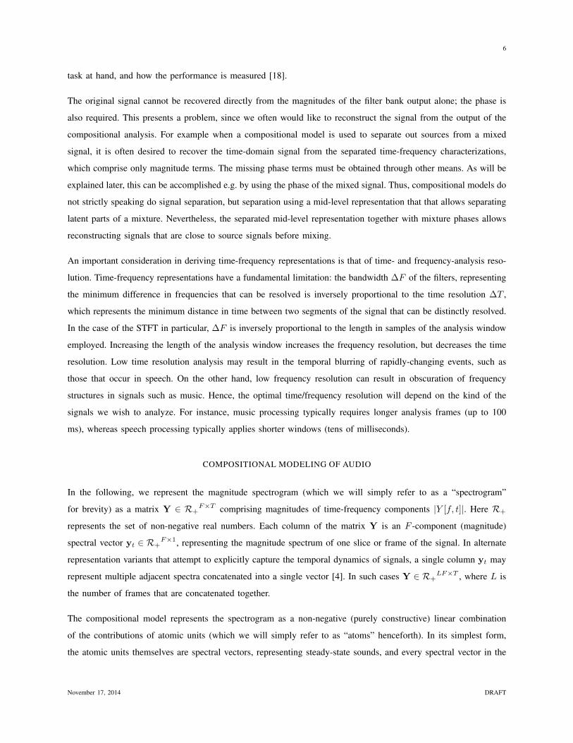
Fig. 1. A magnitude spectrogram of a simple piano recording. Two notes are played in succession and then again in unison. We can visually

identify these notes using their unique harmonic structure.

Figure 1. The figure shows a spectrogram – a visual representation of the magnitude of time-frequency components

as a function of time and frequency – of a signal which comprises two notes played individually at first and then

played together. The spectral patterns characteristic of the individual notes are distinctly observable even when they

are played together.

The compositional framework for sound analysis builds upon these impressions: it characterizes the sounds from

any source as a constructive composition of atomic sounds that are characteristic of the source, and postulates that

the decomposition of the signal into its atomic parts may be achieved through the application of an appropriately

constrained compositional model to an appropriate time-frequency representation of the signal. This, in-turn, can

be utilized to perform several of the tasks mentioned earlier.

The models themselves may take multiple forms. The non-negative matrix factorization (NMF) models [3], [13]

treat non-negative time-frequency representations of the signal as matrices, which are decomposed into products of

non-negative component matrices. One of the matrices represent spectral patterns of the atomic parts, and other their

activation to the signal over time. The probabilistic latent component analysis (PLCA) models treat the non-negative

time-frequency representations as histograms drawn from a mixture of multi-variate multinomial random variables

representing the atomic parts [14]. The two approaches can be shown to be equivalent, and in fact arithmetically

identical under some circumstances [15].

The purpose of this article is to serve as an introduction to the application of compositional models to the analysis


3

of sound. We first demonstrate the limitations of related algorithms that allow cancellation of parts, and how

compositional models can circumvent them, through an example. We then continue with a brief exposition on the

type of time-frequency representations where compositional models may naturally be applied. We will subsequently

explain the models themselves. Two most common formulations of compositional models are based on matrix

factorization and PLCA. For brevity, we will primarily present the matrix factorization perspective, although we

will also introduce the PLCA model briefly for completeness. Within these frameworks we will address various

issues, including how a given sound may be decomposed into the contributions of its atomic parts, how the parts

themselves may be found, restrictions of the model vis-a-vis the number and nature of these parts and of the

decomposition itself, and finally how the solutions to these problems make various applications possible.

WHY CONSTRUCTIVE COMPOSITION

Before proceeding further, it may be useful to address a question that may already have struck the reader: since the

models themselves are effectively matrix decompositions, what makes the compositional model with its constraints

on purely constructive composition different from other forms of matrix decompositions such as principal component

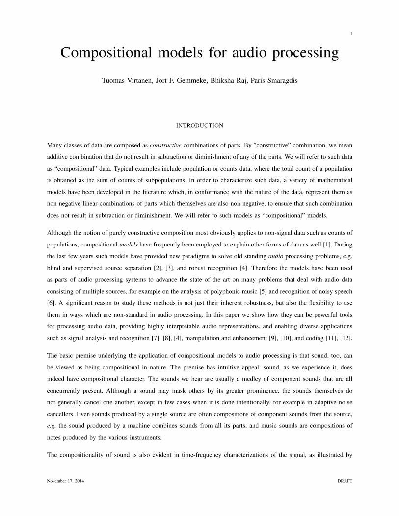
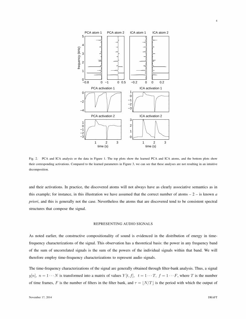
analysis (PCA), independent component analysis (ICA) or other similar methods? The answer is illustrated by Figure

2, which shows the outcome of PCA and ICA based decomposition of the spectrogram of Figure 1. Intuitively, the

signal is entirely composed of only two notes, and an effective decomposition technique would “discover” these

notes and when they were played. PCA and ICA were employed to decompose the spectrogram into two “bases”

and their activations. In both cases a nearly perfect decomposition is achieved, in the sense that the bases, when

excited by their corresponding activations, combine to construct the original spectrogram nearly perfectly, reflecting

the fact that the signal does indeed comprise only two basic elements (namely the two notes). However, inspection

of the actual bases discovered and their activations reveals a problem. PCA (illustrated by the panels to the left)

“discovers” two bases that, although orthogonal to one another, are actually combinations of the two notes, and their

corresponding activations provide no indication of the actual composition of the sound. In this particular example

ICA (illustrated by the panels to the right) does discover two bases whose activations do track the actual activation

of the notes in the signal. However the discovered bases themselves have both negative and positive components,

effectively characterizing the atomic units that compose the sound as having negative spectral magnitudes, which

has no physical interpretation. More generally, even the degree of conformance to the underlying structure found

in this particular example is usually not achieved. The intuitive dissonance is obvious – intuitively, the “building-

blocks” of this sound were the notes, and both methods have failed to discover these effectively. Although we do

not go into this further, the dissonance is more than intuitive; several of the solutions we develop later in the paper

through compositional models are simply not possible through normal matrix decomposition techniques such as

PCA and ICA that permit both constructive and destructive composition.

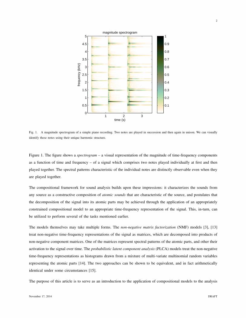
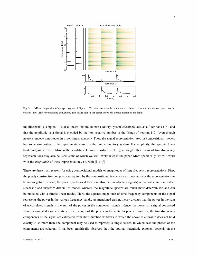
In contrast, Figure 3 shows the results obtained by decomposing the spectrogram of Figure 1 with NMF. The non-

negative factorization is observed to successfully uncover both, the notes themselves (as defined by their spectra)


4

0

1

2

3

4

5

−0.8 0

PCA atom 1

freq

uenc

y (k

Hz)

−1 0 0.5

PCA atom 2

−4

−2

0PCA activation 1

1 2 3

−3−2−1

01

PCA activation 2

time (s)

−0.2 0

ICA atom 1

0 0.2

ICA atom 2

−3−2−1

01

ICA activation 1

1 2 3

0

1

2

3ICA activation 2

time (s)

Fig. 2. PCA and ICA analysis or the data in Figure 1. The top plots show the learned PCA and ICA atoms, and the bottom plots show

their corresponding activations. Compared to the learned parameters in Figure 3, we can see that these analyses are not resulting in an intuitive

decomposition.

and their activations. In practice, the discovered atoms will not always have as clearly associative semantics as in

this example; for instance, in this illustration we have assumed that the correct number of atoms – 2 – is known a

priori, and this is generally not the case. Nevertheless the atoms that are discovered tend to be consistent spectral

structures that compose the signal.

REPRESENTING AUDIO SIGNALS

As noted earlier, the constructive compositionality of sound is evidenced in the distribution of energy in time-

frequency characterizations of the signal. This observation has a theoretical basis: the power in any frequency band

of the sum of uncorrelated signals is the sum of the powers of the individual signals within that band. We will

therefore employ time-frequency characterizations to represent audio signals.

The time-frequency characterizations of the signal are generally obtained through filter-bank analysis. Thus, a signal

y[n], n = 1 · · ·N is transformed into a matrix of values Y [t, f ], t = 1 · · ·T, f = 1 · · ·F , where T is the number

of time frames, F is the number of filters in the filter bank, and τ = bN/T c is the period with which the output of


5

0

1

2

3

4

5atom 1

freq

uenc

y (k

Hz)

atom 2

0.5 1 1.5 2 2.5 3 3.50

0.5

activation 2

time (s)

0

0.5

activation 1

approximation to input

Fig. 3. NMF decomposition of the spectrogram of Figure 1. The two panels on the left show the discovered atoms, and the two panels on the

bottom show their corresponding activations. The image plot in the center shows the approximation to the input.

the filterbank is sampled. It is also known that the human auditory system effectively acts as a filter bank [16], and

that the amplitude of a signal is encoded by the non-negative number of the firings of neurons [17] (even though

neurons encode amplitudes in a non-linear manner). Thus, the signal representation used in compositional models

has some similarities to the representation used in the human auditory system. For simplicity, the specific filter-

bank analysis we will utilize is the short-time Fourier transform (STFT), although other forms of time-frequency

representations may also be used, some of which we will invoke later in the paper. More specifically, we will work

with the magnitude of these representations, i.e. with |Y [t, f ]|.

There are three main reasons for using compositional models on magnitudes of time-frequency representations. First,

the purely constructive composition required by the compositional framework also necessitates the representations to

be non-negative. Second, the phase spectra (and therefore also the time-domain signals) of natural sounds are rather

stochastic and therefore difficult to model, whereas the magnitude spectra are much more deterministic and can

be modeled with a simple linear model. Third, the squared magnitude of time-frequency components of the signal

represents the power in the various frequency bands. As mentioned earlier, theory dictates that the power in the sum

of uncorrelated signals is the sum of the power in the component signals. Hence, the power in a signal composed

from uncorrelated atomic units will be the sum of the power in the units. In practice however, the time-frequency

components of the signal are estimated from short-duration windows in which the above relationship does not hold

exactly. Also more than one component may be used to represent a single source, in which case the phases of the

components are coherent. It has been empirically observed that, the optimal magnitude exponent depends on the


6

task at hand, and how the performance is measured [18].

The original signal cannot be recovered directly from the magnitudes of the filter bank output alone; the phase is

also required. This presents a problem, since we often would like to reconstruct the signal from the output of the

compositional analysis. For example when a compositional model is used to separate out sources from a mixed

signal, it is often desired to recover the time-domain signal from the separated time-frequency characterizations,

which comprise only magnitude terms. The missing phase terms must be obtained through other means. As will be

explained later, this can be accomplished e.g. by using the phase of the mixed signal. Thus, compositional models do

not strictly speaking do signal separation, but separation using a mid-level representation that that allows separating

latent parts of a mixture. Nevertheless, the separated mid-level representation together with mixture phases allows

reconstructing signals that are close to source signals before mixing.

An important consideration in deriving time-frequency representations is that of time- and frequency-analysis reso-

lution. Time-frequency representations have a fundamental limitation: the bandwidth ∆F of the filters, representing

the minimum difference in frequencies that can be resolved is inversely proportional to the time resolution ∆T ,

which represents the minimum distance in time between two segments of the signal that can be distinctly resolved.

In the case of the STFT in particular, ∆F is inversely proportional to the length in samples of the analysis window

employed. Increasing the length of the analysis window increases the frequency resolution, but decreases the time

resolution. Low time resolution analysis may result in the temporal blurring of rapidly-changing events, such as

those that occur in speech. On the other hand, low frequency resolution can result in obscuration of frequency

structures in signals such as music. Hence, the optimal time/frequency resolution will depend on the kind of the

signals we wish to analyze. For instance, music processing typically requires longer analysis frames (up to 100

ms), whereas speech processing typically applies shorter windows (tens of milliseconds).

COMPOSITIONAL MODELING OF AUDIO

In the following, we represent the magnitude spectrogram (which we will simply refer to as a “spectrogram”

for brevity) as a matrix Y ∈ R+F×T comprising magnitudes of time-frequency components |Y [f, t]|. Here R+

represents the set of non-negative real numbers. Each column of the matrix Y is an F -component (magnitude)

spectral vector yt ∈ R+F×1, representing the magnitude spectrum of one slice or frame of the signal. In alternate

representation variants that attempt to explicitly capture the temporal dynamics of signals, a single column yt may

represent multiple adjacent spectra concatenated into a single vector [4]. In such cases Y ∈ R+LF×T , where L is

the number of frames that are concatenated together.

The compositional model represents the spectrogram as a non-negative (purely constructive) linear combination

of the contributions of atomic units (which we will simply refer to as “atoms” henceforth). In its simplest form,

the atomic units themselves are spectral vectors, representing steady-state sounds, and every spectral vector in the


7

spectrogram can be decomposed into a non-negative linear combination of these atoms. We describe two formalisms

to achieve this decomposition.

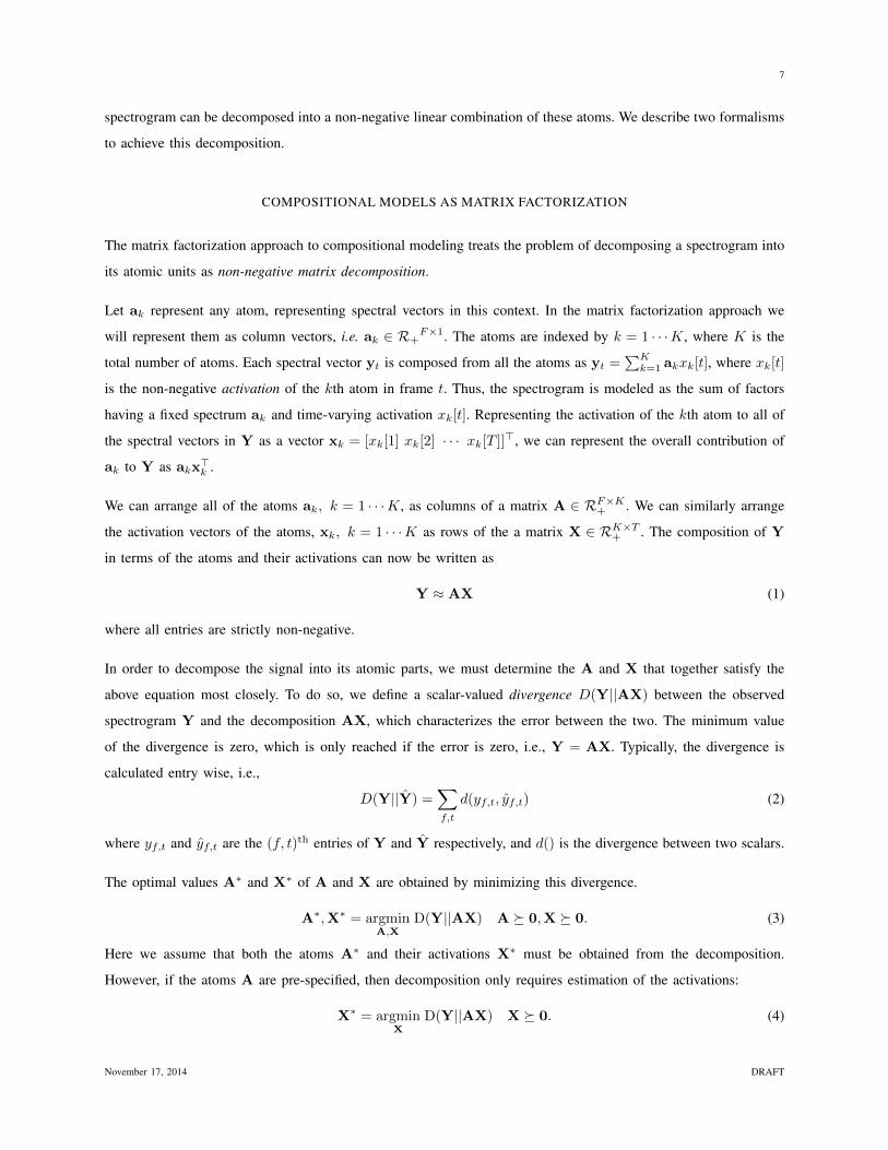
COMPOSITIONAL MODELS AS MATRIX FACTORIZATION

The matrix factorization approach to compositional modeling treats the problem of decomposing a spectrogram into

its atomic units as non-negative matrix decomposition.

Let ak represent any atom, representing spectral vectors in this context. In the matrix factorization approach we

will represent them as column vectors, i.e. ak ∈ R+F×1. The atoms are indexed by k = 1 · · ·K, where K is the

total number of atoms. Each spectral vector yt is composed from all the atoms as yt =∑Kk=1 akxk[t], where xk[t]

is the non-negative activation of the kth atom in frame t. Thus, the spectrogram is modeled as the sum of factors

having a fixed spectrum ak and time-varying activation xk[t]. Representing the activation of the kth atom to all of

the spectral vectors in Y as a vector xk = [xk[1] xk[2] · · · xk[T ]]>, we can represent the overall contribution of

ak to Y as akx>k .

We can arrange all of the atoms ak, k = 1 · · ·K, as columns of a matrix A ∈ RF×K+ . We can similarly arrange

the activation vectors of the atoms, xk, k = 1 · · ·K as rows of the a matrix X ∈ RK×T+ . The composition of Y

in terms of the atoms and their activations can now be written as

Y ≈ AX (1)

where all entries are strictly non-negative.

In order to decompose the signal into its atomic parts, we must determine the A and X that together satisfy the

above equation most closely. To do so, we define a scalar-valued divergence D(Y||AX) between the observed

spectrogram Y and the decomposition AX, which characterizes the error between the two. The minimum value

of the divergence is zero, which is only reached if the error is zero, i.e., Y = AX. Typically, the divergence is

calculated entry wise, i.e.,

D(Y||Y) =∑f,t

d(yf,t, yf,t) (2)

where yf,t and yf,t are the (f, t)th entries of Y and Y respectively, and d() is the divergence between two scalars.

The optimal values A∗ and X∗ of A and X are obtained by minimizing this divergence.

A∗,X∗ = argminA,X

D(Y||AX) A � 0,X � 0. (3)

Here we assume that both the atoms A∗ and their activations X∗ must be obtained from the decomposition.

However, if the atoms A are pre-specified, then decomposition only requires estimation of the activations:

X∗ = argminX

D(Y||AX) X � 0. (4)


8

0 0.5 1 1.5 20

0.2

0.4

0.6

0.8

1

1.2

1.4

1.6

1.8

2

y

d(y,y)

0 1 2 3 40

0.2

0.4

0.6

0.8

1

1.2

1.4

1.6

1.8

2

y

d(y,y)

squaredKLIS

squaredKLIS

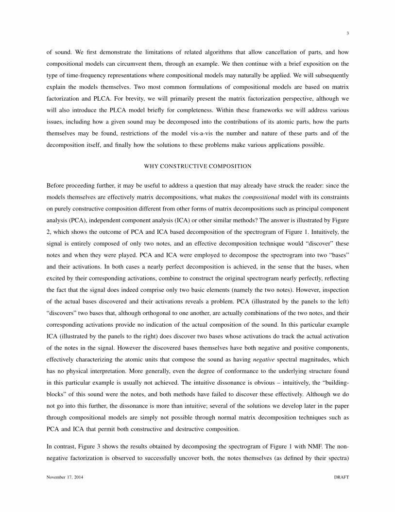
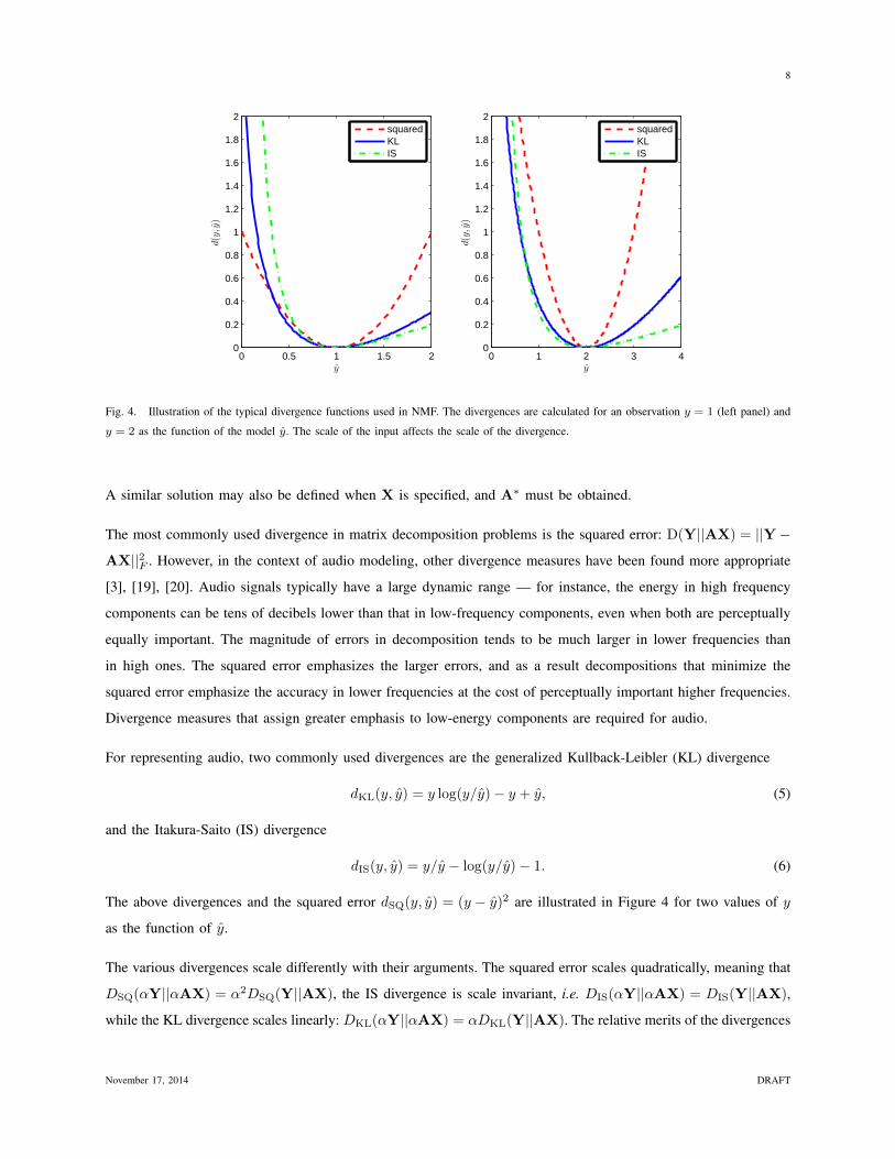
Fig. 4. Illustration of the typical divergence functions used in NMF. The divergences are calculated for an observation y = 1 (left panel) and

y = 2 as the function of the model y. The scale of the input affects the scale of the divergence.

A similar solution may also be defined when X is specified, and A∗ must be obtained.

The most commonly used divergence in matrix decomposition problems is the squared error: D(Y||AX) = ||Y−

AX||2F . However, in the context of audio modeling, other divergence measures have been found more appropriate

[3], [19], [20]. Audio signals typically have a large dynamic range — for instance, the energy in high frequency

components can be tens of decibels lower than that in low-frequency components, even when both are perceptually

equally important. The magnitude of errors in decomposition tends to be much larger in lower frequencies than

in high ones. The squared error emphasizes the larger errors, and as a result decompositions that minimize the

squared error emphasize the accuracy in lower frequencies at the cost of perceptually important higher frequencies.

Divergence measures that assign greater emphasis to low-energy components are required for audio.

For representing audio, two commonly used divergences are the generalized Kullback-Leibler (KL) divergence

dKL(y, y) = y log(y/y)− y + y, (5)

and the Itakura-Saito (IS) divergence

dIS(y, y) = y/y − log(y/y)− 1. (6)

The above divergences and the squared error dSQ(y, y) = (y − y)2 are illustrated in Figure 4 for two values of y

as the function of y.

The various divergences scale differently with their arguments. The squared error scales quadratically, meaning that

DSQ(αY||αAX) = α2DSQ(Y||AX), the IS divergence is scale invariant, i.e. DIS(αY||αAX) = DIS(Y||AX),

while the KL divergence scales linearly: DKL(αY||αAX) = αDKL(Y||AX). The relative merits of the divergences


9

may be inferred from this property: the squared error divergence puts undue emphasis on high-energy components

and the IS divergence fails to distinguish between the noise floor and higher-energy speech components. The KL

divergence provides a good compromise between the two [3], [19], [20]. A generalization of the above divergences

is the beta divergence [21], which defines a set of divergences that are a function of a parameter β.

The above divergences (KL, IS, or squared) can be obtained from maximum likelihood estimation of the parameters,

when observed data is generated by a specific generative model (Poisson distribution, multiplicative Gamma noise,

or additive Gaussian noise) independently at each time-frequency point [13]. Even though some of these models

(e.g. the Poisson distribution) do not match well with the distribution of natural sounds, the statistical interpretation

allows incorporating a prior distributions for the parameters.

The squared error and KL divergence are convex as the function of y, and for these, the divergence D(Y||Y) is

also convex in Y. In this case the optimization problem of Equations (4) and its counterpart, where X is specified

and A must be estimated, minimize a convex function and can be solved by any convex optimization technique.

When Y is itself a product of two matrices, e.g. Y = AX, D(Y||Y) = D(Y||AX) becomes biconvex in A and

X. This means means that it is not jointly convex in both of these variables, but if either of them is fixed it is

convex in the other. Therefore, Equation (3) is biconvex and cannot directly be solved through convex optimization

methods. Nevertheless, convex optimization methods may still be employed by alternately estimating one of A and

X, holding the other fixed to its current estimate.

A commonly used solution to estimating non-negative decompositions is based on so called multiplicative updates.

The parameters to be estimated are first initialized to random positive values, and then iteratively updated by

multiplying them with correction terms. The strength of the method stems from the ability of the updates to fulfill

the non-negativity constraints easily: provided that both the previous estimate and the correction term are non-

negative, the updated term is guaranteed to be non-negative as well. The multiplicative updates that decrease the

KL divergence are given as

A← A⊗YAXX>

1X>(7)

and

X← X⊗A> Y

AX

A>1, (8)

where 1 is an all-one matrix of the same size as Y, ⊗ is an element-wise matrix product, and all the divisions are

element wise. It can be easily seen that if A and X are non-negative, the terms that are used to update them are also

non-negative. Thus, the updates obey the non-negativity constraints. If both A and X must be estimated, Equations

(7) and (8) must be alternately computed. If one of the two is given and only the other must be estimated, then

only the update rule for the appropriate variable need be iterated. For instance, if A is given, X can be estimated

by iterating Equation (8). In all cases, the KL divergence is guaranteed be non-increasing under the updates. These

multiplicative updates and also rules for minimizing the squared error were proposed by Lee and Seung [22].


10

In addition to multiplicative updates, a variety of alternative methods have been proposed, based on e.g. second-

order methods [23], projected gradient [1, pp. 267-268], etc. The methods can also be accelerated by active-set

methods [24], [25]. Some divergences such as the IS divergence are not convex, and minimizing them requires

more carefully designed optimization algorithms than the convex divergences [13].

There also exist divergences that aim at optimizing the perceptual quality of the representation [12], which are

useful in audio coding applications. In most of the other applications of compositional models such as source

separation and signal analysis, however, the quality of the representation is affected more by its ability to isolate

latent compositional units from a mixture signal, not the ability to represent accurately the observations. Therefore,

simple divergences such as the KL or IS are the most commonly used even in the applications where a mixture is

separated into parts for listening purposes.

COMPOSITIONAL MODELS AS PROBABILISTIC LATENT COMPONENT ANALYSIS

The probabilistic latent component analysis (PLCA) approach to compositional models treats the spectrogram of the

signal as a histogram drawn from a mixture multinomial process, where the component multinomials in the mixture

represent the atoms that compose the signal [14]. This model is an extension of probabilistic latent semantic indexing

and probabilistic latent semantic analysis techniques that have been successfully used e.g. for topic modeling of

speech [26].

The generative model behind PLCA may be explained as follows. A stochastic process draws frequency indices

randomly from a collection of multinomial distributions. In each draw, it first selects one of these component

multinomials according to some probability distribution P (k), where k represents the selected multinomial. Subse-

quently, it draws the frequency f from the selected multinomial P (f |k). Thus, the probability that a frequency f

will be selected in any draw is given by∑k P (k)P (f |k). In order to generate a spectral vector the process draws

frequencies several times. The histogram of the frequencies is the resulting spectral vector.

The mixture multinomial∑k P (k)P (f |k) thus represents the distribution underlying a single spectral vector –

the vector itself is obtained through several draws from this distribution. When we employ the model to generate

an entire spectrogram comprising many spectral vectors, we make an additional assumption: that the component

multinomials P (f |k) are characteristic of the source that generates the sound, and represent the atomic units for

the source. Hence the set of component multinomials is the same for all vectors, and the only factor that changes

from analysis frame to analysis frame is the probability distribution over k, which specifies how the component

multinomials are chosen in any draw. The overall mixture multinomial distribution model for the spectrum of the

t-th analysis frame in the signal is given by

Pt(f) =

K∑k=1

Pt(k)P (f |k) (9)


11

where Pt(k) represents the frame-specific a priori probability of k in the t-th frame and P (f |k) represents the

multinomial distribution of f within the k-th atom. Even though the formulation of the model is different from

NMF, the models are conceptually similar: decomposition of a signal is equated to estimation of the atoms P (f |k)

and their activations Pt(k) to each frame of the signal, given the spectrogram Y [t, f ].

The estimation can be performed using the Expectation Maximization (EM) algorithm [27]. The various components

of the mixture multinomial distribution of Eq. (9) are initialized randomly and reestimated through iterations of the

following equations:

Pt(k|f) =Pt(k)P (f |k)∑K

k′=1 Pt(k′)P (f |k′)

P (f |k) =

∑Tt=1 Pt(k|f)Y [t, f ]∑T

t=1

∑Ff ′=1 Pt(k|f ′)Y [t, f ]

(10)

Pt(k) =

∑Ff=1 Pt(k|f)Y [t, f ]∑K

k′=1

∑Ff=1 Pt(k

′|f)Y [t, f ]. (11)

The contribution of the k-th atom to the overall signal is the expected number of draws from the multinomial for

the atom, given the observed spectrum and is given by

Yk[t, f ] = Y [t, f ]Pt(k|f) = Y [t, f ]Pt(k)P (f |k)∑K

k′=1 Pt(k′)P (f |k′)

.

This effectively distributes the intensity of Y [t, f ] using the posterior probability of the kth source in point [t, f ],

and is equivalent to the ”Wiener”-style reconstruction described in the next section.

The rest of this paper is presented primarily through the matrix-factorization perspective, for brevity. However many

of the NMF extensions described below are also possible within the PLCA framework, often in a manner that is

more mathematically intuitive than the matrix-factorization framework. These include e.g. tensor decompositions

[27], convolutive representations, the imposition of temporal constraints [28], joint recognition of mixed signals,

imputation of missing data [29], etc. We refer the reader to the above studies for additional details of these models.

UNIQUENESS, REGULARIZATION, AND SPARSITY

The solutions to Equations (3) and (4) are not always unique. We have noted that the divergence D(Y||AX) is

biconvex in A and X. As a result, when both A and X are to be estimated, multiple solutions may be obtained

that result in the same divergence. Specifically, for any Y ∈ RF×T+ , if (A ∈ RF×K+ , X ∈ RK×T+ ) is a solution

that minimizes the divergence, then any matrix pair (A ∈ RF×K+ , X ∈ RK×T+ ) such that AX = AX is also a

solution. For K ≥ F in particular, trivial solutions also become possible. For K = F , Y = AX can be made exact

by simply setting A = I and X = Y. For K > F , infinite exact decompositions may be found, for instance simply

by setting the the first F columns of A to the identity matrix; the remaining dictionary atoms become irrelevant

(and can be set to anything at all) as an exact decomposition can be obtained by setting their activations to 0.


12

Even if A is specified and only X must be estimated, the solution may not be unique although D(Y||AX) is

convex in X. This happens particularly when A is overcomplete, i.e. when K ≥ F . Any F linearly independent

columns of A can potentially be used to represent an F -dimensional vector with zero error. We can choose F

linearly-independent atoms from A ∈ RF×K+ in up to(KF

)ways, potentially giving us at least that many ways

of decomposing any vector in Y in terms of the atoms in A. If we permit combinations of more than F atoms,

the number of minimum-divergence decompositions of a vector in terms of A can be much greater. The exact

conditions for the uniqueness of the decompositions is studied in more detail in [30].

In order to reduce the ambiguity in the solution, it is customary to impose additional constraints on the decom-

position, which is typically done through “regularization” terms that are added to the divergence to be minimized.

Within the NMF framework, this modifies the optimization problem of Eq. (3) to

A∗,X∗ = argminA,X

D(Y||AX) + λΦ(X) A � 0,X � 0. (12)

where Φ(X) is a differentiable, scalar function of X whose value decreases as the conformance of X to the desired

constraint increases, and λ is a positive weight that is given for the regularization term.

Introduction of a regularization term as given above can nevertheless still result in trivial solutions. Two solutions

(A,X) and (A, X) will result in identical divergence values if A = ε−1A and X = εX, i.e. D(Y||AX) =

D(Y||AX). Structurally, the two solutions are identical since they are merely scaled versions of one another.

On the other hand, the regularization terms for the two need not be identical: Φ(X) 6= Φ(X). As a result, the

regularization term on the right hand side of Equation (12) can be minimized by simply scaling X by appropriate

ε values and scaling A up by ε−1, without actually modifying the decomposition obtained.

In order to avoid this problem, it becomes necessary to scale the atoms in A to have a constant `2 norm. Typically,

this is done by normalizing every atom ai in A such that ||ai||2 = 1 after every update. Assuming that all atoms

are normalized to unit `2 norm, for the KL divergence, the update rules from Eq. (8) is modified to

X← X⊗A> Y

AX

A>1 + λΦ′(X), (13)

where Φ′(X) is the matrix derivative of Φ(X) with respect to X. The update rule for A remains unchanged,

besides the additional requirement that atoms must be normalized after every iteration. There exists also ways to

take the normalization into account in the update, which guarantee that the updates and normalization together

decrease the value of the cost function [31], [3].

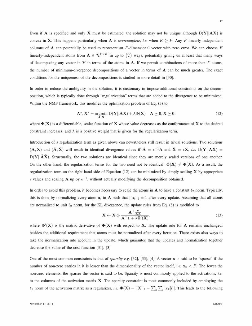
One of the most common constraints is that of sparsity e.g. [32], [33], [4]. A vector x is said to be “sparse” if the

number of non-zero entries in it is lesser than the dimensionality of the vector itself, i.e. x0 < F . The fewer the

non-zero elements, the sparser the vector is said to be. Sparsity is most commonly applied to the activations, i.e.

to the columns of the activation matrix X. The sparsity constraint is most commonly included by employing the

`1 norm of the activation matrix as a regularizer, i.e. Φ(X) = ||X||1 =∑k

∑t |xk[t]|. This leads to the following


13

update rule for the activations:

X← X⊗A> Y

AX

A>1 + λ. (14)

Other constraints may similarly be applied by modifying the regularization function Φ(X) to favor the type of

solutions desired. Similarly, regularization functions may be applied on dictionary A, in which case the update rule

of A should be modified. In the context of compositional models for audio, the types of regularizations applied on

the dictionary include sparsity [32] and dissimilarity between learned atoms and generic speech templates [34].

It must be noted that in spite of the introduction of regularization terms, both Equations (3) and (12) are still

typically biconvex, and no algorithm is guaranteed to reach the global minimum in practice. Different algorithms

and initializations lead to to different solutions, and any solution obtained will, at best, be a local optimum. In

practice, this can result in some degree of variation in the signal processing outcomes obtained through these

decompositions.

The entire discussion above also applies to the PLCA decompositions, although the manner in which the regu-

larization terms are applied within the PLCA framework is different. We refer the reader to [35], [14], [27] for

additional discussion of this topic.

SOURCE SEPARATION

Sound source separation refers to the problem of extracting a single or several signals of interest from a mixture

containing multiple signals. This operation is central to many signal processing applications, because the fundamental

algorithms are typically build under the assumption that we operate on a clean target signal with minimal interference.

Having the ability to remove unwanted components from a recording can allow us to perform subsequent operations

that expect a clean input (e.g. speech recognition, or pitch detection). We will predominantly focus on the case

where we only observe a single-channel mixture, and briefly discuss multi-channel approaches later in the paper.

The compositional model approach to separation of signals from single-channel recordings addresses the problem

in a rather simple manner. It assumes that any sound source can draw upon a characteristic set of atomic sounds

to generate signals. Here, a “source” can refer to an actual sound source, or to some other grouping of acoustic

phenomena that should be jointly modeled, such as background noise, or even a collection of sound classes that

must be distinguished from a target class. A mixture of signals from distinct sources is composed of atoms from

the individual sources. The separation of any particular component signal from a mixture hence only requires the

segregation of the contribution of the atoms from that source from the mixture.

Mathematically, we can explain this as follows. We use the NMF formulation in our explanation. Let matrix As

represent the set of atoms employed by the s-th source. We will refer to it as a dictionary of atoms for that source.

Any spectrogram Ys from the s-th source is composed from the atoms in the dictionary As as Ys = AsXs. A


14

mixed signal Ymix combining signals from several sources is given by

Ymix =∑s

Ys =∑s

AsXs (15)

Equation (15) can be written more compactly as follows. Let A = [A1A2 · · · ] be a matrix composed by stacking

the dictionaries for all the sources side by side. Let X =[X>1 X>2 · · ·

]>be a matrix composed by stacking the

activations for all the sources vertically. We can now express the mixed signal in compact form as

Ymix = AX

The contribution of the s-th source to Ymix is simply Ys = AsXs.

In unsupervised source separation, both A, X are estimated from the observation Ymix, followed by a process

which identifies which source each atom is predominantly associated with. In a supervised scenario for separation,

the dictionaries As for each of the sources are known a priori. We address the problem of creating these dictionaries

in the next section. Thus As ∀s are known, and thereby so is A. X can now be estimated through iterations of

Equation (8).

The activations X∗s of source s can be extracted from the estimated activation matrix X∗ by selecting the rows

corresponding to the atoms from the s-th source. The estimated spectrogram for the s-th source is then simply

computed as

Ys = AsX∗s (16)

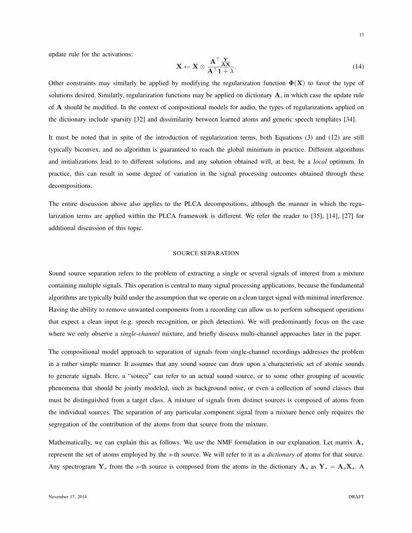
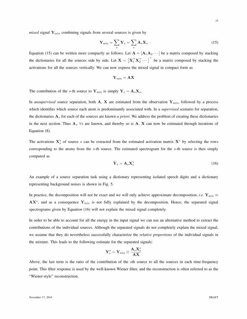
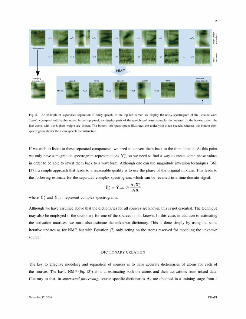
An example of a source separation task using a dictionary representing isolated speech digits and a dictionary

representing background noises is shown in Fig. 5.

In practice, the decomposition will not be exact and we will only achieve approximate decomposition, i.e. Ymix ≈

AX∗, and as a consequence Ymix is not fully explained by the decomposition. Hence, the separated signal

spectrograms given by Equation (16) will not explain the mixed signal completely.

In order to be able to account for all the energy in the input signal we can use an alternative method to extract the

contributions of the individual sources. Although the separated signals do not completely explain the mixed signal,

we assume that they do nevertheless successfully characterize the relative proportions of the individual signals in

the mixture. This leads to the following estimate for the separated signals:

Y∗s = Ymix ⊗AsX

∗s

AX

Above, the last term is the ratio of the contribution of the sth source to all the sources in each time-frequency

point. This filter response is used by the well-known Wiener filter, and the reconstruction is often referred to as the

“Wiener-style” reconstruction.


15

NMF

=xs1 +xs

2 +xs3 +xs

4 +xs5 +xs

6 ... +xsJ

+xn1 +xn

2 +xn3 +xn

4 +xn5 +xn

6 ... +xnK

0.2 +0.1 +0.09 +0.08 +0.08

noisylspeech

underlyingcleanlspeech

estimatedcleanlspeechspeech speech speechnoise noise

≈

clea

nlsp

eech

exem

plar

sno

ise

exem

plar

s

Fig. 5. An example of supervised separation of noisy speech. In the top left corner, we display the noisy spectrogram of the isolated word

“zero”, corrupted with babble noise. In the top panel, we display parts of the speech and noise exemplar dictionaries. In the bottom panel, the

five atoms with the highest weight are shown. The bottom left spectrogram illustrates the underlying clean speech, whereas the bottom right

spectrogram shows the clean speech reconstruction.

If we wish to listen to these separated components, we need to convert them back to the time domain. At this point

we only have a magnitude spectrogram representations Y∗s , so we need to find a way to create some phase values

in order to be able to invert them back to a waveform. Although one can use magnitude inversion techniques [36],

[37], a simple approach that leads to a reasonable quality is to use the phase of the original mixture. This leads to

the following estimate for the separated complex spectrogram, which can be reverted to a time-domain signal:

Y∗s = Ymix ⊗AsX

∗s

AX

where Y∗s and Ymix represent complex spectrograms.

Although we have assumed above that the dictionaries for all sources are known, this is not essential. The technique

may also be employed if the dictionary for one of the sources is not known. In this case, in addition to estimating

the activation matrices, we must also estimate the unknown dictionary. This is done simply by using the same

iterative updates as for NMF, but with Equation (7) only acting on the atoms reserved for modeling the unknown

source.

DICTIONARY CREATION

The key to effective modeling and separation of sources is to have accurate dictionaries of atoms for each of

the sources. The basic NMF (Eq. (3)) aims at estimating both the atoms and their activations from mixed data.

Contrary to that, in supervised processing, source-specific dictionaries As are obtained in a training stage from a


16

source-specific dataset, and combined to form the whole dictionary. The dictionary is then kept fixed and only the

activations are estimated according to Eq. (4).

There are two main approaches for dictionary learning: the first attempts to learn dictionary atoms which jointly

describe the training data [38], [39], whereas the second approach uses samples from the training data itself as

its dictionary atoms: a sampling based approach [35], [4]. Good dictionaries have several properties. They should

be capable of accurately describing the source, and generalize well to unseen data. They should be kept relatively

small, to reduce computational complexity. They should be discriminative, meaning that sources cannot be well

represented using a dictionary of another source. These requirements can be at odds with each other, for example

because small, accurate dictionaries are often less discriminative. The various approaches for dictionary creation

each have their strengths and weaknesses.

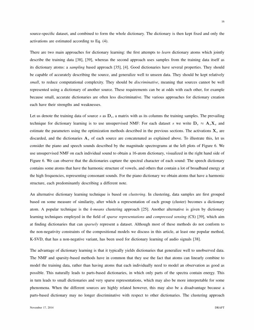
Let us denote the training data of source s as Ds, a matrix with as its columns the training samples. The prevailing

technique for dictionary learning is to use unsupervised NMF: For each dataset s we write Ds ≈ AsXs and

estimate the parameters using the optimization methods described in the previous sections. The activations Xs are

discarded, and the dictionaries As of each source are concatenated as explained above. To illustrate this, let us

consider the piano and speech sounds described by the magnitude spectrograms at the left plots of Figure 6. We

use unsupervised NMF on each individual sound to obtain a 16-atom dictionary, visualized in the right hand side of

Figure 6. We can observe that the dictionaries capture the spectral character of each sound: The speech dictionary

contains some atoms that have the harmonic structure of vowels, and others that contain a lot of broadband energy at

the high frequencies, representing consonant sounds. For the piano dictionary we obtain atoms that have a harmonic

structure, each predominantly describing a different note.

An alternative dictionary learning technique is based on clustering. In clustering, data samples are first grouped

based on some measure of similarity, after which a representation of each group (cluster) becomes a dictionary

atom. A popular technique is the k-means clustering approach [25]. Another alternative is given by dictionary

learning techniques employed in the field of sparse representations and compressed sensing (CS) [39], which aim

at finding dictionaries that can sparsely represent a dataset. Although most of these methods do not conform to

the non-negativity constraints of the compositional models we discuss in this article, at least one popular method,

K-SVD, that has a non-negative variant, has been used for dictionary learning of audio signals [38].

The advantage of dictionary learning is that it typically yields dictionaries that generalize well to unobserved data.

The NMF and sparsity-based methods have in common that they use the fact that atoms can linearly combine to

model the training data, rather than having atoms that each individually need to model an observation as good as

possible. This naturally leads to parts-based dictionaries, in which only parts of the spectra contain energy. This

in turn leads to small dictionaries and very sparse representations, which may also be more interpretable for some

phenomena. When the different sources are highly related however, this may also be a disadvantage because a

parts-based dictionary may no longer discriminative with respect to other dictionaries. The clustering approach


17

time (s)

freq

uenc

y (k

Hz)

speech magnitude spectrogram

1 2 30

1

2

3

4

5

5 10 150

1

2

3

4

5

atom index

learned speech dictionary

time (s)

freq

uenc

y (k

Hz)

piano magnitude spectrogram

1 2 30

1

2

3

4

5

5 10 150

1

2

3

4

5

atom index

learned piano dictionary

Fig. 6. Learning dictionaries from different sound classes. The top plots show an input magnitude spectrogram for a speech recording, and

the a dictionary that was extracted from it. The bottom plots show a piano recording input and its corresponding dictionary. Note how both

dictionaries capture salient spectral features from each sound.

typically yields dictionaries that are larger, but more discriminative.

While dictionary learning is a powerful method to create small dictionaries, it can be difficult to train overcomplete

dictionaries, in which there are many more atoms than features. A large number of atoms would naturally increase

the representation capability of the model, but learning overcomplete dictionaries from data then requires additional

constraints such as sparsity and careful tuning, as will be discussed in the next section. As an alternative to learning

the dictionaries representing training data, dictionary atoms can also be sampled from the data. Given a training

dataset Ds, the dictionary As is constructed as a subset of the columns of Ds.

By far the simplest method is random sampling, where the dictionary is formed by a random subset of columns

of Ds. Interestingly, dictionaries obtained with this approach yield comparable and often superior results as more

complex dictionary creation schemes [4]. The example in Figure 5 used a randomly sampled atoms representing


18

isolated speech digits and background noise.

The sampling methods have in common that they typically require little tuning and allow for the creation of large,

overcomplete dictionaries. A disadvantage is that they may not generalize as well to unseen data, and that smaller

dictionaries are often incapable of accurately modeling a source because they disregard the fact that atoms can

linearly combine to model an observation.

An alternative approach to dictionary creation, which avoids the need for training data, is to create dictionaries

by using prior knowledge of the structure of the signals. For example, in music transcription harmonic atoms

that represent different fundamental frequencies have been successfully used [8]. In the excitation-filter model [5],

described later in this article, atoms can describe filter-bank responses and excitations. This approach is only used

in a small number of specialized applications because while it yields small dictionaries that generalize well, they

are typically not very discriminative.

THE NUMBER OF ATOMS IN THE DICTIONARY

Let us now consider the issue of the number of atoms in the dictionary more carefully. Dictionary atoms are assumed

to represent basic atomic spectral structures that a sound source may produce. A source may produce any number

of distinct spectral structures. In order to accommodate all of them, the dictionary must ideally be large. When

we attempt to learn large dictionaries however, we run into a mathematical restriction: K becomes larger than F

and, as a result, in the absence of other restrictions, trivial solutions for A can be obtained as explained earlier.

Consequently, a learned dictionary with F or more atoms will generally be trivial, and carry little information about

the actual signal itself. Even if the dictionary is not learned through the decomposition, but specified through other

means such as through random draws from the training data, we run into difficulties when we attempt to explain

any spectral vector in terms of this dictionary. In the absence of other restrictions, the decomposition of an F × 1

spectral vector in terms of an F ×K dictionary is not unique when K ≥ F as explained earlier.

In order to overcome the non-uniqueness, additional constraints must be applied through appropriate regularization

terms. The most common constraint that is applied is that of sparsity. Sparsity is most commonly applied to the

activations, i.e. to the columns of the activation matrix X. Intuitively, this is equivalent to the claim that although

a source may draw from a large dictionary of atoms, any single spectral vector will only include a small number

of these. Other commonly applied constraints are group sparsity, promotes sparsity over groups of atoms [40], and

temporal continuity, which promotes smooth temporal variation of activations [3].

The number of atoms in the dictionary has great impact on the decomposition, even when the number of atoms is

less than F . Ideally the number atoms should equal the number of latent compositional units within the signal. In

certain cases we might know exactly what this number might be (e.g. when learning a dictionary for a synthetic

sound with a discrete number of states) but more commonly this information is not available and the number of


19

atoms in the dictionary must be determined in other ways. A dictionary with too few elements will be unable to

adequately explain all sounds from a given source, whereas one with too many elements may overgeneralize and

explain unintended sounds that do not belong to that source as well, rendering it ineffective for most processing

purposes. Although in principle the Bayesian Information Criterion (BIC) can be employed to automatically obtain

the optimal dictionary size, it is generally not as useful in this setting [41] and more sophisticated reasoning should

be used. Sparsity can be used for automatic estimation of the number of atoms, for example by initializing the

dictionary with a large number of atoms, enforcing sparsity on the activations, and reducing dictionary size by

eliminating all atoms that exhibit consistently low activations [42]. Another approach is to make use of Bayesian

formulations that allow for model selection in a natural way. For example the Markov chain Monte Carlo (MCMC)

methodology has been applied to estimate the size of a dictionary [41], [43].

In general, the trend is that larger dictionaries lead to better representations, and consequently superior signal

processing, e.g. in terms of the separation quality [25], provided that they are appropriately acquired. The downside

of larger dictionaries is of course increased computational complexity.

ANALYZING THE SEMANTICS OF SOUND

One of the fundamental goals in audio processing is the extraction of semantics from audio signals, with ample

applications such as music analysis, speech recognition, speaker identification, multi-media archive access and

audio event detection. The source separation applications described in the previous sections are often used as a

pre-processing step for conventional machine learning techniques used in audio analysis, such as Gaussian mixture

models (GMMs) and hidden Markov models (HMMs). The compositional model itself, however, is also a powerful

technique to extract meaning from audio signals and mixtures of audio signals.

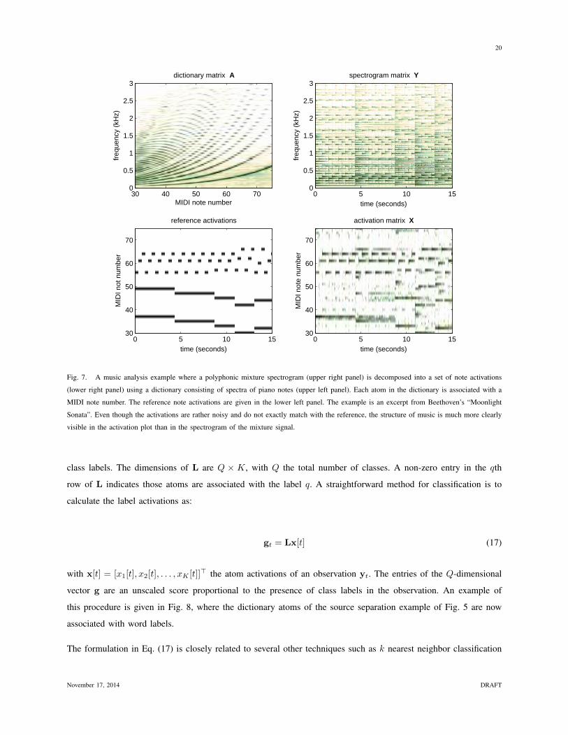
As an illustrating example, let us consider a music transcription task. The goal is to transcribe the score of a music

piece, that is, the pitch and duration of the sounds (notes) that are played. Even when considering a recording

in which only a single instrument such as a piano is playing, this is a challenging task since multiple notes can

be played at once. Moreover, although each note is characterized by a single fundamental frequency, their energy

may span the complete harmonic spectrum. These two aspects make music transcription difficult for conventional

methods based on sinusoidal modeling and STFT spectrum analysis, in which notes are associated with a single

frequency band, or machine learning methods, which cannot model overlapping notes. An example using NMF is

shown in Fig. 7.

Information extraction using the compositional model works by associating each atom in the dictionary with meta

information, for example class labels indicating notes. With the observation described as a linear combination of

atoms, the activation of these atoms then serves directly as evidence for the presence of (multiple) associated class

labels. Formally, let us define a label-matrix L, a binary matrix that associates each atom in A with one or multiple


20

MIDI note number

freq

uenc

y (k

Hz)

dictionary matrix A

30 40 50 60 700

0.5

1

1.5

2

2.5

3

time (seconds)

MID

I not

e nu

mbe

r

activation matrix X

0 5 10 1530

40

50

60

70

time (seconds)

MID

I not

num

ber

reference activations

0 5 10 1530

40

50

60

70

time (seconds)

freq

uenc

y (k

Hz)

spectrogram matrix Y

0 5 10 150

0.5

1

1.5

2

2.5

3

Fig. 7. A music analysis example where a polyphonic mixture spectrogram (upper right panel) is decomposed into a set of note activations

(lower right panel) using a dictionary consisting of spectra of piano notes (upper left panel). Each atom in the dictionary is associated with a

MIDI note number. The reference note activations are given in the lower left panel. The example is an excerpt from Beethoven’s “Moonlight

Sonata”. Even though the activations are rather noisy and do not exactly match with the reference, the structure of music is much more clearly

visible in the activation plot than in the spectrogram of the mixture signal.

class labels. The dimensions of L are Q × K, with Q the total number of classes. A non-zero entry in the qth

row of L indicates those atoms are associated with the label q. A straightforward method for classification is to

calculate the label activations as:

gt = Lx[t] (17)

with x[t] = [x1[t], x2[t], . . . , xK [t]]> the atom activations of an observation yt. The entries of the Q-dimensional

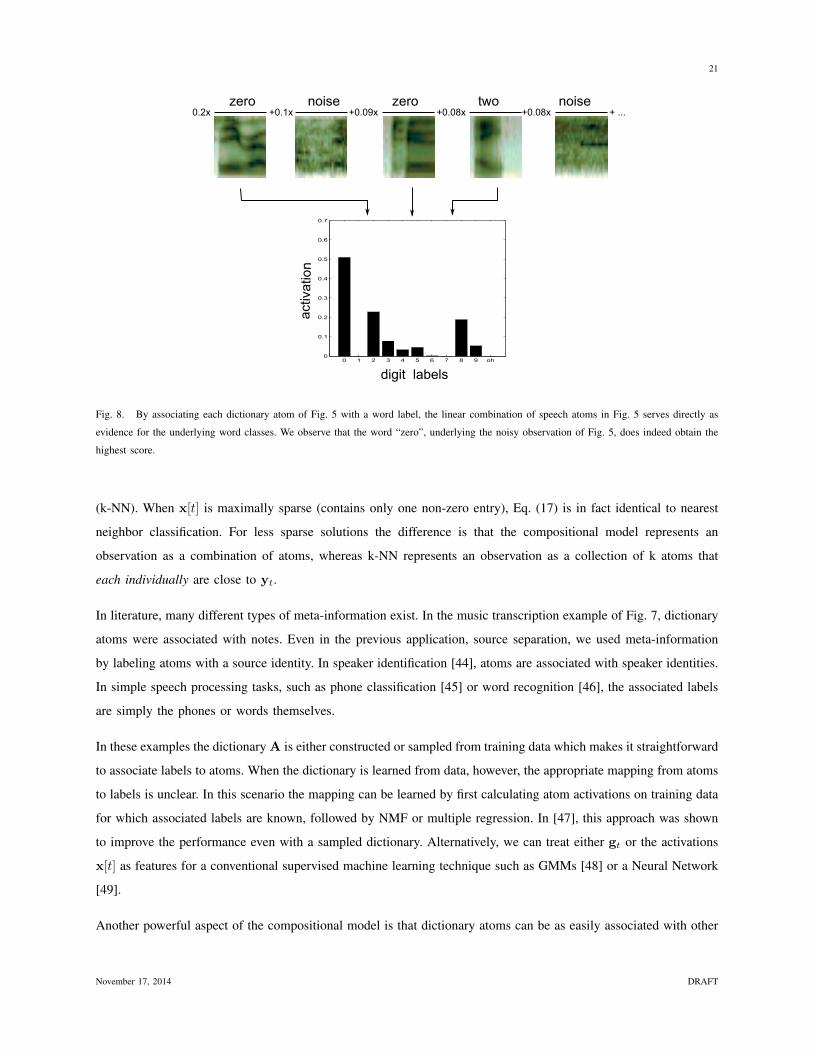
vector g are an unscaled score proportional to the presence of class labels in the observation. An example of

this procedure is given in Fig. 8, where the dictionary atoms of the source separation example of Fig. 5 are now

associated with word labels.

The formulation in Eq. (17) is closely related to several other techniques such as k nearest neighbor classification


21

0 1 2 3 4 5 6 7 8 9 oh0

0.1

0.2

0.3

0.4

0.5

0.6

0.7

zero noise zero two noise 0.2x +0.1x +0.09x +0.08x +0.08x + ...

digit labels

activ

atio

n

Fig. 8. By associating each dictionary atom of Fig. 5 with a word label, the linear combination of speech atoms in Fig. 5 serves directly as

evidence for the underlying word classes. We observe that the word “zero”, underlying the noisy observation of Fig. 5, does indeed obtain the

highest score.

(k-NN). When x[t] is maximally sparse (contains only one non-zero entry), Eq. (17) is in fact identical to nearest

neighbor classification. For less sparse solutions the difference is that the compositional model represents an

observation as a combination of atoms, whereas k-NN represents an observation as a collection of k atoms that

each individually are close to yt.

In literature, many different types of meta-information exist. In the music transcription example of Fig. 7, dictionary

atoms were associated with notes. Even in the previous application, source separation, we used meta-information

by labeling atoms with a source identity. In speaker identification [44], atoms are associated with speaker identities.

In simple speech processing tasks, such as phone classification [45] or word recognition [46], the associated labels

are simply the phones or words themselves.

In these examples the dictionary A is either constructed or sampled from training data which makes it straightforward

to associate labels to atoms. When the dictionary is learned from data, however, the appropriate mapping from atoms

to labels is unclear. In this scenario the mapping can be learned by first calculating atom activations on training data

for which associated labels are known, followed by NMF or multiple regression. In [47], this approach was shown

to improve the performance even with a sampled dictionary. Alternatively, we can treat either gt or the activations

x[t] as features for a conventional supervised machine learning technique such as GMMs [48] or a Neural Network

[49].

Another powerful aspect of the compositional model is that dictionary atoms can be as easily associated with other


22

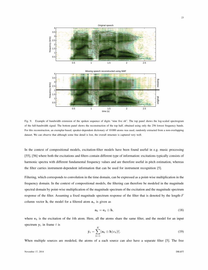
kinds of information, for example audio. Consider for example a bandwidth extension task [9], [50], where the

goal is to estimate a full-spectrum audio signal given a bandwidth-limited audio signal. This is a useful operation

to perform since in many audio transmission cases high frequency information is removed to reduce the amount

of information to transmit, something that negatively impacts intelligibility and the perception of quality. In order

to use the compositional model approach for this task, two dictionaries are first constructed: a bandwidth-limited

dictionary A and a full-bandwidth dictionary L. The atoms in the dictionaries should be coupled, i.e., each atom

in A should represent a band-limited version of the corresponding atom in L. This can be done through training

on parallel corpora of full-bandwidth and band-limited signals, or by calculating L from A, if the details of the

band-limitation process are known and can be modeled computationally. We then estimate the atom activations x[t]

using the limited-bandwidth observation yt and the limited-bandwidth dictionary A. Finally, direct application of

Eq. (17) serves as a replacement for the audio reconstruction Ax[t] and yields a full-bandwidth reconstruction. We

illustrate this process in Fig. 9. Very similar principles underlay voice conversion, in which the associated audio is

another speaker [51], [52].

Missing data imputation [53], [54], [29] is closely related to bandwidth extension in that the goal is to estimate a

full-spectrum audio signal, but with the difference that the missing data is not a set of predetermined frequency

bands but rather arbitrary located time-frequency entries of the spectrogram. Algorithms for compositional models

can be easily modified so that model parameters are estimated using only a part of the observed data (ignoring

missing data) [54], [29], but the model output can be calculated also for entries corresponding to the missing data.

Provided that there is a sufficient amount of observed (not missing) data which will allow estimating the activations

(and atoms in the case of unsupervised processing), reasonable estimates of missing values can be obtained because

of dependencies between observed and missing values. In general the quality of a model can be judged by its

ability to make predictions, and the capability of compositional models to predict missing data also illustrates its

effectiveness.

EXCITATION-FILTER MODEL AND CHANNEL COMPENSATION

Creating dictionaries from training data as presented earlier in the paper yields accurate representations, as long as

the data from which the dictionaries are learned match with the observed data. In many practical situations this is

not the case, and there is a need to adapt the learned dictionaries. Moreover, often we have knowledge about the

types of sources to be modeled, for example that they are musical instruments, but do not have suitable training

data to estimate the dictionaries in an supervised manner.

Natural sound sources can be modeled as an excitation signal being filtered by an instrument body filter or vocal

tract filter. This kind of excitation-filter or source-filter models have been very effective for example in speech

coding (several codecs use it). In addition to modeling the properties of a body filter, the filter can also model the

response from a source to a microphone, and therefore to do channel compensation as well.


23

Original speech

freq

uenc

y (k

Hz)

0.5 1 1.5 2 2.5

0.5

1

1.5

2

2.5

3

3.5

4

Missing speech reconstructed using NMF

time (s)

freq

uenc

y (k

Hz)

mis

sing

orig

inal

0.5 1 1.5 2 2.5

0.5

1

1.5

2

2.5

3

3.5

4

Fig. 9. Example of bandwidth extension of the spoken sequence of digits “nine five oh”. The top panel shows the log-scaled spectrogram

of the full-bandwidth signal. The bottom panel shows the reconstruction of the top half, obtained using only the 256 lowest frequency bands.

For this reconstruction, an exemplar-based, speaker-dependent dictionary of 10 000 atoms was used, randomly extracted from a non-overlapping

dataset. We can observe that although some fine detail is lost, the overall structure is captured very well.

In the context of compositional models, excitation-filter models have been found useful in e.g. music processing

[55], [56] where both the excitations and filters contain different type of information: excitations typically consists of

harmonic spectra with different fundamental frequency values and are therefore useful in pitch estimation, whereas

the filter carries instrument-dependent information that can be used for instrument recognition [5].

Filtering, which corresponds to convolution in the time domain, can be expressed as a point-wise multiplication in the

frequency domain. In the context of compositional models, the filtering can therefore be modeled in the magnitude

spectral domain by point-wise multiplication of the magnitude spectrum of the excitation and the magnitude spectrum

response of the filter. Assuming a fixed magnitude spectrum response of the filter that is denoted by the length-F

column vector h, the model for a filtered atom an is given as

ak = ek ⊗ h, (18)

where ek is the excitation of the kth atom. Here, all the atoms share the same filter, and the model for an input

spectrum yt in frame t is

yt =

K∑k=1

(ak ⊗ h)xk[t]. (19)

When multiple sources are modeled, the atoms of a each source can also have a separate filter [5]. The free


24

parameters of an excitation-filter model can be estimated using the principles described in the previous sections

— by applying iteratively update rules for each of the terms that decrease the divergence between an observed

spectrogram and the model. Even for complex models like this, deriving update rules is rather straightforward using

the principles presented in [57], [58], [3].

Excitations can often be parameterized quite compactly: for example in music signal processing, it is known that

many sources are harmonic, and many sources have a distinct set of fundamental frequency values that they can

produce, each corresponding to a harmonic spectrum with different fundamental f0. Therefore, many excitation-filter

models use a fixed set of harmonic excitations [5], [55], [58].

The filters, on the other hand, are specific to each instrument, recording environment or microphone. In order

to avoid that filters model harmonic structures when learned unsupervised, smooth filters over frequency can be

obtained for example by using constraints on two adjacent filter values [56], or by modeling filters a sum of smooth

elementary filter atoms [55].

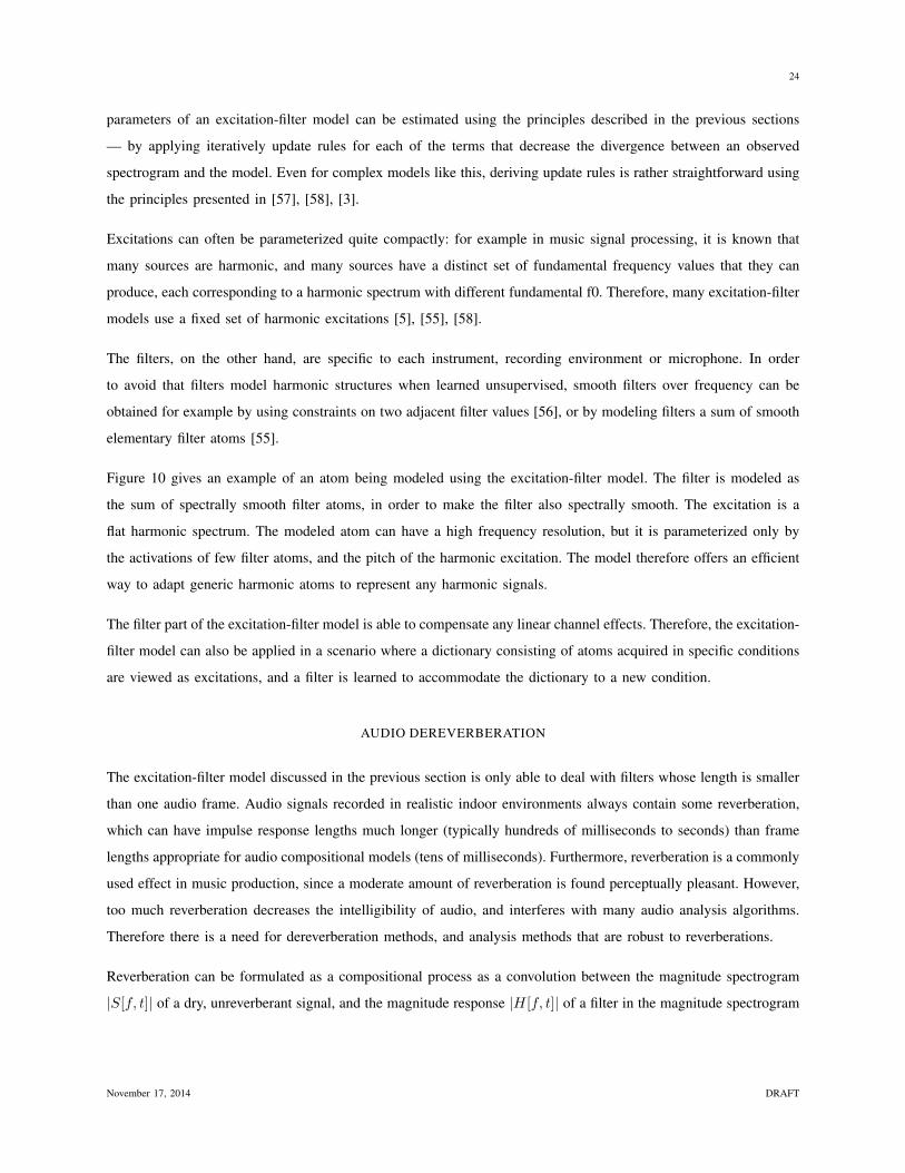
Figure 10 gives an example of an atom being modeled using the excitation-filter model. The filter is modeled as

the sum of spectrally smooth filter atoms, in order to make the filter also spectrally smooth. The excitation is a

flat harmonic spectrum. The modeled atom can have a high frequency resolution, but it is parameterized only by

the activations of few filter atoms, and the pitch of the harmonic excitation. The model therefore offers an efficient

way to adapt generic harmonic atoms to represent any harmonic signals.

The filter part of the excitation-filter model is able to compensate any linear channel effects. Therefore, the excitation-

filter model can also be applied in a scenario where a dictionary consisting of atoms acquired in specific conditions

are viewed as excitations, and a filter is learned to accommodate the dictionary to a new condition.

AUDIO DEREVERBERATION

The excitation-filter model discussed in the previous section is only able to deal with filters whose length is smaller

than one audio frame. Audio signals recorded in realistic indoor environments always contain some reverberation,

which can have impulse response lengths much longer (typically hundreds of milliseconds to seconds) than frame

lengths appropriate for audio compositional models (tens of milliseconds). Furthermore, reverberation is a commonly

used effect in music production, since a moderate amount of reverberation is found perceptually pleasant. However,

too much reverberation decreases the intelligibility of audio, and interferes with many audio analysis algorithms.

Therefore there is a need for dereverberation methods, and analysis methods that are robust to reverberations.

Reverberation can be formulated as a compositional process as a convolution between the magnitude spectrogram

|S[f, t]| of a dry, unreverberant signal, and the magnitude response |H[f, t]| of a filter in the magnitude spectrogram


25

elementary filter atoms activations of filter atoms

weighted filter atoms

learned filter

synthetic harmonic excitation

modeled atom

⊗

⊗

Σ

Fig. 10. Modeling atoms with the excitation-filter model. The filter is modeled as the sum of elementary filter atoms (upper left), weighted by

activations (upper right). The filter is point-wise multiplied by a synthetic harmonic excitation (right) to get an atom (bottom).

domain [59], [60]:

|Y [f, t]| ≈M∑τ=0

|S[f, t− τ ]||H[f, τ ]| (20)

≡ |S[f, t]| ∗ |H[f, t]|, (21)

where M is the length of the filter (in frames). Blind estimation of dry signals and reverberation filters is not

feasible since the model is ambiguous, and the roles of the source and the impulse response can end up swapped if

other restrictions are not used. A suitable a priori information to regularize the model can be e.g. sparseness [60],

or dictionary-based model [59]. Thus in practice, we can model |S(f, t)| using another compositional model. The

model parameters can be estimated using the principles explained above, i.e., by minimizing a divergence between

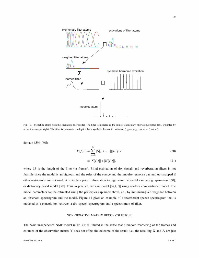
an observed spectrogram and the model. Figure 11 gives an example of a reverberant speech spectrogram that is

modeled as a convolution between a dry speech spectrogram and a spectrogram of filter.

NON-NEGATIVE MATRIX DECONVOLUTIONS

The basic unsupervised NMF model in Eq. (1) is limited in the sense that a random reordering of the frames and

columns of the observation matrix Y does not affect the outcome of the result, i.e., the resulting X and A are just


26

time (s)

fre

qu

en

cy (

Hz)

reverberant spectrogram |Y[f,t]|

0 0.5 1 1.5 2 2.50

1000

2000

3000

4000

5000

time (s)

dry spectrogram |S[f,t]|

0 0.5 1 1.5 2 2.5

time (s)

reverberation filter |H[f,t]|

0 0.5 1

≈ ∗

Fig. 11. The magnitude spectrogram of a reverberant signal (left panel) can be approximated as the convolution between the spectrograms of

a dry signal (middle panel) and the impulse response of the reverberation.

reordered versions of X and A that would have been obtained without reordering of Y.

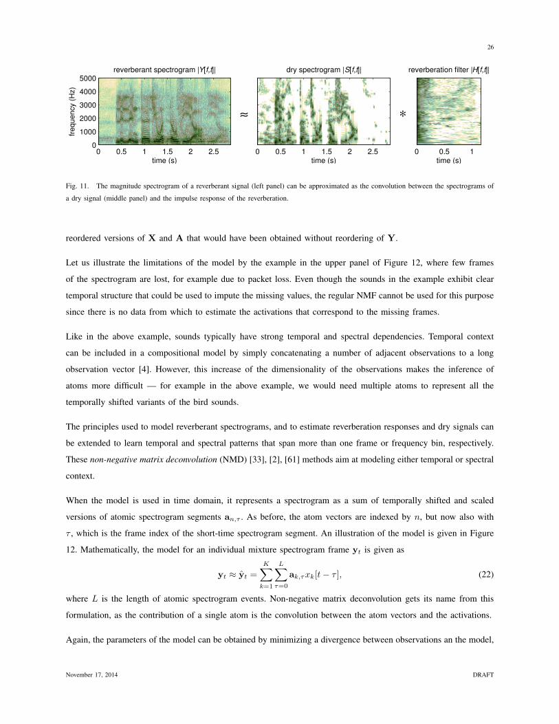
Let us illustrate the limitations of the model by the example in the upper panel of Figure 12, where few frames

of the spectrogram are lost, for example due to packet loss. Even though the sounds in the example exhibit clear

temporal structure that could be used to impute the missing values, the regular NMF cannot be used for this purpose

since there is no data from which to estimate the activations that correspond to the missing frames.

Like in the above example, sounds typically have strong temporal and spectral dependencies. Temporal context

can be included in a compositional model by simply concatenating a number of adjacent observations to a long

observation vector [4]. However, this increase of the dimensionality of the observations makes the inference of

atoms more difficult — for example in the above example, we would need multiple atoms to represent all the

temporally shifted variants of the bird sounds.

The principles used to model reverberant spectrograms, and to estimate reverberation responses and dry signals can

be extended to learn temporal and spectral patterns that span more than one frame or frequency bin, respectively.

These non-negative matrix deconvolution (NMD) [33], [2], [61] methods aim at modeling either temporal or spectral

context.

When the model is used in time domain, it represents a spectrogram as a sum of temporally shifted and scaled

versions of atomic spectrogram segments an,τ . As before, the atom vectors are indexed by n, but now also with

τ , which is the frame index of the short-time spectrogram segment. An illustration of the model is given in Figure

12. Mathematically, the model for an individual mixture spectrogram frame yt is given as

yt ≈ yt =

K∑k=1

L∑τ=0

ak,τxk[t− τ ], (22)

where L is the length of atomic spectrogram events. Non-negative matrix deconvolution gets its name from this

formulation, as the contribution of a single atom is the convolution between the atom vectors and the activations.

Again, the parameters of the model can be obtained by minimizing a divergence between observations an the model,


27

freq

uenc

y (k

Hz)

spectrogram matrix Y with missing frames

0.5 1 1.5 2 2.5 3 3.5 4 4.50

1

2

3

4

5

component a1,τ

freq

uenc

y (k

Hz)

τ0

1

2

3

4

component a2,τ

τ 0 1 2 3 4 50

0.2

0.4

0.6

0.8

1

time (s)

ampl

itude

activations X

Fig. 12. Illustration of the non-negative matrix deconvolution model. The top panel represents the magnitude spectrogram of a signal consisting

of three bird sounds (Friedmann’s Lark) and background noises. The spectrogram is modeled using non-negative matrix deconvolution (NMD) to

decompose the signal into bird sounds (component 1) and background noises (component 2). The compositional model represents the spectrogram

as the weighted and delayed sum of two short event spectrogram segments (left panels). The curves on the bottom panel show the weights for

each delay. The impulses in the curves correspond to start times of bird sound events in the mixture. The events have been correctly found

event though some of the frames in the mixture signal are missing (black vertical bar). Since NMD models the mixture as a sum of segments

longer than the missing-frame segment, the model parameters can be used to predict the missing frames.

while constraining the model parameters to non-negative values. In an unsupervised scenario where both the atom

vectors and their activations are estimated, care must be taken to limit the number of atoms and the length of events,

in order to avoid overfitting.

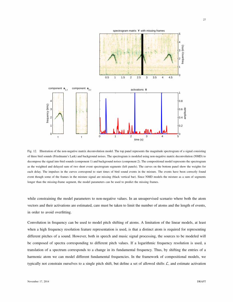
Convolution in frequency can be used to model pitch shifting of atoms. A limitation of the linear models, at least

when a high frequency resolution feature representation is used, is that a distinct atom is required for representing

different pitches of a sound. However, both in speech and music signal processing, the sources to be modeled will

be composed of spectra corresponding to different pitch values. If a logarithmic frequency resolution is used, a

translation of a spectrum corresponds to a change in its fundamental frequency. Thus, by shifting the entries of a

harmonic atom we can model different fundamental frequencies. In the framework of compositional models, we

typically not constrain ourselves to a single pitch shift, but define a set of allowed shifts L, and estimate activation


28

time (seconds)

freq

uenc

y sh

ift τ

activations x1,τ [t]

0 1 2 3 4

100

200

300

400

500

0 10 200

500

1000

1500

2000

log−

freq

uenc

y in

dex

f

amplitude

atom a1

log−

freq

uenc

y in

dex

f

observed spectrogram Y

200

400

600

800

1000

1200

1400

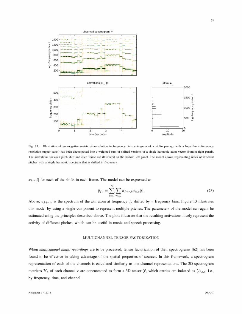
Fig. 13. Illustration of non-negative matrix deconvolution in frequency. A spectrogram of a violin passage with a logarithmic frequency

resolution (upper panel) has been decomposed into a weighted sum of shifted versions of a single harmonic atom vector (bottom right panel).

The activations for each pitch shift and each frame are illustrated on the bottom left panel. The model allows representing notes of different

pitches with a single harmonic spectrum that is shifted in frequency.

xk,τ [t] for each of the shifts in each frame. The model can be expressed as

yf,t =

K∑k=1

∑τ∈L

af+τ,kxk,τ [t]. (23)

Above, af+τ,k is the spectrum of the kth atom at frequency f , shifted by τ frequency bins. Figure 13 illustrates

this model by using a single component to represent multiple pitches. The parameters of the model can again be

estimated using the principles described above. The plots illustrate that the resulting activations nicely represent the

activity of different pitches, which can be useful in music and speech processing.

MULTICHANNEL TENSOR FACTORIZATION

When multichannel audio recordings are to be processed, tensor factorization of their spectrograms [62] has been

found to be effective in taking advantage of the spatial properties of sources. In this framework, a spectrogram

representation of each of the channels is calculated similarly to one-channel representations. The 2D-spectrogram

matrices Yc of each channel c are concatenated to form a 3D-tensor Y , which entries are indexed as Yf,t,c, i.e.,

by frequency, time, and channel.


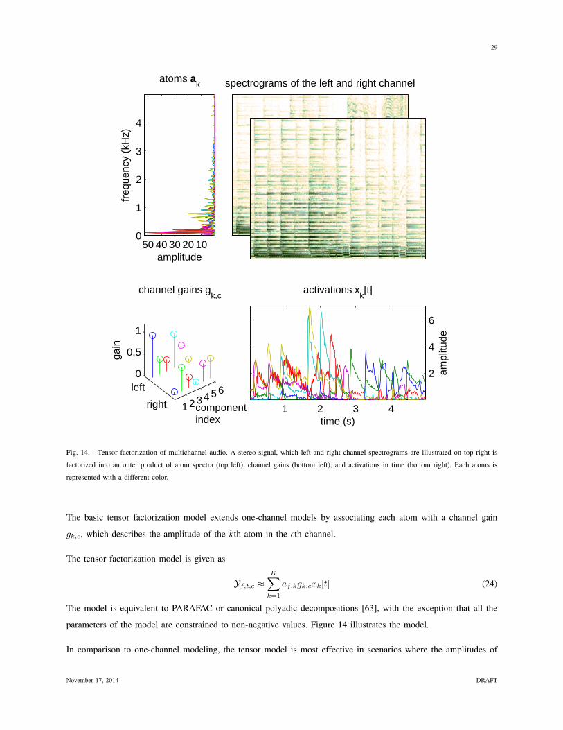
29

spectrograms of the left and right channel

1 2 3 4

2

4

6

time (s)

ampl

itude

activations xk[t]

10203040500

1

2

3

4fr

eque

ncy

(kH

z)

amplitude

atoms ak

1 2 3 4 5 6right

left0

0.5

1

componentindex

channel gains gk,c

gain

Fig. 14. Tensor factorization of multichannel audio. A stereo signal, which left and right channel spectrograms are illustrated on top right is

factorized into an outer product of atom spectra (top left), channel gains (bottom left), and activations in time (bottom right). Each atoms is

represented with a different color.

The basic tensor factorization model extends one-channel models by associating each atom with a channel gain

gk,c, which describes the amplitude of the kth atom in the cth channel.

The tensor factorization model is given as

Yf,t,c ≈K∑k=1

af,kgk,cxk[t] (24)

The model is equivalent to PARAFAC or canonical polyadic decompositions [63], with the exception that all the

parameters of the model are constrained to non-negative values. Figure 14 illustrates the model.

In comparison to one-channel modeling, the tensor model is most effective in scenarios where the amplitudes of


30

individual sources are different in each channel. The level differences depend on the way the signals are produced.

For example in commercially produced music, especially in music produced between the 60s and the 80s, stereo

panning was often used as a strong effect, and sources may have significantly different amplitudes. Similarly, if a

signal is captured by multiple microphones that are far away from each other, source-wise amplitude differences

between microphones are large. When a signal is captured by a microphone array where the microphones are close

to each other, the amplitude differences between channels are typically small, but there are clear phase differences

between the signals. In this scenario, techniques [10], [64] that model spectrogram magnitudes with the basic NMF

model and phase differences between the channels with another model have shown potential.

DISCUSSION

Even though compositional models are a fairly new technique in the context of audio signal processing, as we have

shown in this article they are applicable to many fundamental audio processing tasks such as source separation,

classification, and dereverberation. The compositional nature of the model, the modeling of a spectrogram as a non-

negative sum of atoms having a fixed spectrum and a time-varying gain, is intuitive and offers clear interpretations of

the model parameters. This makes it easy to analyze representations obtained with the model, both algorithmically

and manually, for example by visualizing the models.

The linear nature of the model also offers other advantages. Even when more complex models are used that combine

multiple extensions described earlier, the linearity makes it straightforward to derive optimization algorithms for the

estimation of the model parameters. Unlike some methods conventionally used for modeling multiple co-occurring

sources (e.g. factorial hidden Markov models), the computational complexity of compositional model algorithms

scales linearly as the function of the number of sources.

Compositional models have also some limitations. In the context of audio processing they are mainly applied on

magnitudes of time-frequency representations, and require additional phase information for signal reconstruction.

Therefore the models have mainly applications in analyzing or processing existing signals, and their applicability in

e.g. sound synthesis is limited. Because of the linearity of the models, compositional models also do not suit well for

modeling non-linear phenomena. Compositional models use iterative algorithms for finding the model parameters,

and their computational complexity is quite significant when large dictionaries are used. Thus, the accuracy of the

models may need to be compromised in the case of real-time implementations. The optimization problems involved

with compositional models are often non-convex, and therefore different algorithms and their initializations lead

to different solutions, which needs to be taken into account when results obtained with the models are examined.

Even though designing algorithms for new compositional models is in general rather straightforward, the sensitivity

of the algorithms to get stuck into a local minimum far away from the global optimum increases as the structure

of the model becomes more complex, and the model order increases. In order to get more accurate solutions with

complex models, carefully designed initializations or regularizations may be needed.


31

Compositional models provide a single framework that enables modeling of several phenomena present in real

world-audio: additive sources, sources consisting of multiple sound objects, convolutive noise, and reverberation.

Frameworks that combine these in a systematic and flexible way have already been presented [58], [57]. Moreover,

the ability of the models to couple acoustic and other types of information enables audio analysis and recognition

directly using the model. To be able to handle all of this within a single framework is a great advantage in comparison

to methods that tackle just a specific task, since it offers the potential of jointly modeling multiple effects that affect

each other, such as reverberation and source mixing.

ACKNOWLEDGMENTS

Tuomas Virtanen has been financially supported by Academy of Finland, grant number 258708. The research of

Jort F. Gemmeke was funded by the IWT-SBO project ALADIN contract 100049.

AUTHORS

Tuomas Virtanen ([email protected]) is an Academy Research Fellow and an adjunct professor in Department

of Signal Processing, Tampere University of Technology (TUT), Finland. He received the M.Sc. and Doctor of

Science degrees in information technology from TUT in 2001 and 2006, respectively. He has also been working

as a research associate at Cambridge University Engineering Department, UK. He is known for his pioneering

work on single-channel sound source separation using non-negative matrix factorization based techniques, and their

application to noise-robust speech recognition, music content analysis and audio classification. In addition to the

above topics, his research interests include content analysis of audio signals and machine learning.

Jort Florent Gemmeke ([email protected]) is a postdoctoral researcher at the KU Leuven, Belgium. He

received the M.Sc degree in physics from the Universiteit van Amsterdam (UvA) in 2005. In 2011, he received the

Ph.D degree from the University of Nijmegen on the subject of noise robust ASR using missing data techniques. He

is known for pioneering the field of exemplar-based noise robust ASR. His research interests are automatic speech

recognition, source separation, noise robustness and acoustic modeling, in particular exemplar-based methods and

methods using sparse representations.

Bhiksha Raj ([email protected]) is an associate professor in the Language Technologies Institute of Carnegie

Mellon University, with additional affiliations to the Machine Learning and Electrical and Computer Engineering

departments of the University. Dr Raj completed his PhD from Carnegie Mellon University in 2000. From 2001-2008

he worked at Mitsubishi Electric Research Labs in Cambridge MA, where he led the research effort on speech

processing. He has been at CMU since 2008. Dr Raj’s research interests include speech and audio processing,

automatic speech recognition, natural language processing and machine learning.


32

Paris Smaragdis ([email protected]) is an Assistant Professor in the departments of Computer Science and Electrical

Engineering at the University of Illinois in Urbana Champaign and a research scientist at Adobe. He received his

Ph.D from MIT in 2003, and was at Adobe research prior to joining UIUC. He is the inventor of frequency-domain

independent component analysis and several of the approaches that are now common in compositional-model based

signal enhancement. His interest lie in computer audition, machine learning and speech recognition.

REFERENCES

[1] A. Cichocki, R. Zdunek, A. H. Phan, and S. Amari, Nonnegative Matrix and Tensor Factorizations: Applications to Exploratory Multi-way

Data Analysis and Blind Source Separation. Wiley, 2009.

[2] P. Smaragdis, “Convolutive speech bases and their application to supervised speech separation,” IEEE Transactions on Audio, Speech, and

Language Processing, vol. 15, no. 1, pp. 1 – 12, 2007.

[3] T. Virtanen, “Monaural sound source separation by non-negative matrix factorization with temporal continuity and sparseness criteria,”

IEEE Transactions on Audio, Speech, and Language Processing, vol. 15, no. 3, pp. 1066 – 1074, 2007.

[4] J. Gemmeke, T. Virtanen, and A. Hurmalainen, “Exemplar-based sparse representations for noise robust automatic speech recognition,”


[5] T. Heittola, A. Klapuri, and T. Virtanen, “Musical instrument recognition in polyphonic audio using source-filter model for sound separation,”

in Proceedings of International Conference on Music Information Retrieval, Kobe, Japan, 2009.

[6] J. T. Geiger, F. Weninger, A. Hurmalainen, J. F. Gemmeke, M. Wllmer, B. Schuller, G. Rigoll, and T. Virtanen, “The TUM+TUT+KUL

approach to the CHiME Challenge 2013: Multi-stream ASR exploiting BLSTM networks and sparse NMF,” in Proceedings of The 2nd

International Workshop on Machine Listening in Multisource Environments, Vancouver, Canada, 2013.

[7] Y.-C. Cho and S. Choi, “Nonnegative features of spectro-temporal sounds for classification,” Pattern Recognition Letters, vol. 26, no. 9,

pp. 1327 – 1336, 2005.

[8] N. Bertin, R. Badeau, and E. Vincent, “Enforcing harmonicity and smoothness in Bayesian non-negative matrix factorization applied to

polyphonic music transcription,” IEEE Transactions on Audio, Speech, and Language Processing, vol. 18, no. 3, pp. 538 – 549, 2010.

[9] D. Bansal, B. Raj, and P. Smaragdis, “Bandwidth expansion of narrowband speech using non-negative matrix factorization,” in 9th European

Conference on Speech Communication and Technology, Lisbon, Portugal, 2003.

[10] A. Ozerov and C. Fevotte, “Multichannel nonnegative matrix factorization in convolutive mixtures for audio source separation,” IEEE

Transactions on Audio, Speech, and Language Processing, vol. 18, no. 3, pp. 550 – 563, 2010.

[11] M. D. Plumbley, T. Blumensath, L. Daudet, R. Gribonval, and M. E. Davies, “Sparse representations in audio & music: from coding to

source separation,” Proceedings of the IEEE, vol. 98, no. 6, pp. 995–1005, 2009.

[12] J. Nikunen and T. Virtanen, “Object-based audio coding using non-negative matrix factorization for the spectrogram representation,” in

Proceedings of the 128th Audio Engineering Society Convention, London, UK, 2010.

[13] C. Fevotte, N. Bertin, and J.-L. Durrieu, “Nonnegative matrix factorization with the Itakura-Saito divergence. With application to music

analysis,” Neural Computation, vol. 21, no. 3, pp. 793–830, 2009.


33

[14] M. Shashanka, B. Raj, and P. Smaragdis, “Sparse overcomplete latent variable decomposition of counts data,” in Proceedings of Neural

Information Processing Systems, Vancouver, Canada, 2007.

[15] C. Ding, T. Li, and W. Ping, “On the equivalence between non-negative matrix factorization and probabilistic latent semantic indexing,”

Computational Statistics & Data Analysis, vol. 52, no. 8, pp. 3913 – 3927, 2008.

[16] E. Zwicker and H. Fastl, Psychoacoustics: Facts and Models. Springer-Verlag, 1990.

[17] B. C. J. Moore, Ed., Hearing—Handbook of Perception and Cognition, 2nd ed. San Diego, California: Academic Press, 1995.

[18] B. King, C. Fevotte, and P. Smaragdis, “Optimal cost function and magnitude power for NMF-based speech separation and music

interpolation,” in Proceedings of IEEE International Workshop on Machine Learning for Signal Processing, Santander, Spain, 2012.

[19] J. Carabias-Orti, F. Rodriguez-Serrano, P. Vera-Candeas, F. Canadas-Quesada, and N. Ruiz-Reyes, “Constrained non-negative sparse coding

using learnt instrument templates for realtime music transcription,” Engineering Applications of Artificial Intelligence, pp. 1671 – 1680,

2013.

[20] F. Weninger and B. Schuller, “Optimization and parallelization of monaural source separation algorithms in the openBliSSART toolkit,”

Journal of Signal Processing Systems, vol. 69, no. 3, pp. 267 – 277, 2012.

[21] C. Fevotte and J. Idier, “Algorithms for nonnegative matrix factorization with the beta-divergence,” Neural Computation, vol. 23, pp.

2421–2456, 2011.

[22] D. D. Lee and H. S. Seung, “Algorithms for non-negative matrix factorization,” in Proceedings of Neural Information Processing Systems,

Denver, USA, 2000, pp. 556–562.

[23] R. Zdunek and A. Cichocki, “Nonnegative matrix factorization with constrained second-order optimization,” Signal Processing, vol. 87,

no. 8, pp. 1904 – 1916, 2007.

[24] J. Kim and H. Park, “Fast nonnegative matrix factorization: An active-set-like method and comparisons,” SIAM Journal on Scientific

Computing, vol. 33, no. 6, pp. 3261 – 3281, 2011.

[25] T. Virtanen, J. Gemmeke, and B. Raj, “Active-set Newton algorithm for overcomplete non-negative representations of audio,” IEEE

Transactions on Audio, Speech, and Language Processing, 2013, accepted for publication.

[26] T. Hofmann, “Unsupervised learning by probabilistic latent semantic analysis,” Machine Learning, vol. 42, no. 1-2, pp. 177 – 196, 2001.

[27] M. Shashanka, B. Raj, and P. Smaragdis, “Probabilistic latent variable models as non-negative factorizations,” Computational Intelligence

and Neuroscience, vol. 2008, 2008.

[28] G. J. Mysore, P. Smaragdis, and B. Raj, “Non-negative hidden Markov modeling of audio with application to source separation,” in

Proceedings of the 9th International Conference on Latent Variable Analysis and Signal Separation, St. Malo, France, 2010.

[29] P. Smaragdis, B. Raj, and M. Shashanka, “Missing data imputation for time-frequency representations of audio signals,” Journal of Signal

Processing Systems, vol. 11, no. 3, pp. 361 – 370, 2011.

[30] H. Laurberg, M. G. Christensen, M. D. Plumbley, L. K. Hansen, and S. H. Jensen, “Theorems on positive data: On the uniqueness of

NMF,” Computational Intelligence and Neuroscience, vol. 2008, 2008.

[31] J. Eggert and E. Korner, “Sparse coding and NMF,” in IEEE International Joint Conference on Neural Networks, Budapest, Hungary,

2004, pp. 2529–2533.


34

[32] P. O. Hoyer, “Non-negative matrix factorization with sparseness constraints,” Journal of Machine Learning Research, vol. 5, pp. 1457–1469,

2004.

[33] P. D. O. Grady, “Sparse separation of underdetermined speech mixtures,” Ph.D. dissertation, National University of Ireland, Maynooth,

2007.

[34] T. Virtanen, “Spectral covariance in prior distributions of non-negative matrix factorization based speech separation,” in Proceedings of

European Signal Processing Conference, Glasgow, Scotland, 2009.

[35] P. Smaragdis, M. Shashanka, and B. Raj, “A sparse non-parametric approach for single channel separation of known sounds,” in Proceedings

of Neural Information Processing Systems, Vancouver, Canada, 2009.

[36] D. Griffin and J. Lim, “Signal estimation from modified short-time Fourier transform,” IEEE Transactions on Acoustics, Speech, and Signal

Processing, vol. 32, pp. 236–242, 1984.

[37] J. Le Roux and E. Vincent, “Consistent Wiener filtering for audio source separation,” IEEE Signal Processing Letters, vol. 20, no. 3, pp.

217 – 220, 2013.

[38] M. Aharon, M. Elad, and A. Bruckstein, “K-SVD and its non-negative variant for dictionary design,” in Proceedings of SPIE Conference

on Wavelet Applications in Signal and Image Processing XI, San Diego, USA, 2005.

[39] R. G. Baraniuk, “Compressive sensing,” IEEE Signal Processing Magazine, vol. 24, no. 4, pp. 118–121, 2007.

[40] A. Lefevre, F. Bach, and C. Fevotte, “Itakura-Saito nonnegative matrix factorization with group sparsity,” in Proceedings of IEEE

International Conference on Audio, Speech and Signal Processing, Prague, Czech Republic, 2011.

[41] A. T. Cemgil, “Bayesian inference for nonnegative matrix factorisation models,” Computational Intelligence and Neuroscience, vol. 2009,

2009.

[42] M. N. Schmidt and M. Mørup, “Infinite non-negative matrix factorizations,” in Proceedings of European Signal Processing Conference,

Aalborg, Denmark, 2010.

[43] M. N. Schmidt, O. Winther, and L. K. Hansen, “Bayesian non-negative matrix factorization,” in Proceedings of the 8th International

Conference on Independent Component Analysis and Blind Signal Separation, Paraty, Brazil, 2009.

[44] A. Hurmalainen, R. Saeidi, and T. Virtanen, “Group sparsity for speaker identity discrimination in factorisation-based speech recognition,”

in Proceedings of Interspeech 2012, Portland, USA, 2012.

[45] T. N. Sainath, A. Carmi, D. Kanevsky, and B. Ramabhadran, “Bayesian compressive sensing for phonetic classification,” in Proceedings

of IEEE International Conference on Audio, Speech and Signal Processing, Dallas, USA, 2010.

[46] J. Gemmeke, L. ten Bosch, L. Boves, and B. Cranen, “Using sparse representations for exemplar based continuous digit recognition,” in

Proceedings of European Signal Processing Conference, Glasgow, Scotland, 2009.

[47] K. Mahkonen, A. Hurmalainen, T. Virtanen, and J. F. Gemmeke, “Mapping sparse representation to state likelihoods in noise-robust

automatic speech recognition,” in Proceedings of Interspeech 2011, Florence, Italy, 2011, pp. 465–468.

[48] Y. Sun, B. Cranen, J. F. Gemmeke, L. Boves, L. ten Bosch, and M. M. Doss, “Using sparse classification outputs as feature observations

for noise-robust ASR,” in Proceedings of Interspeech 2012, Portland, USA, 2012.

[49] T. N. Sainath, D. Nahamoo, D. Kanevsky, and B. Ramabhadran, “Enhancing exemplar-based posteriors for speech recognition tasks,” in

Proceedings of Interspeech 2012, Portland, USA, 2012.


35

[50] B. Raj, R. Singh, M. Shashanka, and P. Smaragdis, “Bandwidth expansion with a Polya Urn model,” in Proceedings of IEEE International

Conference on Audio, Speech and Signal Processing, Honolulu, USA, 2007.

[51] R. Takashima, T. Takiguchi, and Y. Ariki, “Exemplar-based voice conversion in noisy environment,” in Proceedings of IEEE Spoken

Language Technology Workshop, 2012, pp. 313–317.

[52] Z. Wu, T. Virtanen, T. Kinnunen, E. S. Chng, and H. Li, “Exemplar-based voice conversion using non-negative spectrogram deconvolution,”

in Proceedings of 8th ISCA Speech Synthesis Workshop, Barcelona, Spain, 2013.

[53] J. F. Gemmeke, H. Van hamme, B. Cranen, and L. Boves, “Compressive sensing for missing data imputation in noise robust speech

recognition,” IEEE Journal of Selected Topics in Signal Processing, vol. 4, no. 2, pp. 272–287, 2010.

[54] J. Le Roux, H. Kameoka, N. Ono, A. de Cheveigne, and S. Sagayama, “Computational auditory induction as a missing-data model-fitting

problem with Bregman divergence,” SIAM Journal on Scientific Computing, vol. 54, no. 5, pp. 658 – 676, 2011.

[55] J.-L. Durrieu, B. David, and G. Richard, “A musically motivated mid-level representation for pitch estimation and musical audio source

separation,” IEEE Journal of Selected Topics in Signal Processing, vol. 5, no. 6, pp. 1180 – 1191, 2011.

[56] J. Carabias-Orti, T. Virtanen, P. Vera-Candeas, N. Ruiz-Reyes, and F. Canadas-Quesada, “Musical instrument sound multi-excitation model

for non-negative spectrogram factorization,” IEEE Journal of Selected Topics in Signal Processing, vol. 5, no. 6, pp. 1144 – 1158, 2011.

[57] Y. K. Yilmaz, A. T. Cemgil, and U. Simsekli, “Generalized coupled tensor factorization,” in Proceedings of Neural Information Processing

Systems, Granada, Spain., 2011.

[58] A. Ozerov, E. Vincent, and F. Bimbot, “A general flexible framework for the handling of prior information in audio source separation,”


[59] N. Yasuraoka, H. Kameoka, T. Yoshioka, and H. G. Okuno, “I-divergence-based dereverberation method with auxiliary function approach,”

in Proceedings of IEEE International Conference on Audio, Speech and Signal Processing, Prague, Czech Republic, 2011.

[60] R. Singh, B. Raj, and P. Smaragdis, “Latent-variable decomposition based dereverberation of monaural and multi-channel signals,” in

Proceedings of IEEE International Conference on Audio, Speech and Signal Processing, Dallas, USA, 2010.

[61] F. Weninger, J. Geiger, M. Wollmer, B. Schuller, and G. Rigoll, “The Munich 2011 CHiME challenge contribution: NMF-BLSTM speech

enhancement and recognition for reverberated multisource environments,” in Proceedings of International Workshop on Machine Listening

in Multisource Environments, Florence, Italy, 2011.

[62] D. FitzGerald, M. Cranitch, and E. Coyle, “Extended nonnegative tensor factorisation models for musical source separation,” Computational

Intelligence and Neuroscience, vol. 2008, 2008.

[63] R. A. Harshman, “Foundations of the PARAFAC procedure: Models and conditions for an ”explanatory” multimodal factor analysis,”

UCLA Working Papers in Phonetics, vol. 16, 1970.

[64] H. Sawada, H. Kameoka, S. Araki, and N. Ueda, “Formulations and algorithms for multichannel complex NMF,” in Proceedings of IEEE

International Conference on Audio, Speech and Signal Processing, Prague, Czech Republic, 2011.


Documents

1 Compositional models for audio processing