Embed Size (px)
Citation preview

1
Community Recovery in HypergraphsKwangjun Ahn∗, Kangwook Lee∗, and Changho Suh
Abstract
Community recovery is a central problem that arises in a wide variety of applications such as network clustering, motionsegmentation, face clustering and protein complex detection. The objective of the problem is to cluster data points into distinctcommunities based on a set of measurements, each of which is associated with the values of a certain number of data points.While most of the prior works focus on a setting in which the number of data points involved in a measurement is two, this workexplores a generalized setting in which the number can be more than two. Motivated by applications particularly in machinelearning and channel coding, we consider two types of measurements: (1) homogeneity measurement which indicates whether ornot the associated data points belong to the same community; (2) parity measurement which denotes the modulo-2 sum of thevalues of the data points. Such measurements are possibly corrupted by Bernoulli noise. We characterize the fundamental limitson the number of measurements required to reconstruct the communities for the considered models.
I. INTRODUCTION
Clustering of data is one of the central problems, and it arises in many fields of science and engineering. Among manyrelated problems, community recovery in graphs has received considerable attention with applications in numerous domainssuch as social networks [3]–[5], computational biology [6], and machine learning [7], [8]. The goal of the problem is tocluster data points into different communities based on pairwise information. Among a variety of models for the communityrecovery problem, the stochastic block model (SBM) [9] and the censored block model (CBM) [10] have received significantattention in recent years. In SBM, two data points in the same communities are more likely to be connected by an edge thanthe other edges. In the case of CBM, each measurement returns the modulo-2 sum of the values assigned to the two nodes,possibly corrupted by Bernoulli noise.
While these models reflect interactions between a pair of two nodes, there are numerous applications in which interactionsoccur across more than two nodes. One such application is a folksonomy, a social network in which users can annotate itemswith different tags [11]. In this application, the graph consists of nodes corresponding to different users, different items, anddifferent tags. When user i annotate item j with tag k, one can view this as a hyperedge connecting node i, node j and nodek. Therefore, in order to cluster nodes of such a graph based on such interactions, one needs a model that can capture suchthree-way interactions. Another application is molecular biology, in which multi-way interactions between distinct systemscapture complex molecular interactions [12]. There are also a broad range of applications in other domains including computervision [13], VLSI circuits [14], and categorical databases [15].
These applications naturally motivate us to investigate a hypergraph setting in which measurements are of multi-wayinformation type. Specifically, we consider a simple yet practically-relevant model, which we name the generalized censoredblock model (GCBM). In the GCBM, the n data points are modeled as nodes in a hypergraph, and their interactions are encodedas hyperedges between the nodes. As an initial effort, we focus on a simple setting in which there are two communities: eachnode taking either 0 or 1 depending on its affiliation. More concretely, we consider a random d-uniform hypergraph in whicheach hyperedge connecting a set of d nodes exists with probability p and takes a function of the values assigned to the dnodes. In this work, inspired by applications in machine learning and channel coding, we study the following two types ofmeasurements:• the homogeneity measurement that reveals whether or not the d nodes are in the same community; and• the parity measurement that reveals the modulo-2 sum of the affiliation of the d nodes.
Further, we study both the noiseless case and the noisy case.
A. Main contributions
Specialized to the d = 2 case, the above two measurement models reduce to the CBM, in which the information-theoreticlimit on the expected number of edges required for exact recovery is characterized as p
(n2
)= 1
2 ·n logn
(√
1−θ−√θ)
2 [16], [17]. On
the other hand, the information-theoretic limits for the case of arbitrary d has not been settled. This precisely sets the goalof our paper: We seek to characterize the information-theoretic limits on the sample complexity for exact recovery under thetwo models. A summary of our findings is as follows. For a fixed constant d, the information-theoretic limits are:
Kwangjun Ahn is with the Department of Mathematical Sciences, KAIST (e-mail: [email protected]). Kangwook Lee and Changho Suh are with theSchool of Electrical Engineering, KAIST (e-mail: kw1jjang, [email protected]).
This paper was presented in part at the 54th Annual Allerton Conference on Communication, Control, and Computing 2016 [1], and the IEEE InternationalSymposium on Information Theory 2017 [2].∗ Kwangjun Ahn and Kangwook Lee contributed equally to this work
arX
iv:1
709.
0367
0v1
[cs
.IT
] 1
2 Se
p 20
17

2
TABLE I: Summary of main results. The information-theoretic limits on sample complexity (p(nd
)) are summarized. Here, n denotes the
number of nodes, θ denotes the noise probability, and d denotes the size of hyperedges. “d = f(n)” means that d can scale with n, and“Θθ,d” implies that the constant involved depends on θ and d.
d = 2 d > 2 (const.) d = f(n)
Homogeneity 12· n logn
(√1−θ−
√θ)2
2d−2
d· n logn
(√1−θ−
√θ)2
N/A
Parity 12· n logn
(√1−θ−
√θ)2
1d· n logn
(√1−θ−
√θ)2
Θθ,d
(max
n, n logn
d
)
• (the homogeneity measurement case) p(nd
)= 2d−2
d · n logn
(√
1−θ−√θ)
2 if d is a fixed constant; and
• (the parity measurement case) p(nd
)= 1
d ·n logn
(√
1−θ−√θ)
2 if d is a fixed constant.
For the parity measurement case, we also characterize the information-theoretic limits for a more general setting where d canarbitrarily scale with n.
• (the parity measurement case) p(nd
)= Θ
(n lognd
)if d = o(log n); and
• (the parity measurement case) p(nd
)= Θ(n) if d = Ω(log n).
These results provide some interesting implications to relevant applications such as subspace clustering and channel coding.In particular, the results offer concrete guidelines as to how to choose d that minimizes sample complexity while ensuringsuccessful clustering. See details in Sec. II-A and Sec. III.
B. Related work
1) The d = 2 case: The exact recovery problem in standard graphs (d = 2) has been studied in great generality. In SBM, boththe fundamental limits and computationally efficient algorithms are investigated initially for the case of two communities [17]–[19], and recently for the case of an arbitrary number of communities [20]. In CBM, [16] characterizes the sample complexitylimit, and [17] develops a computationally efficient algorithm that achieves the limit.
Another important recovery requirement is detection, which asks whether one can recover the clusters better than a randomguess. The modern study of the detection problem in SBM is initiated by a paper by Decelle et al. [21], which conjecturesphase transition phenomena for the detection problem1. This conjecture is initially tackled for the case of two communities.The impossibility of the detection below the conjectured threshold is established in [27], and it is proved in [28]–[30] that theconjectured threshold can be achieved efficiently. The conjecture for the arbitrary number of communities is recently settledby Abbe and Sandon [26]. For another line of researches, minimax-optimal rates are derived in [31], and algorithms thatachieve the rates are developed in [32]. We refer to a recent survey by Abbe [33] for more exhaustive information.
2) The homogeneity measurement case: Recently, [34], [35] consider a general model that includes our model as a specialcase (to be detailed in Sec. II), and provide an upper bound on sample complexity for almost exact recovery, which allows avanishing fraction of misclassified nodes. Applying their results to our model, their upper bound reduces to p
(nd
)= Ω(n log2 n).
Whether or not the sufficient condition is also necessary has been unknown. In this work, we show that it is not the case,demonstrating that the minimal sample complexity even for exact recovery is Θ(n log n).
We note that the homogeneity measurement case is closely related to subspace clustering, one of the popular problems incomputer vision [13], [36], [37]; See Sec. II-A1 for details.
3) The parity measurement case: The parity measurement case has been explored by [38] in the context of random constraintsatisfaction problems. The case of d = 3 has been well-studied: it is shown that the maximum likelihood decoder succeedsif p(n3
)≥ 2 · n logn
(0.5−θ)2 [38]. Unlike the prior result which only considers the case of d = 3, we cover an arbitrary constant d,and characterize the sharp threshold on the sample complexity.
Abbe-Montanari [10] relate the parity measurement model to a channel coding problem in which random LDGM codeswith a constant right-degree d are employed. By proving the concentration phenomenon of the mutual information betweenchannel input and output, they demonstrate the existence of phase transition for an even d. Our results span any fixed d, andhence fully settle the phase transition (see Sec. III).
4) The stochastic block model for hypergraphs: There are several works which study the community recovery under SBMfor hypergraphs. In [39], the authors explore the case of two equal-sized communities2. Specializing it to our model, one canreadily show that detection is possible if
(nd
)p = Ω(n). Moreover, [40] recently conjectures phase transition thresholds for
detection. Lastly, [41] derives the minimax-optimal error rates, and generalizes the results in [31] to the hypergraph case.
1In the paper, it is also conjectured that an information-computation gap might exist for the case of more than 3 communites (k ≥ 4). This conjectureis also extensively studied in [22]–[25], and is recently settled in [26].
2Actually, the main model in the paper is the bipartite stochastic block model, which is not a hypergraph model. However, the result for the hypergraphcase follows as a corollary (see Theorem 5 therein).

3
5) Other relevant problems: Community recovery in hypergraphs bears similarities to other inference problems, in which thegoal is to reconstruct data from multiple queries. Those problems include crowdsourced clustering [42], [43], group testing [44]and data exactration from histogram-type information [45], [46]. Here, one can make a connection to our problem by viewingeach query as a hyperedge measurement. However, a distinction lies in the way that queries are collected. For instance, anadaptive measurement model is considered in the crowdsourced setting [42], [43] unlike our non-adaptive setting in whichhyperedges are sampled uniformly at random. Histogram-type information acts as a query in [44]–[46].
C. Paper organization
Sec. II introduces the considered model; in Sec. III, our main results are presented along with some implications; inSec. IV, V and VI, we provide the proofs of the main theorems; Sec. VII presents experimental results that corroborate ourtheoretical findings and discuss interesting aspects in view of applications; and in Sec. VIII, we conclude the paper with somefuture research directions.
D. Notations
For any two sequences f(n) and g(n): f(n) = Ω(g(n)) if there exists a positive constant c such that f(n) ≥ cg(n);f(n) = O(g(n)) if there exists a positive constant c such that f(n) ≤ cg(n); f(n) = ω(g(n)) if limn→∞
f(n)g(n) = ∞;
f(n) = o(g(n)) if limn→∞f(n)g(n) = 0; and f(n) g(n) or f(n) = Θ(g(n)) if there exist positive constants c1 and c2 such
that c1g(n) ≤ f(n) ≤ c2g(n).For a set A and an integer m ≤ |A|, we denote
(Am
):= B ⊂ A : |B| = m. Let [n] denote 1, · · · , n. Let ei be the ith
standard unit vector. Let 0 be the all-zero-vector and 1 be the all-one-vector. We use I· to denote an indicator function. LetDKL(p‖q) be the Kullback-Leibler (KL) divergence between Bern(p) and Bern(q), i.e., DKL(p‖q) := p log p
q +(1−p) log 1−p1−q .
We shall use log(·) to indicate the natural logarithm. We use H(·) to denote the binary entropy function.
II. GENERALIZED CENSORED BLOCK MODELS
Consider a collection of n nodes V = [n], each represented by a binary variable Xi ∈ 0, 1, 1 ≤ i ≤ n. Let X :=Xi1≤i≤n be the ground-truth vector. Let d denote the size of a hyperedge. Samples are obtained as per a measurementhypergraph H = (V, E) where E ⊂
([n]d
). We assume that each element in
([n]d
)belongs to E independently with probability
p ∈ [0, 1]. Sample complexity is defined as the number of hyperedges in a random measurement hypergraph, which isconcentrated around p
(nd
)in the limit of n. Each sampled edge E ∈ E is associated with a noisy binary measurement YE :
YE = f(Xi1 , Xi2 , · · · , Xid)⊕ ZE , (1)
where f : 0, 1d → 0, 1 is some binary-valued function, ⊕ denotes modulo-2 sum, and ZEi.i.d.∼ Bern(θ) is a random
variable with noise rate 0 ≤ θ < 12 . For the choice of f , we focus on the two cases:
• the homogeneity measurement:
fh(Xi1 , Xi2 , · · · , Xid) = IXi1 = Xi2 = · · · = Xid;
• the parity measurement:
fp(Xi1 , Xi2 , · · · , Xid) = Xi1 ⊕Xi2 ⊕ · · · ⊕Xid .
Let Y := YEE∈E . We remark that when d = 2, this reduces to CBM [16].The goal of this problem is to recover X from Y. In this work, we will focus on the case of even d since the case of odd
d readily follows from the even case [1]. When d is even, the conditional distribution of Y|X is equal to that of Y|X⊕ 1.Hence, given a recovery scheme ψ, the probability of error is defined as
Pe(ψ) := maxX∈0,1n
Pr (ψ(Y) /∈ X, X⊕ 1) .
We intend to characterize the minimum sample complexity, above which there exists a recovery algorithm ψ such thatPe(ψ)→ 0 as n tends to infinity, and under which Pe(ψ) 9 0 for all algorithms.
A. Relevant applications
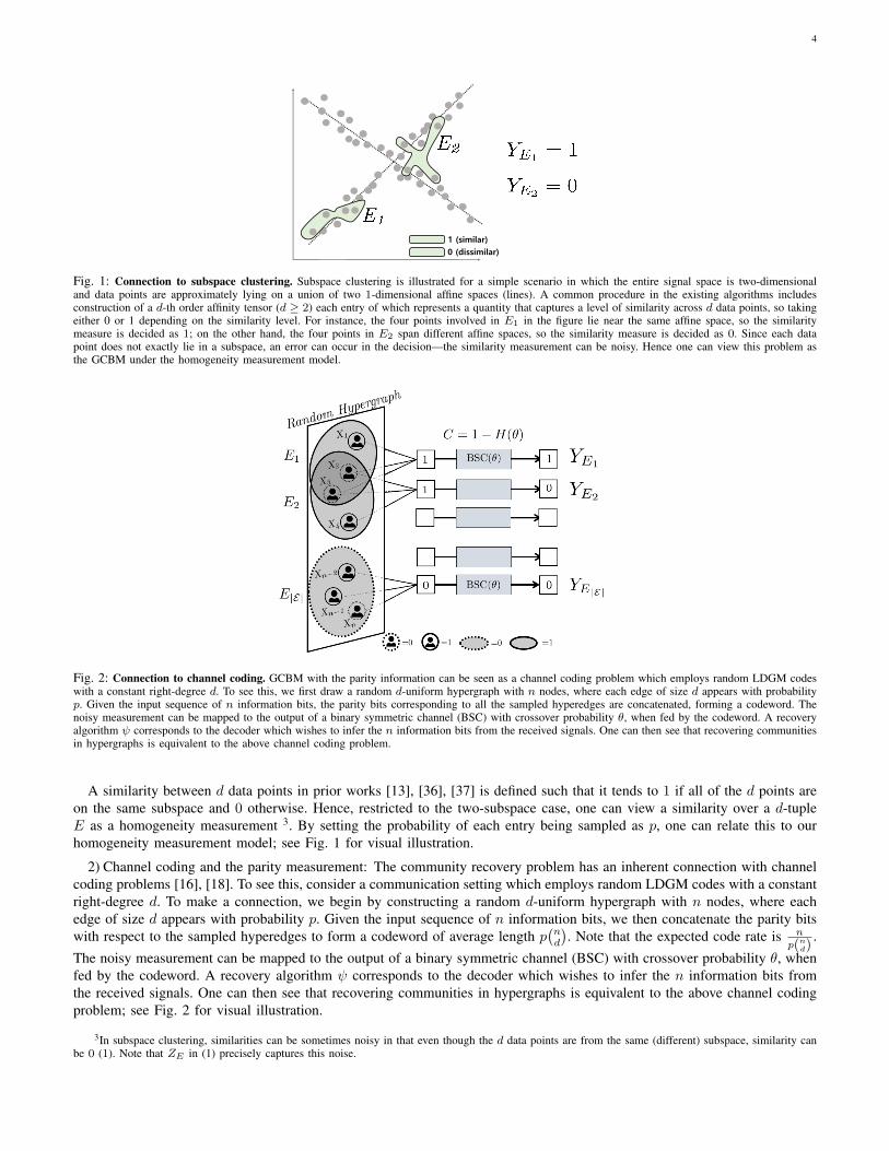
1) Subspace clustering and the homogeneity measurement: Subspace clustering is a popular problem of which the task isto cluster n data points that approximately lie in a union of lower-dimensional affine spaces. The problem arises in a varietyof applications such as motion segmentation [47] and face clustering [48], where data points corresponding to the same class(tracked points on a moving object or faces of a person) lie on a single lower-dimensional subspace; for details, see [49] andreferences therein. A common procedure of the existing algorithms for subspace clustering [37], [50]–[52] begins constructionof a d-th order affinity tensor (d ≥ 2) whose entries represent similarities between every d data points. Since this constructionincurs a complexity that scales like nd, sampling-based approaches are proposed in [13], [36], [37].
4
1 (similar)
0 (dissimilar)
Fig. 1: Connection to subspace clustering. Subspace clustering is illustrated for a simple scenario in which the entire signal space is two-dimensionaland data points are approximately lying on a union of two 1-dimensional affine spaces (lines). A common procedure in the existing algorithms includesconstruction of a d-th order affinity tensor (d ≥ 2) each entry of which represents a quantity that captures a level of similarity across d data points, so takingeither 0 or 1 depending on the similarity level. For instance, the four points involved in E1 in the figure lie near the same affine space, so the similaritymeasure is decided as 1; on the other hand, the four points in E2 span different affine spaces, so the similarity measure is decided as 0. Since each datapoint does not exactly lie in a subspace, an error can occur in the decision—the similarity measurement can be noisy. Hence one can view this problem asthe GCBM under the homogeneity measurement model.
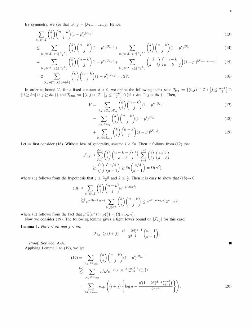
Fig. 2: Connection to channel coding. GCBM with the parity information can be seen as a channel coding problem which employs random LDGM codeswith a constant right-degree d. To see this, we first draw a random d-uniform hypergraph with n nodes, where each edge of size d appears with probabilityp. Given the input sequence of n information bits, the parity bits corresponding to all the sampled hyperedges are concatenated, forming a codeword. Thenoisy measurement can be mapped to the output of a binary symmetric channel (BSC) with crossover probability θ, when fed by the codeword. A recoveryalgorithm ψ corresponds to the decoder which wishes to infer the n information bits from the received signals. One can then see that recovering communitiesin hypergraphs is equivalent to the above channel coding problem.
A similarity between d data points in prior works [13], [36], [37] is defined such that it tends to 1 if all of the d points areon the same subspace and 0 otherwise. Hence, restricted to the two-subspace case, one can view a similarity over a d-tupleE as a homogeneity measurement 3. By setting the probability of each entry being sampled as p, one can relate this to ourhomogeneity measurement model; see Fig. 1 for visual illustration.
2) Channel coding and the parity measurement: The community recovery problem has an inherent connection with channelcoding problems [16], [18]. To see this, consider a communication setting which employs random LDGM codes with a constantright-degree d. To make a connection, we begin by constructing a random d-uniform hypergraph with n nodes, where eachedge of size d appears with probability p. Given the input sequence of n information bits, we then concatenate the parity bitswith respect to the sampled hyperedges to form a codeword of average length p
(nd
). Note that the expected code rate is n
p(nd).
The noisy measurement can be mapped to the output of a binary symmetric channel (BSC) with crossover probability θ, whenfed by the codeword. A recovery algorithm ψ corresponds to the decoder which wishes to infer the n information bits fromthe received signals. One can then see that recovering communities in hypergraphs is equivalent to the above channel codingproblem; see Fig. 2 for visual illustration.
3In subspace clustering, similarities can be sometimes noisy in that even though the d data points are from the same (different) subspace, similarity canbe 0 (1). Note that ZE in (1) precisely captures this noise.

5
III. MAIN RESULTS
A. The homogeneity measurement case
Theorem 1. Fix d ≥ 2 and ε > 0. Under the homogeneity measurement case (f = fh),infψ Pe(ψ)→ 0 if(nd
)p ≥ (1 + ε) 2d−2
dn logn
(√
1−θ−√θ)2
;
infψ Pe(ψ) 6→ 0 if(nd
)p ≤ (1− ε) 2d−2
dn logn
(√
1−θ−√θ)2.
Proof: See Sec. IV.We first make a comparison to the result in [34]. While [34] models a fairly general similarity measurement, it considers a
more relaxed performance metric, so called almost exact recovery, which allows a vanishing fraction of misclassified nodes;and provides a sufficient condition on sample complexity under the setting [53]. On the other hand, we identify the sufficientand necessary condition for exact recovery, thereby characterizing the fundamental limit. Specializing their result to the modelof our interest, the sufficient condition in [34] reads Ω(n log2 n), which comes with an extra log n factor gap to the optimality.
One interesting observation in Theorem 1 is that the sample complexity limit is proportional to 2d−2
d . This suggests thatthe amount of information that one hyperedge reveals on average is approximately d
2d−2 bits. To understand why this is thecase, consider a setting in which θ = 0 and an hyperedge E = i1, i2, · · · , id is observed. The case of YE = 1 impliesXi1 = Xi2 = · · · = Xid , in which there are only two uncertain cases (all zeros and all ones), i.e., the d−1 bits of informationare revealed. On the other hand, the case of YE = 0 provides much less information as it rules out only two possible cases(Xi1 = Xi2 = · · · = Xid = 0 and Xi1 = Xi2 = · · · = Xid = 1) out of 2d possible candidates. This amounts to roughly d · 2
2d
bits. Since YE = 1 occurs with probability 12d−1 , the amount of information that one hyperedge can carry on average should
read about 12d−1 (d− 1) +
(1− 1
2d−1
)d
2d−1 ≈ d2d−2 .
Relying on the connection to subspace clustering elaborated in Sec. II-A, one can make an interesting implication fromTheorem 1. The result offers a detailed guideline as to how to choose d for sample-efficient subspace clustering. In the casewhere the measurement quality reflected in θ is irrelevant of the number d of data points involved in a measurement, the limitincreases in d. In practical applications, however, θ may depend on d. Actually, the quality of similarity measure can improveas more data points get involved, making θ decrease as d increases. In this case, choosing d as small as possible minimizes2d−2
d but may make θ too large. Hence, there might be a sweet spot on d that minimizes the sample complexity. It turns outthis is indeed the case in practice. Actually we identify such optimal d∗ for motion segmentation application; see Sec. VII-Afor details.
B. The parity measurement case
Theorem 2. Fix d ≥ 2 and ε > 0. Under the parity measurement case (f = fp),infψ Pe(ψ)→ 0 if
(nd
)p ≥ (1 + ε) 1
dn logn
(√
1−θ−√θ)2
;
infψ Pe(ψ) 6→ 0 if(nd
)p ≤ (1 + ε) 1
dn logn
(√
1−θ−√θ)2
.
Proof: See Sec.V.Notice that for a fixed θ and n, the minimum sample complexity is proportional to 1
d , hence decreases in d unlike thehomogeneity measurement case.
In view of the connection made in Sec. II-A, a natural question that arises in the context of channel coding is to ask howfar the rate of the random LDGM code is from the capacity of the BSC channel. The connection can help immediately answerthe question. We see from Theorem 2 that the rate of the LDGM code is
n
p(nd
) =d(√
1− θ −√θ)2
log n.
This suggests that the code rate increases in d. Note that as long as d is constant, the rate vanishes, being far from the capacityof BSC channel 1 − H(θ). On the other hand, it is not clear as to whether or not the random LDGM code can achieve anon-vanishing code rate possibly by increasing the value of d. To check this, we explore the case where d can scale with n.By symmetry, it suffices to consider the case 2 ≤ d ≤ n/2. Moreover, to avoid pathological cases where d fluctuates as nincreases, we assume that d is a monotone function.
Theorem 3. Fix d, a monotone function of n such that 2 ≤ d ≤ n/2, and ε > 0. Under the parity measurement case (f = fp),• (upper bound) infψ Pe(ψ)→ 0 if (
n
d
)p ≥ (1 + ε)
5/2
d
n log n
(√
1− θ −√θ)2
and (2)(n
d
)p ≥ (1 + ε)5 log 2
n
(√
1− θ −√θ)2
; (3)

6
• (lower bound) infψ Pe(ψ) 6→ 0 if (n
d
)p ≤ (1− ε)1
d
n log n
(√
1− θ −√θ)2
or (4)(n
d
)p ≤ n
1−H(θ). (5)
Proof: See Sec. VI.To see what these results mean, consider the two cases: d = Ω(log n) and d = o(log n). In the case d = Ω(log n), the
theorem says that for a fixed θ,
infψPe(ψ)→ 0 if
(n
d
)p > β1n and
infψPe(ψ) 6→ 0 if
(n
d
)p < β2n ,
where β1 = max
5/2 logn
(√
1−θ−√θ)2d
, 5 log 2
(√
1−θ−√θ)2
1 and β2 = max
logn
(√
1−θ−√θ)2d
, 11−H(θ)
1. This suggests that as long
as d grows asymptotically larger than log n, we can achieve an order-wise tight sample complexity that is linear in n. On theother hand, in the case d = o(log n), the theorem asserts that
infψPe(ψ)→ 0 if
(n
d
)p >
5/2
d
n log n
(√
1− θ −√θ)2
and
infψPe(ψ) 6→ 0 if
(n
d
)p <
1
d
n log n
(√
1− θ −√θ)2
.
This implies that one cannot achieve the linear-order sample complexity if d grows slower than log n. The implication of theabove two can be formally stated as follows.
Corollary 1. For d = o(log n), reliable recovery is impossible with linear-order sample complexity, while it is possible ford = Ω(log n).
From this, we see that the random LDGM code can achieve a constant rate as soon as d = Ω(log n).
IV. PROOF OF THEOREM 1
The achievability and converse proofs are streamlined with the help of Lemmas 1 and 2, of which the proofs are leftin Appendix A. For illustrative purpose, we focus on the noisy case (θ > 0) and assume that n is even. For a vectorV := Vi1≤i≤n ∈ 0, 1n, we define
fi1,i2,··· ,id(V) := f(Vi1 , Vi2 , · · · , Vid);
F(V) := fE(V)E∈E ;dH(V) := ‖Y − F(V)‖1 .
(6)
Let ψML be the maximum likelihood (ML) decoder. One can easily verify that
ψML(Y) = arg minV∈0,1n
dH(V),
where ties are randomly broken.
A. Achievability proof
We intend to prove that
maxX∈0,1n
Pr(ψML(Y) /∈ X,X⊕ 1)→ 0
under the claimed condition. Let A ∈ 0, 1n be the ground-truth vector. Without loss of generality, assume that the first kcoordinates are 0’s and the next n− k coordinates are 1’s, where 0 ≤ k ≤ n/2.
Let Ai,j denote the collection of all vectors whose coordinates are different from that of A in i many positions among thefirst k coordinates and in j many positions among the next n−k coordinates. Note that A0,0 = A and Ak,n−k = A⊕1.Thus, a decoding algorithm ψ is successful if and only if the output ψ(Y) ∈ A0,0 ∪ Ak,n−k. Let I := (i, j) : (i, j) /∈(0, 0), (k, n− k), 0 ≤ i ≤ k, and 0 ≤ j ≤ n− k. We also define
Vi,j := (1, · · · , 1︸ ︷︷ ︸i
, 0, · · · , 0
︸ ︷︷ ︸k
, 0, · · · , 0︸ ︷︷ ︸j
, 1, · · · , 1
︸ ︷︷ ︸n−k
) ,

7
which is a representative vector of Ai,j .Using these notations and the union bound, we get:
Pr(ψML(Y) /∈ X,X⊕ 1 | X = A)
(a)
≤ Pr
⋃(i,j)∈I
⋃V∈Ai,j
[dH(V) ≤ dH(A)]
≤
∑(i,j)∈I
∑V∈Ai,j
Pr (dH(V) ≤ dH(A))
=∑
(i,j)∈I
(k
i
)(n− kj
)Pr (dH(Vi,j) ≤ dH(A)) , (7)
where the step (a) follows from the fact that the ML decoder outputs V /∈ A,A⊕ 1 if dH(V) ≤ dH(A).To compare dH(Vi,j) with dH(A), we define the set of distinctive hyperedges, i.e., the set of hyperedges such that fE(A) 6=
fE(Vi,j):
Fi,j :=
E ∈
([n]
d
): fE(A) 6= fE(Vi,j)
(8)
and Ei,j := E∩Fi,j . By definition, for E ∈ Ei,j , YE = fE(A) if ZE = 0; YE = fE(Vi,j) otherwise. Hence, dH(Vi,j) ≤ dH(A)
if and only if∑E∈Ei,j ZE ≥
|Ei,j |2 . This leads to:
Pr (dH(Vi,j) ≤ dH(A))
=
|Fi,j |∑`=1
Pr (dH(Vi,j) ≤ dH(A) | |Ei,j | = `) Pr(|Ei,j | = `) (9)
=
|Fi,j |∑`=1
Pr
∑E∈Ei,j
ZE ≥`
2
∣∣∣∣ |Ei,j | = `
· (|Fi,j |`
)p`(1− p)|Fi,j |−`
(a)
≤|Fi,j |∑`=1
e−`D(0.5‖θ)(|Fi,j |`
)p`(1− p)|Fi,j |−`
= (1− (1− e−D(0.5‖θ))p)|Fi,j | , (10)
where (a) is due to Chernoff-Hoeffding [54]. By letting p′ := (1− e−D(0.5‖θ))p and applying this to (7), we get:
Pr(ψML(Y) /∈ X,X⊕ 1 | X = A)
≤∑
(i,j)∈I
(k
i
)(n− kj
)(1− p′)|Fi,j |. (11)
To give a tight upper bound on (11), one needs a tight lower bound on the size of the set of distinctive hyperedges, i.e.,|Fi,j |. It turns out that bounding |Fi,j | when d > 2 requires non-trivial combinatorial counting. Note that this was not thecase when d = 2 since |Fi,j | can be exactly computed via simple counting. Indeed, one of our main technical contributionslies in the derivation of tight bounds on |Fi,j |, which we detail below.
Fact 1. The number of distinctive hyperedges can be calculated as follows:
|Fi,j | =d−1∑`=1
(i
`
)(k − id− `
)+
d−1∑`=1
(j
`
)(n− k − jd− `
)+
d−1∑`=1
(i
`
)(n− k − jd− `
)+
d−1∑`=1
(k − i`
)(j
d− `
). (12)
Proof: Consider a hyperedge E = i1, i2, · · · , id such that fE(A) = 1. That is, the hyperedge is connected onlyto a subset of the first k nodes or only to a subset of the last n − k nodes. That is, i1, i2, · · · , id ⊂ 1, 2, · · · , k ori1, i2, · · · , id ⊂ k + 1, k + 2, · · · , n. Consider the first case, i.e., i1, i2, · · · , id ⊂ 1, 2, · · · , k. In order for thishyperedge to be distinctive, i.e., fE(Vi,j) = 0, at least one element of E must be in 1, 2, · · · , i, and at least one elementof E must be in i + 1, · · · , k. Thus, the total number of such distinctive hyperedges is
∑d−1`=1
(i`
)(k−id−`). Similarly, one
can count the number of distinctive hyperedges for the case i1, i2, · · · , id ⊂ k + 1, k + 2, · · · , n:∑d−1`=1
(j`
)(n−k−jd−`
). By
considering the opposite case where fE(A) = 0 and fE(Vi,j) = 1, one can also obtain the remaining two terms, proving thestatement.
8
By symmetry, we see that |Fi,j | = |Fk−i,n−k−j |. Hence,∑(i,j)∈I
(k
i
)(n− kj
)(1− p′)|Fi,j | (13)
≤∑
(i,j)∈I, j≤bn−k2 c
(k
i
)(n− kj
)(1− p′)|Fi,j | +
∑(i,j)∈I, j≥dn−k2 e
(k
i
)(n− kj
)(1− p′)|Fi,j | (14)
=∑
(i,j)∈I, j≤bn−k2 c
(k
i
)(n− kj
)(1− p′)|Fi,j | +
∑(i,j)∈I, j≤bn−k2 c
(k
k − i
)(n− k
n− k − j
)(1− p′)|Fk−i,n−k−j | (15)
= 2∑
(i,j)∈I, j≤bn−k2 c
(k
i
)(n− kj
)(1− p′)|Fi,j | =: 2V. (16)
In order to bound V , for a fixed constant δ > 0, we define the following index sets: Ibig := (i, j) ∈ I :[j ≤ n−k
2
]∩
([i ≥ δn] ∪ [j ≥ δn]) and Ismall := (i, j) ∈ I :[j ≤ n−k
2
]∩ ([i < δn] ∩ [j < δn]). Then,
V =∑
(i,j)∈Ibig∪Ibig
(k
i
)(n− kj
)(1− p′)|Fi,j | (17)
=∑
(i,j)∈Ibig
(k
i
)(n− kj
)(1− p′)|Fi,j | (18)
+∑
(i,j)∈Ismall
(k
i
)(n− kj
)(1− p′)|Fi,j |. (19)
Let us first consider (18). Without loss of generality, assume i ≥ δn. Then it follows from (12) that
|Fi,j | ≥d−1∑`=1
(i
`
)(n− k − jd− `
)(a)
≥d−1∑`=1
(i
`
)(n/4
d− `
)≥(i
1
)(n/4
d− 1
)≥ δn
(n/4
d− 1
)= Ω(nd),
where (a) follows from the hypothesis that j ≤ n−k2 and k ≤ n
2 . Then it is easy to show that (18)→ 0:
(18) ≤∑
(i,j)∈I
(k
i
)(n− kj
)e−p
′Ω(nd)
(a)= e−Ω(n logn)
∑(i,j)∈I
(k
i
)(n− kj
)≤ e−Ω(n logn)2n → 0,
where (a) follows from the fact that p′Ω(nd) p(nd
)= Ω(n log n).
Now we consider (19). The following lemma gives a tight lower bound on |Fi,j | for this case:
Lemma 1. For i < δn and j < δn,
|Fi,j | ≥ (i+ j) · (1− 2δ)d−1
2d−2
(n− 1
d− 1
).
Proof: See Sec. A-A.Applying Lemma 1 to (19), we get:
(19) =∑
(i,j)∈Ismall
(k
i
)(n− kj
)(1− p′)|Fi,j |
(a)
≤∑
(i,j)∈Ismall
ninje−p′(i+j)· (1−2δ)d−1
2d−2 (n−1d−1)
=∑
(i,j)∈Ismall
exp
((i+ j)
log n−
p′(1− 2δ)d−1(n−1d−1
)2d−2
), (20)

9
where (a) follows due to(ki
)≤ ni,
(n−kj
)≤ nj and Lemma 1. A straightforward computation yields (1 − e−DKL(0.5‖θ)) =
(√
1− θ −√θ)2, so the claimed condition(
n
d
)p ≥ (1 + ε)
2d−2
d
n log n
(√
1− θ −√θ)2
becomes (n
d
)p′ ≥ (1 + ε)
2d−2
dn log n . (21)
Under the claimed condition, we get:
p′(1− 2δ)d−1(n−1d−1
)2d−2
=p′(1− 2δ)d−1
(nd
)dn
2d−2
(a)
≥ (1 + ε)(1− 2δ)d−1 log n
(b)
≥ (1 + ε/2) log n,
where (a) follows from (21); (b) follows by choosing δ sufficiently small ((1− 2δ)d−1 → 0 as δ → 0). Thus, (20) convergesto 0 as n tends to infinity. This completes the proof.
B. Converse proof
Let V1/2 be the collection of n-dimensional vectors, each consisting of n/2 number of 0’s and n/2 number of 1’s. Moreover,let X1/2 be the random vector sampled uniformly at random over V1/2. For any scheme ψ, by definition of Pe(ψ), we seethat
Pr(ψ(Y) /∈ X, X⊕ 1 | X = X1/2
)≤ Pe(ψ)
and hence
infψ
Pr(ψ(Y) /∈ X, X⊕ 1 | X = X1/2
)≤ inf
ψPe(ψ).
Relying on this inequality, our proof strategy is to show that the left hand side is strictly bounded away from 0. Note that theinfimum in the left hand side is achieved by ψML,1/2:
ψML,1/2(Y) = arg minV∈V1/2
dH(V) .
By letting A = (0, · · · , 0︸ ︷︷ ︸n/2
, 1, · · · , 1︸ ︷︷ ︸n/2
), we obtain
Pr(ψML,1/2(Y) /∈ X, X⊕ 1 | X = X1/2
)= Pr
(ψML,1/2(Y) /∈ A, A⊕ 1 | X = A
).
Let S be the success event:
S :=⋂
V∈V1/2\A,A⊕1
[dH(V) > dH(A)] .
One can show that Pr(ψML,1/2(Y) /∈ A, A⊕ 1 | X = A
)≥ 1
3 Pr(Sc). This is due to the fact that given Sc, there aremore than two candidates for arg minV∈V1/2 dH(V), so
Pr(ψML,1/2(Y) /∈ A, A⊕ 1 | X = A, Sc
)≥ 1
3.
Hence, it suffices to show Pr(S)→ 0. To give a tight upper bound on Pr(S), we construct a subset of nodes such that any twonodes in the subset do not share the same hyperedge. To this end, we use the deletion technique (alteration technique) [55].We first choose a big subset
Rbig = 1, 2, · · · , r⋃n
2+ 1,
n
2+ 2, · · · , n
2+ r,
where r = d nlog7 n
e; then erase every node in Rbig which shares hyperedges with other nodes in Rbig to obtain Rres. Thefollowing lemma guarantees that Rres has a comparable size as that of Rbig with high probability. For the later usage, weallow d to scale with n.

10
Lemma 2. Suppose(nd
)p = O(n log n) and d = O(log n). Let Rbig be a subset of [n] and Rres be a subset obtained from
Rbig by deleting every node which shares hyperedges with other nodes in Rbig. If |Rbig| = O(n/ log7 n), then with probabilityapproaching 1,
|Rres| = (1− o(1))|Rbig| .
Proof: See Sec. A-B.Let ∆ be the event that |Rres| ≥ (1−o(1))|Rbig|. Given the event ∆, both 1, 2, · · · , n/2∩Rres and
n2 + 1, n2 + 2, · · · , n
∩
Rres contain more than r/2 elements. We collect r/2 elements from each of these sets and denote by b1, b2, · · · , br/2 andc1, c2, · · · , cr/2, respectively. Suppose that there exist (k, `) such that dH(A ⊕ ebk) ≤ dH(A) and dH(A ⊕ ec`) ≤ dH(A).Conditioning on ∆, there are no hyperedges that contain both bk and c`, so dH(A⊕ ebk ⊕ ec`) ≤ dH(A). Hence conditioningon ∆,
S ⊂r/2⋂k=1
[dH(A⊕ ebk) > dH(A)]⋃ r/2⋂
k=1
[dH(A⊕ eck) > dH(A)]
=: S′.
Since the event ∆ occurs with probability approaching 1 and S ⊂ S′, Pr(S) ' Pr(S | ∆) ≤ Pr(S′ | ∆). Hence,
Pr(S) . Pr (S′ | ∆)
≤ 2 Pr
r/2⋂k=1
[dH(A⊕ ebk) > dH(A)]
∣∣∣∣ ∆
(a)= 2 Pr
(dH(A⊕ eb1) > dH(A)
∣∣ ∆)r/2
,
where (a) follows from the fact that the events [dH(A⊕ebk) > dH(A)]1≤k≤r/2 are mutually independent conditioned on ∆.Let p′ = (1−e−DKL(0.5‖θ))p as in the achievability proof. We intend to give an upper bound on Pr
(dH(A⊕ eb1) > dH(A)
∣∣ ∆),
i.e., a lower bound on Pr(dH(A⊕ eb1) ≤ dH(A)
∣∣ ∆). Recall from the proof of achievability (see (10)) that
Pr (dH(Vi,j) ≤ dH(A)) ≤ (1− (1− e−DKL(0.5‖θ))p)|Fi,j | .
For the case of Vi,j = A⊕ eb1 , |Fi,j | =(n/2−1d−1
)+(n/2d−1
)(note that k = n/2, i = 1, j = 0). So we get:
Pr (dH(A⊕ eb1) ≤ dH(A)) ≤ e−p′((n/2−1
d−1 )+(n/2d−1)) . (22)
On the other hand, what we need for the converse proof is a lower bound. In what follows, we will show that (22) is tightenough, more precisely,
Pr(dH(A⊕ eb1) ≤ dH(A)
∣∣ ∆)≥ (1− o(1))e−2p′(n/2−1
d−1 ) . (23)
What this means at a high level is that Chernoff-Hoeffding is tight enough. Let us condition on the event ∆ for the timebeing. As in (8), we define the following sets:
Fb1 :=
E ∈
([n]
d
): fE(A) 6= fE(A⊕ eb1)
and Eb1 := E ∩ Fb1 . By definition, for E ∈ Eb1 , YE = fE(A) if ZE = 0; YE = fE(A⊕ eb1) otherwise. We see that
dH(A⊕ eb1) ≤ dH(A)⇔∑E∈Eb1
ZE ≥|Eb1 |
2.
Now we want to manipulate Pr(dH(A⊕ eb1) ≤ dH(A)
∣∣ ∆)
as we did in (9). However, here we need to give a carefulattention to the range of summation as Eb1 cannot be equal to Fb1 due to the following reason. Since we conditioned on ∆,no hyperedge in Eb1 intersects Rbig at more than one node (indeed, b1 is the only node where they intersect); in other words,Eb1 is always contained in a proper subset of Fb1 :
Eb1 ⊂ Fb1 \E ∈
([n]
d
): |E ∩Rbig| ≥ 2
=: Gb1 . (24)
Now a manipulation similar to (9) yields:
Pr (dH(A⊕ eb1) ≤ dH(A) | ∆)
=
|Gb1 |∑`=1
Pr(dH(A⊕ eb1) ≤ dH(A)
∣∣ |Eb1 | = `, ∆)
Pr(|Eb1 | = `|∆).

11
Since the event ∆ is related to the occurrence of edges inE ∈
([n]
d
): |E ∩Rbig| ≥ 2
and Eb1 is subject to (24), ∆ and [|Eb1 | = `] are independent. Thus, we get:
Pr (dH(A⊕ eb1) ≤ dH(A) | ∆)
=
|Gb1 |∑`=1
Pr(dH(A⊕ eb1) ≤ dH(A)
∣∣ |Eb1 | = `, ∆)
Pr(|Eb1 | = `)
=
|Gb1 |∑`=1
Pr
∑E∈Eb1
ZE ≥`
2
∣∣∣∣|Eb1 | = `
(|Gb1 |`
)p`
(1− p)`−|Gb1 |. (25)
By the reverse Chernoff-Hoeffding bound [54], for a fixed δ > 0, there exists nδ > 0 such that
Pr
∑E∈Eb1
ZE ≥`
2
∣∣∣∣|Eb1 | = `
≥ e−(1+δ)`DKL(0.5‖θ)
for all ` ≥ nδ . Let gn be a sequence (to be determined) such that gn →∞ as n→∞. For sufficiently large n,
(25) ≥|Gb1 |∑`=1
(|Gb1 |`
)(e−(1+δ)DKL(0.5‖θ)p)`
(1− p)`−|Gb1 |(26)
−gn−1∑`=1
(|Gb1 |`
)(e−(1+δ)DKL(0.5‖θ)p)`
(1− p)`−|Gb1 |. (27)
Actually one can choose gn so that (27) is negligible compared to (26). To see this, we consider:
(27)(26)
≤(1− p)|Gb1 |
∑gn−1`=1
(|Gb1 |
pe−(1+δ)DKL(0.5‖θ)
1−p
)`(1− p)|Gb1 |
∑|Gb1 |`=1
(|Gb1 |`
) (pe−(1+δ)DKL(0.5‖θ)
1−p
)`=
∑gn−1`=1
(|Gb1 |
pe−(1+δ)DKL(0.5‖θ)
1−p
)`(
1 + pe−(1+δ)DKL(0.5‖θ)
1−p
)|Gb1 |(a)=
∑gn−1`=1
(|Gb1 |
pe−(1+δ)DKL(0.5‖θ)
1−p
)`(1 + o(1)) exp
(|Gb1 |
pe−(1+δ)DKL(0.5‖θ)
1−p
)=:
∑gn−1`=1 q`
(1 + o(1))eq, (28)
where (a) follows from the fact that limx→0+1+xex = 1, and the last equation is due to the following definition: q :=
|Gb1 |pe−(1+δ)DKL(0.5‖θ)
1−p . One can easily verify that |Fb1 | =(n/2−1d−1
)+(n/2d−1
)and |Gb1 | =
(n/2−1−rd−1
)+(n/2−rd−1
). Since r = o(n),
limn→∞ |Gb1 |/|Fb1 | → 1. Thus,
q = |Gb1 |pe−(1+δ)DKL(0.5‖θ)
1− p(29)
|Fb1 |pe−(1+δ)DKL(0.5‖θ)
1− p nd−1p = Ω(log n) . (30)
Therefore, if one chooses gn = blog qc,
(27)(26)
=
∑gn−1`=1 q`
eq≤ gnq
gn
eq≤ log q · qlog q
eq=
log q · e(log q)2
eq→ 0,
and thus (27) = o(1) · (26).

12
Hence, we get:
(25) = (26)− (27)
≥ (1− o(1))
|Gb1 |∑`=1
(|Gb1 |`
)(e−(1+δ)DKL(0.5‖θ)p)`
(1− p)`−|Gb1 |
= (1− o(1))(
1− (1− e−(1+δ)DKL(0.5‖θ))p)|Gb1 |
(a)
≥ (1− o(1))(
1− (1− e−(1+δ)DKL(0.5‖θ))p)2(n/2d−1)
(b)= (1− o(1)) exp
(−2
(n/2
d− 1
)(1− e−(1+δ)DKL(0.5‖θ))p
),
where (a) follows since |Gb1 | ≤ |Fb1 | ≤ 2(n/2d−1
); (b) follows from the fact that limx→0+
1+xex = 1. As δ > 0 can be chosen
arbitrarily small, the term e−(1+δ)DKL(0.5‖θ) can be made arbitrarily close to e−DKL(0.5‖θ), which in turn ensures that the lastterm is essentially equal to
(1− o(1))e−2p′(n/2d−1).
Applying this to the previous upper bound on Pr(S), we get:
Pr(S) ≤ Pr(dH(A⊕ eb1) > dH(A)
∣∣ ∆)r/2
≤(
1− (1− o(1))e−2p′(n/2d−1))r/2
≤ exp(−(1− o(1))
r
2e−2p′(n/2d−1)
)= exp
(−(1− o(1))
n
2 log7 ne−(1+o(1))·
p′d(nd)2d−2n
),
where the last equality follows from the fact that
limn→∞
2p′(n/2d−1
)p′d(nd
)/2d−2n
→ 1 and r =
⌈n
log7 n
⌉.
The last term converges to 0 as p′ ≤ (1− ε) 2d−2
dn logn
(nd).
V. PROOF OF THEOREM 2
In this section, we prove a similar statement for the parity measurement case.
A. Achievability proof
Note that the parity measurement is symmetric in a sense that for any two vector A and B, Pr (ψML(Y) /∈ X, X⊕ 1 | X = A) =Pr (ψML(Y) /∈ X, X⊕ 1 | X = B). Hence, we will prove that
Pr (ψML(Y) /∈ X, X⊕ 1 | X = 0)→ 0

13
under the claimed condition. Conditioning on X = 0,
Pr (ψML(Y) /∈ 0,1)
≤ Pr
⋃A 6=0,1
[dH(A) ≤ dH(0)]
= Pr
n−1⋃k=1
⋃‖A‖1=k
[dH(A) ≤ dH(0)]
≤n−1∑k=1
∑‖A‖1=k
Pr (dH(A) ≤ dH(0))
(a)= 2 ·
n/2∑k=1
∑‖A‖1=k
Pr (dH(A) ≤ dH(0))
(b)= 2 ·
n/2∑k=1
(n
k
)Pr
(dH
(k∑i=1
ei
)≤ dH(0)
), (31)
where (a) follows form the fact that Pr (dH(A) ≤ dH(0)) = Pr (dH(A⊕ 1) ≤ dH(0)); (b) follows due to symmetry. Tocompare dH
(∑ki=1 ei
)and dH(0), we define
Fk :=
E ∈
([n]
d
): fE(0) 6= fE
(k∑i=1
ei
)and Ek := E ∩ Fk. As in (10), we obtain
Pr
(dH
(k∑i=1
ei
)≤ dH(0)
)≤ (1− (1− e−DKL(0.5‖θ))p)|Fk|
= (1− p′)|Fk| ,
yielding
1
2· (31) ≤
n/2∑k=1
(n
k
)(1− p′)|Fk|. (32)
We again count |Fk| in an effort to obtain a tight upper bound on (32). Notice that E ∈ Fk if |E ∩ [k]| is odd, and hence
|Fk| =∑i≤di is odd
(k
i
)·(n− kd− i
). (33)
Let δ > 0 be a small constant that will be determined later. For the case k ≥ δn, it follows that
|Fk| ≥(k
1
)(n− kd− 1
)≥ δn
(n/2
d− 1
)= Ω(nd) .
Then it is easy to show (32)→ 0 for this case:
n/2∑k=δn
(n
k
)(1− p′)|Fk| ≤
n/2∑k=δn
(n
k
)e−p
′Ω(nd)
(a)= e−Ω(n logn)
n/2∑k=δn
(n
k
)≤ e−Ω(n logn)2n → 0 ,
where (a) follows from the fact that p′Ω(nd) p(nd
)= Ω(n log n). For the case k < δn, we see that
|Fk| ≥(k
1
)(n− kd− 1
)≥ k
((1− δ)nd− 1
)(a)=
n→∞(1 + o(1))k(1− δ)d−1
(n− 1
d− 1
), (34)

14
where (a) follows since
limn→∞
αd−1(n−1d−1
)(αnd−1
) = 1 (35)
holds for a fixed d and α ∈ (0, 1). Hence, we get
δn∑k=1
(n
k
)(1− p′)|Fk| ≤
δn∑k=1
nke−(1+o(1))p′k(1−δ)d−1( nd−1)
=
δn∑k=1
ek·logn−(1+o(1))p′(1−δ)d−1( nd−1) . (36)
By choosing δ arbitrarily small, under the claimed condition, one can make
p′(1− δ)d−1
(n
d− 1
)= (1 + o(1))(1− δ)d−1
(n
d
)p′d
n
≥ (1 + ε/2) log n ,
which implies that (36) converges to 0 as n tends to infinity.
B. Converse proof
As the parity measurement is symmetric,
infψPe(ψ) = Pr (ψML(Y) /∈ X, X⊕ 1 | X = 0) .
As before, we define the success event as:
S :=⋂
V 6=0,1
[dH(V) > dH(0)] . (37)
Again, it suffices to show that Pr(S) → 0, and to this end, we construct a subset of nodes such that any two nodes in thesubset do not share the same hyperedge. Unlike the previous case, the subset is now defined as:
Rbig := 1, 2, · · · , r (38)
where r = d nlog7 n
e, and we erase every node in Rbig which shares hyperedges with other nodes in Rbig to obtain Rres. Inview of Lemma 2, we have |Rres| ≥ (1− o(1))r almost surely; let ∆ be such event. Conditioning on ∆, we enumerate r/2many elements of Rres by b1, · · · , br/2. As there are no hyperedges that connect two nodes in Rres, the events [dH(ebk) >dH(0)]1≤k≤r/2 are mutually independent conditioned on ∆. Hence, we get:
Pr(S) . Pr (S | ∆)
≤ Pr
r/2⋂k=1
[dH(ebk) > dH(0)]
∣∣∣∣ ∆
= Pr
(dH(eb1) > dH(0)
∣∣ ∆)r/2
. (39)
Let p′ = (1− e−DKL(0.5‖θ))p as before. Using similar arguments used in the previous section, we have
Pr(dH(eb1) ≤ dH(0)
∣∣ ∆)≥ (1− o(1))e−p
′(n−1d−1) . (40)
This gives:
Pr(dH(eb1) > dH(0)
∣∣ ∆)r/2
≤(
1− (1− o(1))e−p′(n−1d−1)
)r/2≤ exp
(−(1− o(1))
r
2exp
−p′(n− 1
d− 1
))≤ exp
(−(1− o(1))
n
2 log7 nexp
−(1 + o(1)) ·
p′(nd
)d
n
).
Notice that the last term converges to 0 as(nd
)p′ ≤ (1− ε)n logn
d , which completes the proof.

15
VI. PROOF OF THEOREM 3
When d scales with n, a technical challenge arises, and we will focus on such technical difficulties, skipping most of theredundant parts.
A. Proof of the upper bound
From (32) and (33), we get
Pe(ψML) ≤n/2∑k=1
(n
k
)(1− p′)Nk , (41)
where
Nk :=∑
1≤i≤di is odd
(k
i
)·(n− kd− i
)(42)
and p′ := (√
1− θ −√θ)2p. Let us focus on counting Nk. When d 1,
(nd
)≈ nd
d! suffices to obtain a proper bound on Nk.However, in the general case where d scales with n, one needs a more delicate bounding technique to obtain sharp results.The following lemma presents our new bound.
Lemma 3. Let β := dn−d+12d+1 e < n/2 and α := n−d+1
d . Then
∑1≤i≤di is odd
(k
i
)(n− kd− i
)≥
2k5α
(nd
), k < β;
15
(nd
), β ≤ k ≤ n/2 .
Proof: See Sec. VI-C. The proof requires an involved combinatorial counting, which is one of our main technicalcontributions.
Employing Lemma 3, we get:
(41) ≤β−1∑k=1
(n
k
)(1− p′)Nk +
n/2∑k=β
(n
k
)(1− p′)Nk
≤β−1∑k=1
(n
k
)(1− p′)
2k5α (nd) +
n/2∑k=β
(n
k
)(1− p′)
15 (nd)
≤β−1∑k=1
nke−p′ 2k5α (nd) + 2ne−
15p′(nd)
≤β−1∑k=1
exp
k
(log n−
2p′(nd
)5α
)(43)
+ exp
n log 2− 1
5p′(n
d
). (44)
Note that (44) vanishes due to (3). In order to show that (43) vanishes as well, we consider two cases: d = o(n) and d n.When d = o(n),
β−1∑k=1
exp
k
(log n−
2p′(nd
)5α
)
≤β−1∑k=1
exp
k
(log n−
2dp′(nd
)5n
)
≤exp
(log n− 2dp′(nd)
5n
)1− exp
(log n− 2dp′(nd)
5n
) → 0,
since log n− 2dp′(nd)5n → −∞.

16
If d n,β−1∑k=1
exp
k
(log n−
2p′(nd
)5α
)≤ β max
1≤k≤β−1exp
k
(log n−
2p′(nd
)5α
)= β exp
(log n−
2p′(nd
)5α
),
where the last equality holds since log n− 2p′(nd)5α < 0, and hence k = 1 achieves the maximum value. Note that this vanishes
since β is asymptotically bounded by a constant. Therefore, (43) always vanishes, completing the proof.
B. Proof of the lower bound
The lower bound statement can be rewritten as follows: infψ Pe(ψ) 6→ 0 if(nd
)p ≤ max
((1− ε) 1
dn logn
(√
1−θ−√θ)2, n
1−H(θ)
).
Note that when d = ω(log n), the condition reduces to(nd
)p ≤ n
1−H(θ) . Hence, it is sufficient to show the following twostatements.• If d = O(log n): infψ Pe(ψ) 6→ 0 if
(nd
)p ≤ max
((1− ε) 1
dn logn
(√
1−θ−√θ)2, n
1−H(θ)
).
• If d = ω(log n): infψ Pe(ψ) 6→ 0 if(nd
)p ≤ n
1−H(θ) .
We first show that(nd
)p ≤ n
1−H(θ) implies infψ Pe(ψ) 6→ 0 for all d. By rearranging terms, we have(nd
)p ≤ n
1−H(θ) ⇔n
(nd)p≥ 1 −H(θ). One can immediately observe that this implies infψ Pe(ψ) 6→ 0 since n
(nd)p(which can be viewed as the
rate of a code) cannot exceed the Shannon capacity of the channel 1−H(θ).We now prove that
(nd
)p ≤ (1 − ε) 1
dn logn
(√
1−θ−√θ)2
implies infψ Pe(ψ) 6→ 0 if d = O(log n). Further, we will focus on the
case of(nd
)p n logn
d since this is the regime where the largest amount of information is available. Again, it is enough toshow that Pr(S)→ 0, where S is defined as (37). By defining Rbig,Rres,∆ and b1, · · · , br/2 as before, we again obtain (39):
Pr(S) ≤ Pr(dH(eb1) > dH(0)
∣∣ ∆)r/2
. (45)
We finish the proof by showing the following for the considered case:
Pr(dH(eb1) ≤ dH(0)
∣∣ ∆)≥ (1− o(1))e−2p′(n−1
d−1) .
While following the proof of (23), the key technical difficulty arises when checking q = Ω(log n) (see (30)): a simplecalculation yields |Fb1 | =
(n−1d−1
)and |Gb1 | =
(n−|Rbig|d−1
), but here it is not clear whether
(n−|Rbig|d−1
)(n−1d−1
)when d is not a
constant. We resolve this using a careful estimation as follows. As |Rbig| = Θ( nlog7 n
) and d = O(log n), it is straightforwardto verify
1− 1
log2 n≤n− |Rbig| − jn− 1− j
for 0 ≤ j ≤ d− 2. This simple yet crucial inequality concludes:(n−|Rbig|d−1
)(n−1d−1
) =
d−2∏j=0
n− |Rbig| − jn− 1− j
≥(
1− 1
log2 n
)d−1
≈ exp
− d− 1
log2 n
→ 1.
C. Proof of Lemma 3
Without loss of generality, we prove the lemma assuming that k ≥ d. The proof for the other cases is similar.We wish to obtain lower bounds on
Nk =∑
1≤i≤di is odd
(k
i
)(n− kd− i
)=
(k
1
)(n− kd− 1
)︸ ︷︷ ︸boundary odd term
+∑
i=1,3,··· ,d−3,d−1
(k
i
)(n− kd− i
)︸ ︷︷ ︸
intermediate odd terms
+
(k
d− 1
)(n− k
1
)︸ ︷︷ ︸
boundary odd term
(46)
in terms of(nd
). First, observe that(n
d
)=∑
0≤i≤d
(k
i
)(n− kd− i
)=
(k
0
)(n− kd
)︸ ︷︷ ︸
boundary term
+∑
i=1,2,··· ,d−2,d−1
(k
i
)(n− kd− i
)︸ ︷︷ ︸
intermediate terms
+
(k
d
)(n− k
0
)︸ ︷︷ ︸
boundary term
. (47)

17
Suppose we have the following bounds:(k
0
)(n− kd
)+
(k
d
)(n− k
0
)︸ ︷︷ ︸
sum of boundary terms
≤ A1
[(k
1
)(n− kd− 1
)+
(k
d− 1
)(n− k
1
)]︸ ︷︷ ︸
sum of boundary odd terms
; (48)
∑i=1,2,··· ,d−2,d−1
(k
i
)(n− kd− i
)︸ ︷︷ ︸
intermediate terms
≤ A2 ·∑
i=1,3,··· ,d−3,d−1
(k
i
)(n− kd− i
)︸ ︷︷ ︸
intermediate odd terms
+A3Nk , (49)
for some quantities A1, A2, A3 > 0. Then, by summing up the two inequalities, one can obtain a lower bound on Nk:(n
d
)≤ (max(A1, A2) +A3)Nk . (50)
Thus, the proof is completed as long as one can find the quantities A1, A2 and A3 that satisfy (48) and (49).We begin with (49). The following lemma asserts that A2 = 2 and A3 = 3 satisfy (49).
Lemma 4. For 1 ≤ k ≤ n/2, ∑i=1,2,··· ,d−2,d−1
(k
i
)(n− kd− i
)≤ 2 ·
∑i=1,3,··· ,d−3,d−1
(k
i
)(n− kd− i
)+ 3Nk.
Proof: See Sec. A-C.For (49), the following lemma characterizes A1.
Lemma 5. Let β :=⌈n−d+12d+1
⌉. For β ≤ k ≤ n/2,(
k
0
)(n− kd
)+
(k
d
)(n− k
0
)≤ 2
[(k
1
)(n− kd− 1
)+
(k
d− 1
)(n− k
1
)]. (51)
For k < β, (k
0
)(n− kd
)+
(k
d
)(n− k
0
)≤ α
k
[(k
1
)(n− kd− 1
)+
(k
d− 1
)(n− k
1
)](52)
andα
k≥ 2 , (53)
where α = n−d+1d .
Proof: See Sec. A-D.That is, A1 = 2 if β ≤ k ≤ n/2, and A1 = α
k if k < β.We now are ready to prove Lemma 3 with the help of Lemma 4, Lemma, 5 and (50). When β ≤ k < n/2,(
n
d
)≤ 5Nk.
When k < β, (n
d
)≤(
max(
2,α
k
)+ 3)Nk ≤
5α
2kNk,
where the last inequality holds since αk ≥ 2. This completes the proof.
VII. EXPERIMENTAL RESULTS
A. The homogeneity measurement case
1) Efficient algorithms: We also develop a computationally-efficient algorithm that achieves the information-theoretic limitcharacterized in Theorem 1. Here we only present the algorithm while deferring a detailed analysis to our companion paper [56].The algorithm operates in two stages, beginning with a decent initial estimate from Hypergraph Spectral Clustering [56]followed by iterative refinement. Detailed procedures are presented in Algorithm 1. Our algorithm is inspired by two-stageapproaches that have been applied to a wide variety of problems including matrix completion [57], [58], phase retrieval [59],[60], robust PCA [61], community recovery [18], [20], [32], [62], [63], EM-algorithm [64], and rank aggregation [65].

18
Algorithm 1
1: For E ∈(
[n]d
), define
WE :=
YE if E ∈ E ;
0, otherwise.
2: Apply Spectral Hypergraph Clustering [56] to a weighted hypergraph ([n], WEE∈([n]d )) to obtain X(0) = X(0)
i 1≤i≤n ∈0, 1n.
3: For t = 0, 1, · · · , T − 1 (T = c log n for some constant c > 0), update X(t) = X(t)i 1≤i≤n as per
X(t+1)i =
X
(t)i if dH(X(t)) < dH(X(t) ⊕ ei);
X(t)i ⊕ 1 if dH(X(t)) ≥ dH(X(t) ⊕ ei),
for i = 1, 2, · · · , n, where dH(·) is defined in (6).4: Output X(T ) = X(T )
i 1≤i≤n.
0 0.5 1 1.5 2
Normalized sample complexity
0
0.1
0.2
0.3
0.4
0.5
0.6
0.7
0.8
0.9
1
Pro
babi
lity
of s
ucce
ss
=0.01 =0.05 =0.10 =0.20
(a) Varying θ
0 0.5 1 1.5 2
Normalized sample complexity
0
0.1
0.2
0.3
0.4
0.5
0.6
0.7
0.8
0.9
1
Pro
babi
lity
of s
ucce
ss
d =3d =4d =5d =6
(b) Varying d
Fig. 3: Algorithm 1 achieves the optimal sample complexity. We run Monte Carlo simulations to estimate the probability of success when: (a) n = 1000,d = 4, and for various choices of θ; (b) n = 1000, θ = 0.05, and for various choices of d. For each curve, we normalize the number of samples by therespective information theoretic limits, characterized in Theorem 1. Observe that the probability of success quickly approaches 1 as the normalized samplecomplexity crosses 1.
2) Performance of Algorithm 1: We demonstrate the performance of Algorithm 1 by running Monte Carlo simulations.Each point plotted in Fig. 3a and Fig. 3b indicates an empirical success rate. We take 100 Monte Carlo trials. Fig. 3a showsthe probability of success when n = 1000, d = 4, and for various choices of θ. Shown in Fig. 3b is the performance of ouralgorithm with n = 1000, θ = 0.05, and for various choices of d. For both figures, the x-axis denotes the number of samplesnormalized by the respective information-theoretic limits, characterized in Theorem 1. One can observe that the successprobability due to Algorithm 1 quickly approaches 1 as the normalized sample complexity crosses 1, which corroborates ourtheoretical findings.
3) Optimal d for subspace clustering: We observe how the fundamental limit varies as a function of d. As we brieflydiscussed in Sec. III, if the noise rate θ is irrelevant to d, the optimal choice of d would be the minimum possible value ofd. However, if the noise quality θ depends on d, there may be a sweet spot for d.
We demonstrate the existence of a sweet spot in one of subspace clustering applications: motion segmentation. We usethe benchmark Hopkins 155 [66] dataset to compute an empirical noise rate θ as a function d as follows. For each sampledhyperedge E = i1, · · · , id, we adopt the method proposed in [37] to evaluate similarity between the corresponding d datapoints that we denote by D. Then, we set YE = 1 if and only if D is less than a fixed threshold, which is appropriatelychosen so that Pr(YE = 0 | i1, i2, · · · , id are from the same line) ≈ Pr(YE = 1 | i1, i2, · · · , id are not from the same line).We estimate the effective noise rate θ := Pr(YE = 0 | i1, i2, · · · , id are from the same line) for various d, and observe thatθ quickly decreases as d increases; see Fig. 4a. We then plug these θ’s to the limit characterized in Theorem 1; see Fig. 4b.Note that d = 5 is not the optimal choice, but d = 6 is the sweet spot.
We also corroborate the existence of a sweet spot in a synthetic data set for subspace clustering, shown in Fig. 5a. Here thegoal is to cluster n (= 200) 2-dimensional data points approximately lying on a union of two lines (1-dimensional subspaces).

19
5 10 15 20
Degree (d)
0
0.1
0.2
0.3
Est
imat
ed n
oise
rat
e
(a) Estimated empirical noise rate θ
5 6 7 8
Degree (d)
1
1.5
2
The
info
rmat
ion-
theo
retic
lim
it
104
(b) d∗
Fig. 4: Existence of d∗ in motion segmentation. (a) We estimate the empirical noise rate θ as a function of d in motion segmentation. (b) We plug θ tothe limit characterized in Theorem 1 and verify that d∗ = 6.
-10 -5 0 5 10
-10
-5
0
5
10
cluster 1cluster2
(a) Randomly generated data set
1000 2000 3000 4000 5000 6000
Normalized sample complexity
0
0.1
0.2
0.3
0.4
0.5
0.6
0.7
0.8
0.9
1P
roba
bilit
y of
suc
cess
d=3d=4d=5d=6
(b) Varying d
Fig. 5: Optimal choice of d when θ decays with d. We run Monte Carlo simulations to estimate the probability of success with the data set shown in(a). We observe that the effective noise rate decreases as d increases. For varying d from 3 to 6, the success probability of Algorithm 1 is shown in (b): thebest performance of the algorithm is observed when d = 4.
We compute YE as above and evaluate the performance of Algorithm 1, shown in Fig. 5b. As a result, we observe that theoptimal choice of d here is 4 rather than 3.
B. The parity measurement case
1) Efficient algorithms: For the parity measurement case, there are two efficient algorithms in the literature [38], [67].In [38], it is shown that for d = 3, a variant of message passing algorithm successfully recovers the ground-truth vectorprovided that
(n3
)p = Ω(n2/ log n). Another efficient algorithm is based on a low-rank tensor factorization algorithm proposed
in [67], and it is proved that reliable community recovery is feasible if(n3
)p = Ω(n1.5 log4 n). In either of the two cases, the
sufficient condition comes with a polynomial term (n or n1/2) to the fundamental limit characterized in Theorem 1. In fact,it is conjectured in [39] (see Conjecture 1 therein) that at least n1.5 many samples are required for exact recovery.
On the other hand, focusing on the θ = 0 case, recovering the ground-truth vector from the measurement vector Y isessentially the same as solving linear equations over the Galois field of two elements F2. Hence it immediately follows thatefficient algorithms for solving linear equations such as Gaussian elimination can be employed in the noiseless case.
2) Information-theoretic limit: We first provide Monte Carlo simulation results which corroborate our theoretical findingsin Theorem 2. Each point plotted in Fig. 6 and Fig. 7 is an empirical success rate. All results are obtained with 50 MonteCarlo trials. In Fig. 6, we plot the probability of successful recovery for n = 1000, varying d, and θ = 0. For each d, wenormalize the number of samples by max(n, n log n/d). One can observe that the probability of success quickly approaches

20
Normalized sample complexity0 0.5 1 1.5 2
Pro
babi
lity
of s
ucce
ss0
0.2
0.4
0.6
0.8
1
d = 4d = 7d = 11
Fig. 6: We run the Monte Carlo simulations to estimate the probability of success for n = 1000, varying d, and θ = 0. For each d, we normalize thenumber of samples by max(n, n logn/d). Observe that the probability of success quickly approaches 1 as the normalized sample complexity crosses 1.
Degree (d)2 4 6 8 10
Pro
babi
lity
of s
ucce
ss
0
0.1
0.2
0.3
0.4
0.5
0.6
0.7
0.8
0.9
1
n = 50n = 200n = 800n = 3200
Fig. 7: We run the Monte Carlo simulations to estimate the probability of success for varying n, varying d, θ = 0, and p = 1.1n/(nd
). Note that when n
increases by a multiplicative factor of 4, the curve shifts rightward about the same amount, supporting our result in Corollary 1
1 as the normalized sample complexity crosses 1.
3) Minimum d for linear sample complexity: Plotted in Fig. 7 are the simulation results for varying n, varying d, θ = 0,and p = 1.1n/
(nd
). We note that when n increases by a multiplicative factor of 4, the curve shifts rightward about the same
amount, supporting our result in Corollary 1.
VIII. CONCLUSION
In this paper, we investigate the problem of community recovery in hypergraphs under the two generalized censored blockmodels (GCBM), one based on the homogeneity measurement and the other based on the parity measurement. For these twomodels, we fully characterize the information-theoretic limits on sample complexity as a function of the number of nodes n,the size of edges d, the noise rate θ, and the edge observation probability p. We also corroborate our theoretical findings viaexperiments.
We conclude our paper by highlighting a few interesting open problems. One interesting question is whether or notone can sharpen Theorem 3 to characterize exact information-theoretic limits for the scaling d case. From the simulationresults in Sec. VII-B, we make the following conjecture: Under the setting of Theorem 3, the information-theoretic limitsis max
n
1−H(θ) ,1d
n logn
(√
1−θ−√θ)2
. Another interesting open problem is about the computational gap for the parity measure-
ment case: Investigating efficient algorithms for this case would shed some light on the study of information-computationgaps.
REFERENCES
[1] K. Ahn, K. Lee, and C. Suh, “Community recovery in hypergraphs,” Allerton Conference on Communication, Control and Computing, 2016.[2] ——, “Information-theoretic limits of subspace clustering,” in IEEE International Symposium on Information Theory (ISIT), Aachen, Germany, Jun.
2017, pp. 2473–2477.
21
[3] M. Girvan and M. E. Newman, “Community structure in social and biological networks,” Proceedings of the National Academy of Sciences, vol. 99,no. 12, pp. 7821–7826, 2002.
[4] S. Fortunato, “Community detection in graphs,” Physics reports, vol. 486, no. 3, pp. 75–174, 2010.[5] M. A. Porter, J.-P. Onnela, and P. J. Mucha, “Communities in networks,” Notices of the AMS, vol. 56, no. 9, pp. 1082–1097, 2009.[6] J. Chen and B. Yuan, “Detecting functional modules in the yeast protein–protein interaction network,” Bioinformatics, vol. 22, no. 18, pp. 2283–2290,
2006.[7] Q.-X. Huang and L. Guibas, “Consistent shape maps via semidefinite programming,” in Computer Graphics Forum, vol. 32, no. 5. Wiley Online
Library, 2013, pp. 177–186.[8] J. Shi and J. Malik, “Normalized cuts and image segmentation,” IEEE Transactions on Pattern Analysis and Machine Intelligence, vol. 22, no. 8, pp.
888–905, 2000.[9] P. W. Holland, K. B. Laskey, and S. Leinhardt, “Stochastic blockmodels: First steps,” Social networks, vol. 5, no. 2, pp. 109–137, 1983.
[10] E. Abbe and A. Montanari, “Conditional random fields, planted constraint satisfaction and entropy concentration,” in Approximation, Randomization,and Combinatorial Optimization. Algorithms and Techniques. Springer, 2013, pp. 332–346.
[11] G. Ghoshal, V. Zlatic, G. Caldarelli, and M. Newman, “Random hypergraphs and their applications,” Physical Review E, vol. 79, no. 6, p. 066118,2009.
[12] T. Michoel and B. Nachtergaele, “Alignment and integration of complex networks by hypergraph-based spectral clustering,” Physical Review E, vol. 86,no. 5, p. 056111, 2012.
[13] S. Agarwal, K. Branson, and S. Belongie, “Higher order learning with graphs,” in ICML. ACM, 2006, pp. 17–24.[14] G. Karypis and V. Kumar, “Multilevel k-way hypergraph partitioning,” VLSI design, vol. 11, no. 3, pp. 285–300, 2000.[15] D. Gibson, J. Kleinberg, and P. Raghavan, “Clustering categorical data: An approach based on dynamical systems,” Databases, vol. 1, p. 75, 1998.[16] E. Abbe, A. S. Bandeira, A. Bracher, and A. Singer, “Decoding binary node labels from censored edge measurements: Phase transition and efficient
recovery,” IEEE Transactions on Network Science and Engineering, vol. 1, no. 1, pp. 10–22, 2014.[17] B. Hajek, Y. Wu, and J. Xu, “Achieving exact cluster recovery threshold via semidefinite programming: Extensions,” IEEE Transactions on Information
Theory, vol. 62, no. 10, pp. 5918–5937, Oct 2016.[18] E. Abbe, A. S. Bandeira, and G. Hall, “Exact recovery in the stochastic block model,” IEEE Transactions on Information Theory, vol. 62, no. 1, pp.
471–487, 2016.[19] E. Mossel, J. Neeman, and A. Sly, “Consistency thresholds for binary symmetric block models,” arXiv preprint arXiv:1407.1591, 2014.[20] E. Abbe and C. Sandon, “Community detection in general stochastic block models: Fundamental limits and efficient algorithms for recovery,” in FOCS.
IEEE, 2015, pp. 670–688.[21] A. Decelle, F. Krzakala, C. Moore, and L. Zdeborova, “Asymptotic analysis of the stochastic block model for modular networks and its algorithmic
applications,” Physical Review E, vol. 84, no. 6, p. 066106, 2011.[22] Y. Chen and J. Xu, “Statistical-computational tradeoffs in planted problems and submatrix localization with a growing number of clusters and
submatrices,” The Journal of Machine Learning Research, vol. 17, no. 1, pp. 882–938, 2016.[23] J. Neeman and P. Netrapalli, “Non-reconstructability in the stochastic block model,” arXiv preprint arXiv:1404.6304, 2014.[24] A. Montanari, “Finding one community in a sparse graph,” Journal of Statistical Physics, vol. 161, no. 2, pp. 273–299, 2015.[25] J. Banks, C. Moore, J. Neeman, and P. Netrapalli, “Information-theoretic thresholds for community detection in sparse networks,” in Conference on
Learning Theory (COLT), 2016, pp. 383–416.[26] E. Abbe and C. Sandon, “Proof of the achievability conjectures in the general stochastic block model,” To Appear in Communications on Pure and
Applied Mathematics, 2017.[27] E. Mossel, J. Neeman, and A. Sly, “Reconstruction and estimation in the planted partition model,” Probability Theory and Related Fields, vol. 162, no.
3-4, pp. 431–461, 2015.[28] ——, “A proof of the block model threshold conjecture,” arXiv preprint arXiv:1311.4115, 2013.[29] L. Massoulie, “Community detection thresholds and the weak ramanujan property,” in Proceedings of the forty-sixth annual ACM symposium on Theory
of computing. ACM, 2014, pp. 694–703.[30] C. Bordenave, M. Lelarge, and L. Massoulie, “Non-backtracking spectrum of random graphs: Community detection and non-regular ramanujan graphs,”
in FOCS. IEEE, 2015, pp. 1347–1357.[31] A. Y. Zhang, H. H. Zhou et al., “Minimax rates of community detection in stochastic block models,” The Annals of Statistics, vol. 44, no. 5, pp.
2252–2280, 2016.[32] C. Gao, Z. Ma, A. Y. Zhang, and H. H. Zhou, “Achieving optimal misclassification proportion in stochastic block model,” Journal of Machine Learning
Research, 2017.[33] E. Abbe, “Community detection and stochastic block models: Recent developments,” Journal of Machine Learning Research, Special Issue, 2017.[34] D. Ghoshdastidar and A. Dukkipati, “Uniform hypergraph partitioning: Provable tensor methods and sampling techniques,” Journal of Machine
Learning Research, vol. 18, no. 50, pp. 1–41, 2017. [Online]. Available: http://jmlr.org/papers/v18/16-100.html[35] ——, “Consistency of spectral hypergraph partitioning under planted partition model,” The Annals of Statistics, 45(1), pp. 289-315, 2017.[36] V. M. Govindu, “A tensor decomposition for geometric grouping and segmentation,” in 2005 IEEE Computer Society Conference on Computer Vision
and Pattern Recognition, vol. 1. IEEE, 2005, pp. 1150–1157.[37] G. Chen and G. Lerman, “Spectral curvature clustering (scc),” International Journal of Computer Vision, vol. 81, no. 3, pp. 317–330, 2009.[38] O. Watanabe, “Message passing algorithms for MLS-3LIN problem,” Algorithmica, vol. 66, no. 4, pp. 848–868, 2013.[39] L. Florescu and W. Perkins, “Spectral thresholds in the bipartite stochastic block model,” In Proceedings of the Conference on Learning Theory (COLT),
pp. 943–959, 2016.[40] M. Angelini, F. Caltagirone, F. Krzakala, and L. Zdeborova, “Spectral detection on sparse hypergraphs,” in Allerton Conference on Communication,
Control, and Computing, Sept 2015, pp. 66–73.[41] C.-Y. Lin, C. I, and I.-H. Wang, “On the fundamental statistical limit of community detection in random hypergraphs,” in IEEE International Symposium
on Information Theory (ISIT), June 2017, pp. 2183–2187.[42] N. Vesdapunt, K. Bellare, and N. Dalvi, “Crowdsourcing algorithms for entity resolution,” Proceedings of the VLDB Endowment, vol. 7, no. 12, pp.
1071–1082, 2014.[43] H. Ashtiani, S. Kushagra, and S. Ben-David, “Clustering with same-cluster queries,” in Advances in Neural Information Processing Systems, 2016, pp.
3216–3224.[44] R. Dorfman, “The detection of defective members of large populations,” The Annals of Mathematical Statistics, vol. 14, no. 4, pp. 436–440, 1943.[45] I. H. Wang, S. L. Huang, and K. Y. Lee, “Extracting sparse data via histogram queries,” in Allerton Conference on Communication, Control, and
Computing, Sept 2016, pp. 39–45.[46] I. H. Wang, S. L. Huang, K. Y. Lee, and K. C. Chen, “Data extraction via histogram and arithmetic mean queries: Fundamental limits and algorithms,”
in IEEE International Symposium on Information Theory (ISIT), July 2016, pp. 1386–1390.[47] R. Vidal, R. Tron, and R. Hartley, “Multiframe motion segmentation with missing data using powerfactorization and GPCA,” International Journal of
Computer Vision, vol. 79, no. 1, pp. 85–105, 2008.
22
[48] J. Ho, M.-H. Yang, J. Lim, K.-C. Lee, and D. Kriegman, “Clustering appearances of objects under varying illumination conditions,” in IEEE ComputerSociety Conference on Computer Vision and Pattern Recognition, 2003., vol. 1. IEEE, 2003, pp. I–11.
[49] R. Vidal, “Subspace clustering,” IEEE Signal Processing Magazine, vol. 28, no. 2, pp. 52–68, March 2011.[50] E. Elhamifar and R. Vidal, “Sparse subspace clustering: Algorithm, theory, and applications,” IEEE transactions on pattern analysis and machine
intelligence, vol. 35, no. 11, pp. 2765–2781, 2013.[51] E. L. Dyer, A. C. Sankaranarayanan, and R. G. Baraniuk, “Greedy feature selection for subspace clustering.” Journal of Machine Learning Research,
vol. 14, no. 1, pp. 2487–2517, 2013.[52] R. Heckel and H. Bolcskei, “Robust subspace clustering via thresholding,” IEEE Transactions on Information Theory, vol. 61, no. 11, pp. 6320–6342,
2015.[53] B. Hajek, Y. Wu, and J. Xu, “Information limits for recovering a hidden community,” in Information Theory (ISIT), 2016 IEEE International Symposium
on. IEEE, 2016, pp. 1894–1898.[54] W. Hoeffding, “Probability inequalities for sums of bounded random variables,” Journal of the American Statistical Association, vol. 58, no. 301, pp.
13–30, 1963.[55] N. Alon and J. H. Spencer, The probabilistic method. John Wiley & Sons, 2004.[56] K. Ahn, K. Lee, and C. Suh, “Hypergraph spectral clustering in the weighted stochastic block model,” 2017. [Online]. Available:
https://sites.google.com/site/kw1jjang/HSC WSBM.pdf[57] R. H. Keshavan, A. Montanari, and S. Oh, “Matrix completion from a few entries,” IEEE Transactions on Information Theory, vol. 56, no. 6, pp.
2980–2998, 2010.[58] P. Jain, P. Netrapalli, and S. Sanghavi, “Low-rank matrix completion using alternating minimization,” in Proceedings of the forty-fifth annual ACM
symposium on Theory of computing. ACM, 2013, pp. 665–674.[59] P. Netrapalli, P. Jain, and S. Sanghavi, “Phase retrieval using alternating minimization,” in Advances in Neural Information Processing Systems, 2013,
pp. 2796–2804.[60] E. J. Candes, X. Li, and M. Soltanolkotabi, “Phase retrieval via wirtinger flow: Theory and algorithms,” IEEE Transactions on Information Theory,
vol. 61, no. 4, pp. 1985–2007, 2015.[61] X. Yi, D. Park, Y. Chen, and C. Caramanis, “Fast algorithms for robust pca via gradient descent,” in Advances in Neural Information Processing
Systems, 2016, pp. 4152–4160.[62] Y. Chen, G. Kamath, C. Suh, and D. Tse, “Community recovery in graphs with locality,” in ICML, 2016.[63] P. Chin, A. Rao, and V. Vu, “Stochastic block model and community detection in sparse graphs: A spectral algorithm with optimal rate of recovery.”
in Proceedings of the Conference on Learning Theory (COLT), 2015, pp. 391–423.[64] S. Balakrishnan, M. J. Wainwright, and B. Yu, “Statistical guarantees for the em algorithm: From population to sample-based analysis,” Ann. Statist.,
vol. 45, no. 1, pp. 77–120, 02 2017. [Online]. Available: http://dx.doi.org/10.1214/16-AOS1435[65] Y. Chen and C. Suh, “Spectral MLE: Top-k rank aggregation from pairwise comparisons,” in ICML, 2015, pp. 371–380.[66] R. Tron and R. Vidal, “A benchmark for the comparison of 3-d motion segmentation algorithms,” in Computer Vision and Pattern Recognition, 2007.
CVPR’07. IEEE Conference on. IEEE, 2007, pp. 1–8.[67] P. Jain and S. Oh, “Provable tensor factorization with missing data,” in Advances in Neural Information Processing Systems, 2014, pp. 1431–1439.
APPENDIX APROOFS OF LEMMAS
A. Proof of Lemma 1
Recall that
|Fi,j | =d−1∑`=1
(i
`
)(k − id− `
)+
d−1∑`=1
(i
`
)(n− k − jd− `
)+
d−1∑`=1
(j
`
)(n− k − jd− `
)+
d−1∑`=1
(k − i`
)(j
d− `
). (54)
In order to prove the lemma, it is sufficient to prove the following inequalities:
Z :=
d−1∑`=1
(i
`
)(k − id− `
)+
d−1∑`=1
(i
`
)(n− k − jd− `
)≥ i · (1− 2δ)d−1
2d−2
(n− 1
d− 1
)(55)
andd−1∑`=1
(j
`
)(n− k − jd− `
)+
d−1∑`=1
(k − i`
)(j
d− `
)≥ j · (1− 2δ)d−1
2d−2
(n− 1
d− 1
). (56)
Here, we will focus on proving (55). We remark that the proof of (56) is essentially identical.Since i < δn and j < δn,
Z ≥d−1∑`=1
(i
`
)(k − δnd− `
)+
d−1∑`=1
(i
`
)(n− k − δnd− `
). (57)
We further bound Z by considering two cases separately: k ≥ δn and k < δn. When k ≥ δn,d−1∑`=1
(i
`
)(k − δnd− `
)+
d−1∑`=1
(i
`
)(n− k − δnd− `
)≥ i(k − δnd− 1
)+ i
(n− k − δnd− 1
)
≈ i ·
[(k
n− δ)d−1
+
(1− k
n− δ)d−1
](n− 1
d− 1
), (58)

23
where the last inequality holds since(anb
)≈ ab
(nb
)≈ ab
(n−1b
)for constants a and b. We then apply Holder’s inequality:
Given p, q such that 1/p+ 1/q = 1, we have∑z |xzyz| ≤ (
∑z |xz|p)
1/p(∑z |yz|q)
1/q for all sequences xz and yz. Bysetting (x1, x2) = (α, β), (y1, y2) = (1, 1), p = d− 1, q = d−1
d−2 , we have
α+ β ≤ (αd−1 + βd−1)1d−1 2
d−2d−1 . (59)
Applying (59) to (58), we have
i ·
[(k
n− δ)d−1
+
(1− k
n− δ)d−1
](n− 1
d− 1
)≥ i · (1− 2δ)d−1
2d−2
(n− 1
d− 1
). (60)
When k < δn,∑d−1`=1
(i`
)(n−k−jd−`
)becomes the dominant term. Hence,
d−1∑`=1
(j
`
)(n− k − δnd− `
)+
d−1∑`=1
(k − i`
)(δn
d− `
)> i
(n− k − δnd− 1
)> i
(n− 2δn
d− 1
)(61)
≈ i · (1− 2δ)d−1
(n− 1
d− 1
)> i · (1− 2δ)d−1
2d−2
(n− 1
d− 1
). (62)
This completes the proof.
B. Proof of Lemma 2
Denote by Rbig ⊂ [n] the set of nodes of size n/ log7 n. One can easily show that with high probability, some nodes ofthis set are connected by the same hyperedge(s). Denote by Rres the largest subset of Rbig, whose elements do not share thesame hyperedges. The lemma states that with high probability, |Rres| ' |Rbig|.
We now formally prove this statement. Note that for a hyperedge E = (i1, i2, · · · , id), |E ∩ Rbig| is the number of nodesin Rbig that are connected by the hyperedge. Hence, if 2 ≤ |E ∩Rbig| ≤ d, this hyperedge connects more than one nodes inRbig, and E ∩Rbig is the set of the nodes that share the same hyperedge E.
Let us denote by Rshare the subset of nodes that are connected by the same hyperedge(s). Then,
Rshare :=
d⋃k=2
R(k)share :=
d⋃k=2
⋃E∈E:
|E∩Rbig|=k
E ∩Rbig. (63)
Our proof strategy is as follows. Since
Rres = Rbig −Rshare = Rbig −d⋃k=2
R(k)share, (64)
it is sufficient to show that ∣∣∣∣∣d⋃k=2
R(k)share
∣∣∣∣∣ = o(|Rbig|). (65)
More specifically, we will show
Pr
(∃k ∈ 2, 3, . . . , d s.t. |R(k)
share| >n
log9 n
)→ 0. (66)
That is, with probability approaching 1, |R(k)share| = o(n/ log8 n) for all k, 2 ≤ k ≤ d. Note that this implies (65) since∣∣∣∣∣
d⋃k=2
R(k)share
∣∣∣∣∣ ≤d∑k=2
|R(k)share| = O(d)× o
(n
log8 n
)= o
(n
log7 n
)= o(|Rbig|). (67)
In order to bound (66), we first derive an upper bound on the expected value of |R(k)share|. By definition,
|R(k)share| ≤
∑E∈E:
|E∩Rbig|=k
|E ∩Rbig| ≤∑E∈E:
|E∩Rbig|=k
k = |E ∈ E : |E ∩Rbig| = k| · k. (68)

24
Observe that |E ∈ E : |E ∩ Rbig|| is the sum of(|Rbig|
k
)(n−|Rbig|d−k
)i.i.d. Bernoulli random variables with probability p.
Hence,
E |E ∈ E : |E ∩Rbig| = k| · k = k
(|Rbig|k
)(n− |Rbig|d− k
)p (69)
= |Rbig|(|Rbig| − 1
k − 1
)(n− |Rbig|d− k
)p . (70)
As |Rbig| = o(n), we have(|Rbig|−1
k−1
)(n−|Rbig|d−k
)≤(|Rbig|−1
1
)(n−|Rbig|d−2
), which in turn gives
(70) ≤ |Rbig|(|Rbig| − 1
1
)(n− |Rbig|d− 2
)p
≤ 2|Rbig|2(n− 2
d− 2
)p
= 2|Rbig|2(n− 2
d− 2
)n log n(
nd
)= O
(|Rbig|2d2 log n
n
)= O
(n
log11 n
),
where the last equality holds since(n−2d−2
)≈(nd
)d2
n2 . Note that this inequality holds for any 2 ≤ k ≤ d. Using Markov’sinequality,
Pr
(|E ∈ E : |E ∩Rbig| = k| · k > n
log9 n
)≤ log9 n
n·O(
n
log11 n
)= O
(1
log2 n
). (71)
Applying the union bound over all 2 ≤ k ≤ d,
Pr
(∃k ∈ 2, 3, . . . , d s.t. |E ∈ E : |E ∩Rbig| = k| · k > n
log9 n
)≤ d ·O
(1
log2 n
)= O
(1
log n
). (72)
This completes the proof.
C. Proof of Lemma 4
Since 1 ≤ i ≤ P − 1, (ki+1
)(n−k
d−(i+1)
)+(ki−1
)(n−k
d−(i−1)
)(ki
)(n−kd−i)
=(k − i)(d− i)
(i+ 1)(n− k − d+ i+ 1)+
i(n− k − d+ i)
(k − i+ 1)(d− i+ 1)
≥ 2
√(k − i)(d− i)
(i+ 1)(n− k − d+ i+ 1)· i(n− k − d+ i)
(k − i+ 1)(d− i+ 1)
= 2
√(k − i)
(k − i+ 1)· (d− i)
(d− i+ 1)· i
i+ 1· (n− k − d+ i)
(n− k − d+ i+ 1)
≥ 2
√(1
2
)4
=1
2.
D. Proof of Lemma 5
1) β ≤ k ≤ n/2Since d ≤ n/2 and β < n/2, one can verify the inequality using the following facts:(
k
0
)(n− kd
)≤ 2
(k
1
)(n− kd− 1
)⇔ k ≥ n− d+ 1
2d+ 1;(
k
d
)(n− k
0
)≤ 2
(k
d− 1
)(n− k
1
)⇔ k ≤ n− n− d+ 1
2d+ 1.
2) k < β

25
We first show that α/k ≥ 2. Since k ≤ dn−d+12d+1 e − 1 ≤ n−d+1
2d+1 , αk =
(n−d+1
d
)/k >
(n−d+1
d
)/(n−d+12d+1
)= 2d+1
d ≥ 2.Next, the inequality can be checked using the following facts:(
k
d
)(n− k
0
)≤ 2
(k
d− 1
)(n− k
1
)⇔ k ≤ n− n− d+ 1
2d+ 1(k0
)(n−kd
)(k1
)(n−kd−1
) =n− k − d+ 1
kd≤ n− d+ 1
kd=α
k.