1

Civil Systems PlanningBenefit/Cost Analysis

Scott MatthewsCourses: 12-706 / 19-702/ 73-359Lecture 12

12-706 and 73-359 2

Announcements

Project 1 due Friday Required for grads, optional for

undergrads Can replace final with 1 project

But do a good job - or else!

12-706 and 73-359 3

Willingness to Pay = EVPI

We’re interested in knowing our WTP for (perfect) information about our decision.

The book shows this as Bayesian probabilities, but think of it this way.. We consider the advice of “an expert who is always

right”. If they say it will happen, it will. If they say it will not happen, it will not. They are never wrong.

Bottom line - receiving their advice means we have eliminated the uncertainty about the event.

12-706 and 73-359 4

Is EVPI Additive? Pair group exercise Let’s look at handout for simple “2 parts

uncertainty problem” considering the choice of where to go for a date, and the utility associated with whether it is fun or not, and whether weather is good or not.

What is Expected value in this case? What is EVPI for “fun?”; EVPI for “weather?”

What do the revised decision trees look like? What is EVPI for “fun and Weather?” Is EVPIfun+ EVPIweather = EVPIfun+weather?

12-706 and 73-359 5

Similar: EVII

Imperfect, rather than perfect, information (because it is rarely perfect)

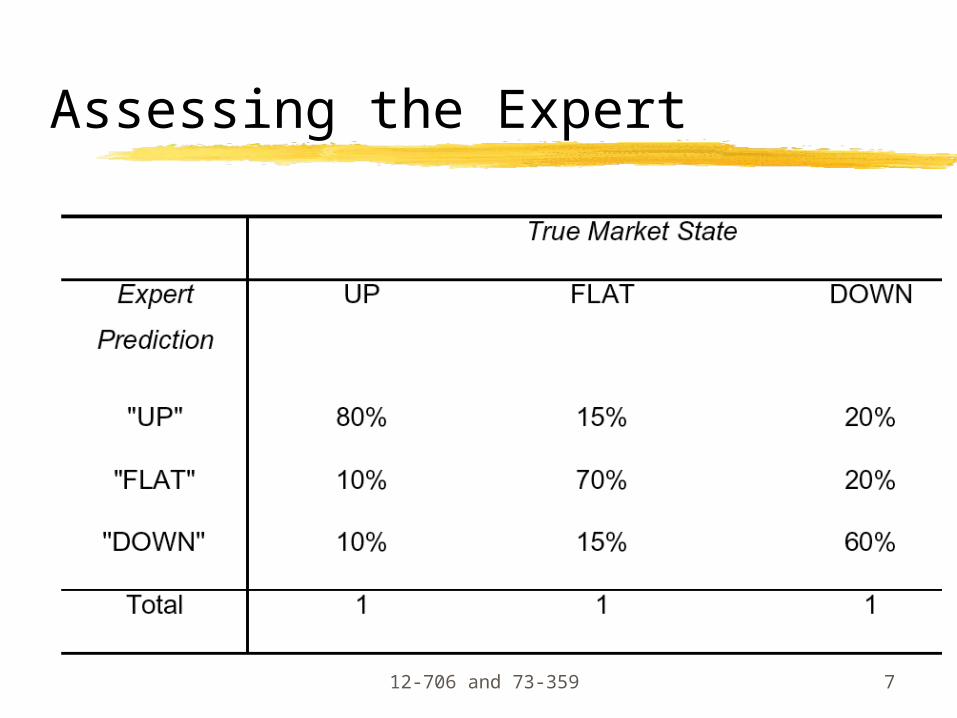
Example: expert admits not always right Use conditional probability (rather than assumption

of 100% correct all the time) to solve trees.

Ideally, they are “almost always right” and “almost never wrong”. In our stock example.. e.g.. P(Up Predicted | Up) is less than but close to 1. P(Up Predicted | Down) is greater than but close to

0

12-706 and 73-359 6

12-706 and 73-359 7

Assessing the Expert

12-706 and 73-359 8

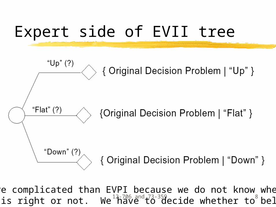
Expert side of EVII tree

This is more complicated than EVPI because we do not know whether the expert is right or not. We have to decide whether to believe her.

12-706 and 73-359 9

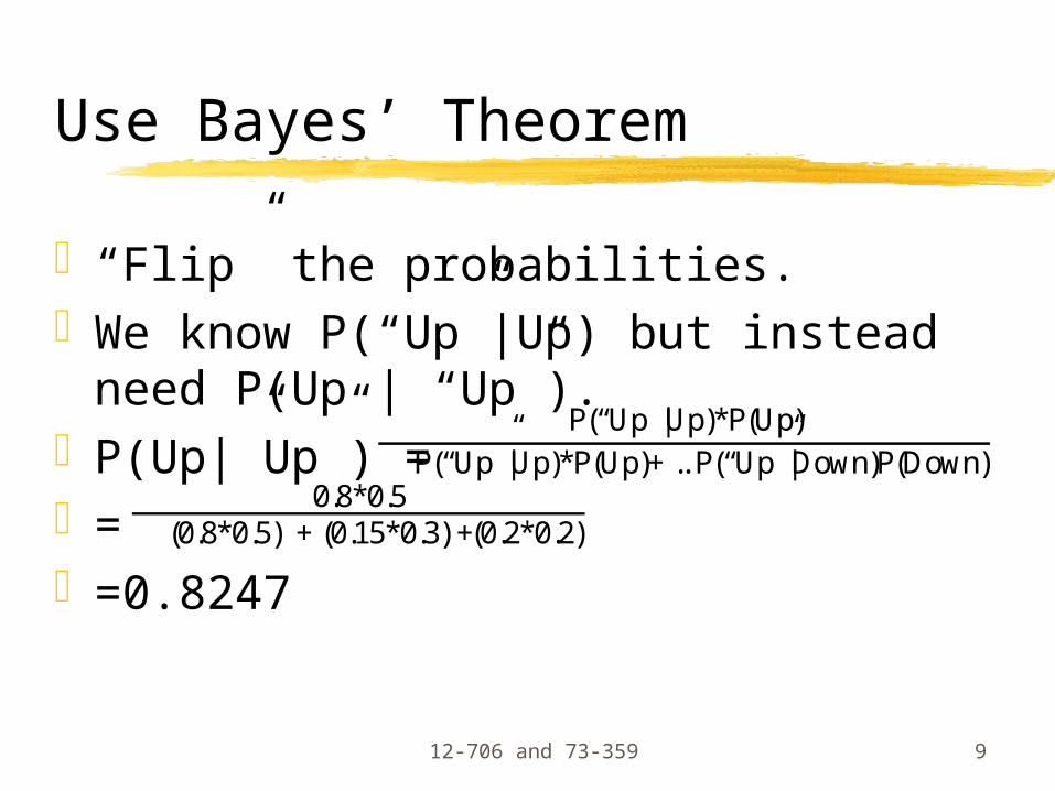
Use Bayes’ Theorem

“Flip” the probabilities.We know P(“Up”|Up) but instead

need P(Up | “Up”).P(Up|”Up”) == =0.8247

P(“Up”|Up)*P(Up)

P(“Up”|Up)*P(Up)+ .. P(“Up”|Down)P(Down)0.8*0.5

(0.8*0.5) + (0.15*0.3) +(0.2*0.2)

12-706 and 73-359 10

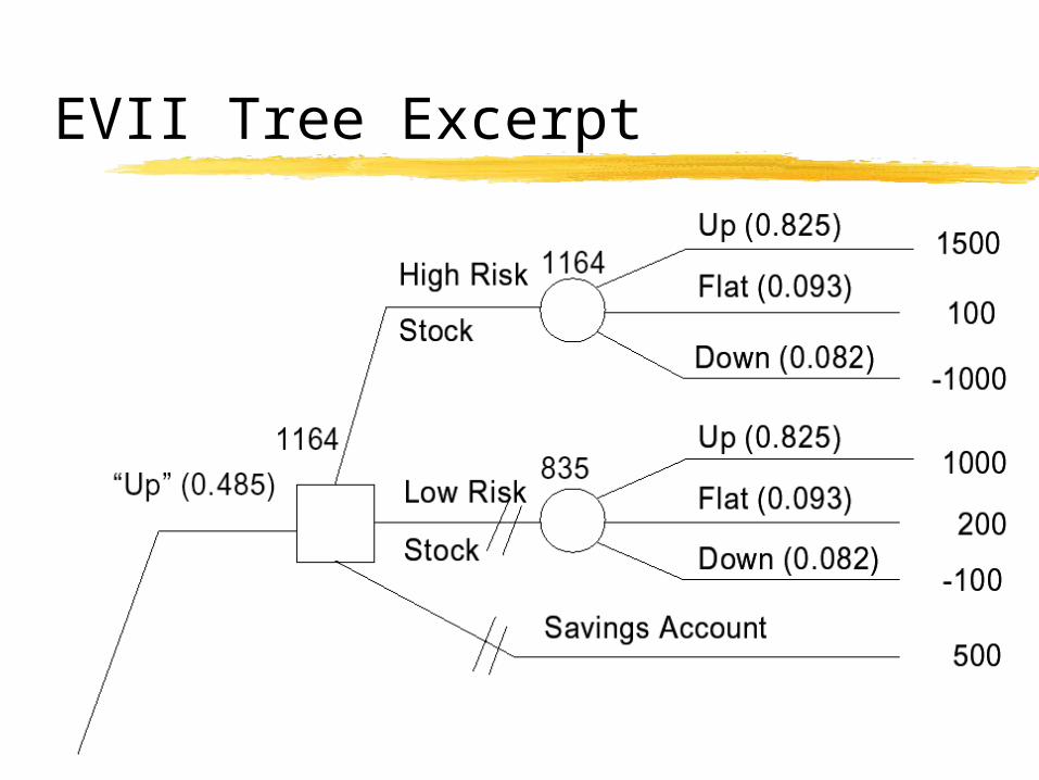
EVII Tree Excerpt

12-706 and 73-359 11

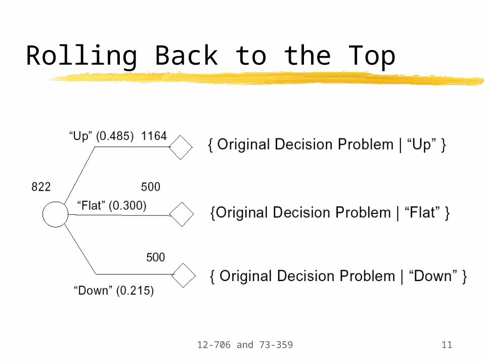
Rolling Back to the Top

12-706 and 73-359 12

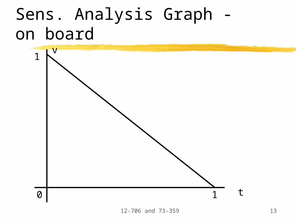
Sens. Analysis for Decision Trees (see Clemen p.189)

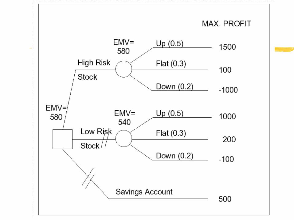
Back to “original stock problem” 3 alternatives.. Interesting results visually

Probabilities: market up, down, samet = Pr(market up), v = P(same)

Thus P(down) = 1 - t - v (must sum to 1!) Or, (t+v must be less than, equal to 1) Know we have a line on our graph

12-706 and 73-359 13

Sens. Analysis Graph - on board

t

v1

0 1

14

12-706 and 73-359 15

Risk Attitudes (Clemen 13)

Our discussions and exercises have focused on EMV (and assume expected-value maximizing decision makers) Not always the case. Some people love the thrill of making tough decisions

regardless of the outcome (not me)

A major problem with Expected Value analysis is that it assumes long-term frequency (i.e., over “many plays of the game”)

12-706 and 73-359 16

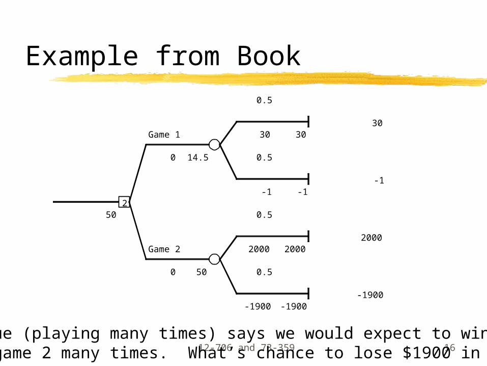
Example from Book0.5

30Game 1 30 30

0 14.5 0.5

-1-1 -1

250 0.5

2000Game 2 2000 2000

0 50 0.5

-1900-1900 -1900

Exp. value (playing many times) says we would expect to win $50 by playing game 2 many times. What’s chance to lose $1900 in Game 2?

12-706 and 73-359 17

Utility Functions

We might care about utility function for wealth (earning money). Are typically: Upward sloping - want more. Concave (opens downward) - preferences for

wealth are limited by your concern for risk. Not constant across all decisions!

Risk-neutral (what is relation to EMV?)Risk-averseRisk-seeking

12-706 and 73-359 18

Individuals

May be risk-neutral across a (limited) range of monetary values But risk-seeking/averse more broadly

May be generally risk averse, but risk-seeking to play the lottery Cost $1, expected value much less than $1

Decision makers might be risk averse at home but risk-seeking in Las Vegas

Such people are dangerous and should be treated with extreme caution. If you see them, notify the authorities.

12-706 and 73-359 19

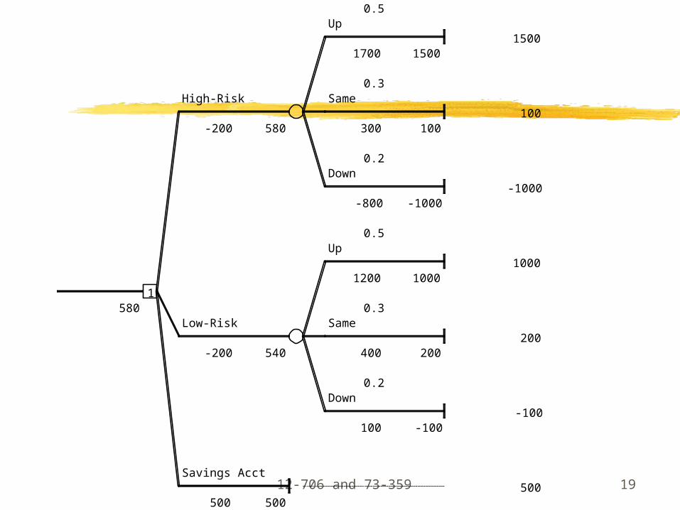
0.5Up

15001700 1500

0.3High-Risk Same

100-200 580 300 100

0.2Down

-1000-800 -1000

0.5Up

10001200 1000

1580 0.3

Low-Risk Same200

-200 540 400 200

0.2Down

-100100 -100

Savings Acct500

500 500

12-706 and 73-359 20

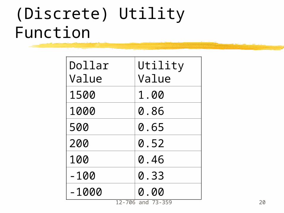
(Discrete) Utility Function

Dollar Value

Utility Value

1500 1.00

1000 0.86

500 0.65

200 0.52

100 0.46

-100 0.33

-1000 0.00

12-706 and 73-359 21

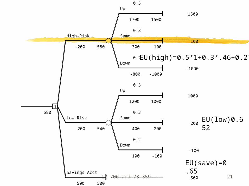
0.5Up

15001700 1500

0.3High-Risk Same

100-200 580 300 100

0.2Down

-1000-800 -1000

0.5Up

10001200 1000

1580 0.3

Low-Risk Same200

-200 540 400 200

0.2Down

-100100 -100

Savings Acct500

500 500

EU(high)=0.5*1+0.3*.46+0.2*0 = 0.64

EU(low)0.652

EU(save)=0.65

12-706 and 73-359 22

Certainty Equivalent (CE)

Amount of money you would trade equally in exchange for an uncertain lottery

What can we infer in terms of CE about our stock investor? EU(low-risk) - his most preferred option maps

to what on his utility function? Thus his CE must be what?

EU(high-risk) -> what is his CE? We could use CE to rank his decision orders

and get the exact same results.

12-706 and 73-359 23

Risk Premium

Is difference between EMV and CE. The risk premium is the amount you are

willing to pay to avoid the risk (like an opportunity cost).

Risk averse: Risk Premium >0 Risk-seeking: Premium <0 (would have

to pay them to give it up!) Risk-neutral: = 0.

12-706 and 73-359 24

Utility Function Assessment

Basically, requires comparison of lotteries with risk-less payoffs

Different people -> different risk attitudes -> willing to accept different level of risk.

Is a matter of subjective judgment, just like assessing subjective probability.

12-706 and 73-359 25

Utility Function Assessment

Two utility-Assessment approaches: Assessment using Certainty Equivalents

Requires the decision maker to assess several certainty equivalents

Assessment using Probabilities This approach use the probability-equivalent (PE) for assessment

technique

Exponential Utility Function: U(x) = 1-e-x/R

R is called risk tolerance

12-706 and 73-359 26

Discussion on Economic Impacts

12-706 and 73-359 27

Summary: Thoughts for Project

Don’t forget we will use the “writing rubric” for grading (see syllabus) 35% of your project grade

Don’t just answer the questions - write a report.

28

Next time:

Deal or No Dealhttp://www.nbc.com/Deal_or_No_Deal/game/