1

Chapter 7

Technology and Production

1

2

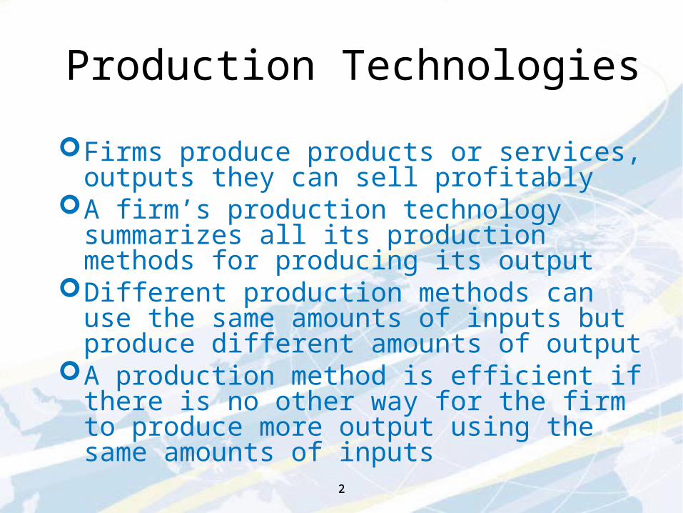
Production Technologies

Firms produce products or services, outputs they can sell profitably

A firm’s production technology summarizes all its production methods for producing its output

Different production methods can use the same amounts of inputs but produce different amounts of output

A production method is efficient if there is no other way for the firm to produce more output using the same amounts of inputs

2

3

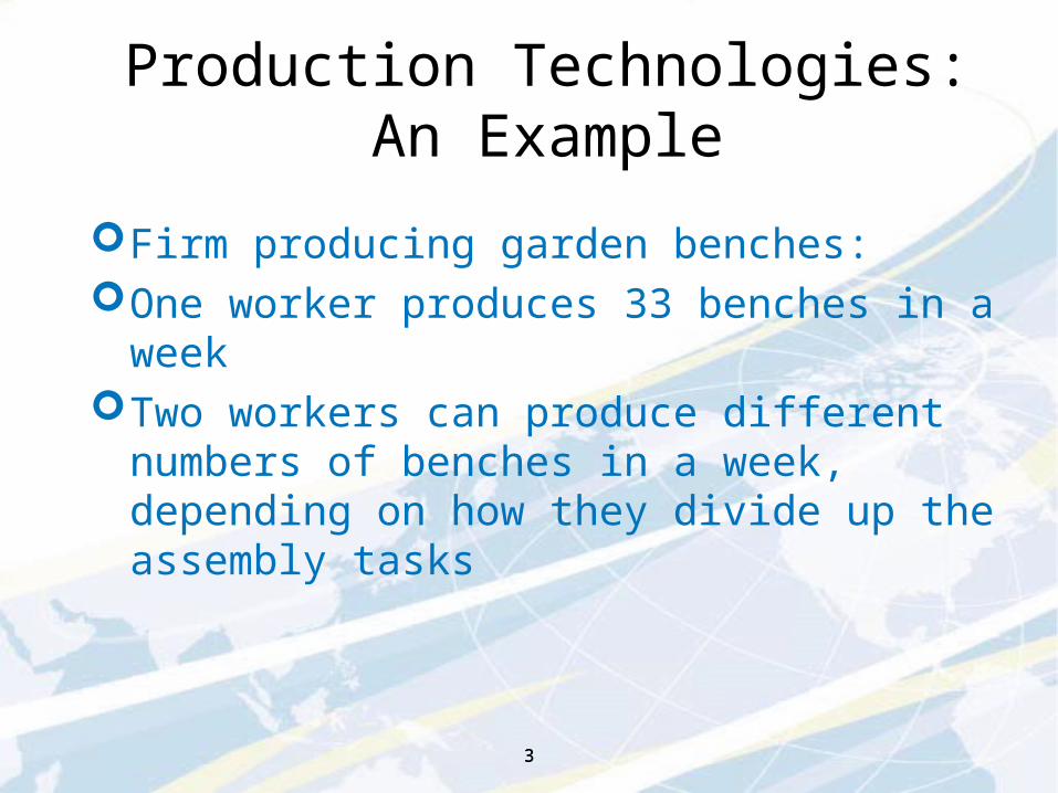
Production Technologies:An Example

Firm producing garden benches:One worker produces 33 benches in a weekTwo workers can produce different numbers of

benches in a week, depending on how they divide up the assembly tasks

3

4

Production Technologies: An Example

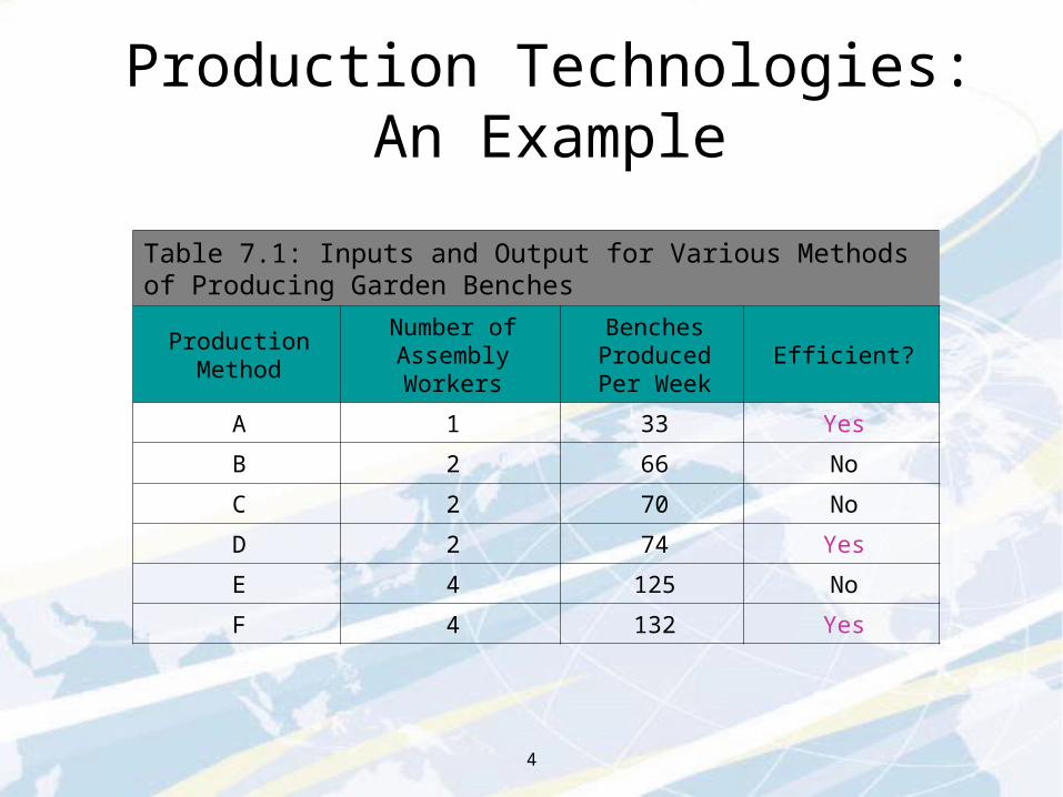
Table 7.1: Inputs and Output for Various Methods of Producing Garden Benches

Production Method

Number of Assembly Workers

Benches Produced Per

WeekEfficient?

A 1 33 Yes

B 2 66 No

C 2 70 No

D 2 74 Yes

E 4 125 No

F 4 132 Yes

5

Production Possibilities Set

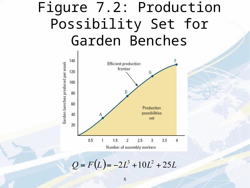
A production possibilities set contains all combinations of inputs and outputs that are possible given the firm’s technology

A firm’s efficient production frontier shows the input-output combinations from all of its efficient production methodsCorresponds to the highest point in the production

possibilities set on the vertical line at a given input level

5

6

Figure 7.2: Production Possibility Set for Garden Benches

7

Production Function

Mathematically, describe efficient production frontier with a production functionOutput=F(Inputs)

Example: Q=F(L)=10LQ is quantity of output, L is quantity of laborSubstitute different amounts of L to see how output

changes as the firm hires different amounts of laborAmount of output never falls when the amount

of input increases Production function shows output produced for

efficient production methods

7

8

Short and Long-Run Production

An input is fixed if it cannot be adjusted over any given time period; it is variable if it can be

Short run: a stage where one or more inputs is fixed

Long run: a stage where all inputs are variable

production process not time Auto manufacturer may need years to build a new

production facility but software firm may need only a month or two to rent and move into a new space

8

9

Average and Marginal Products

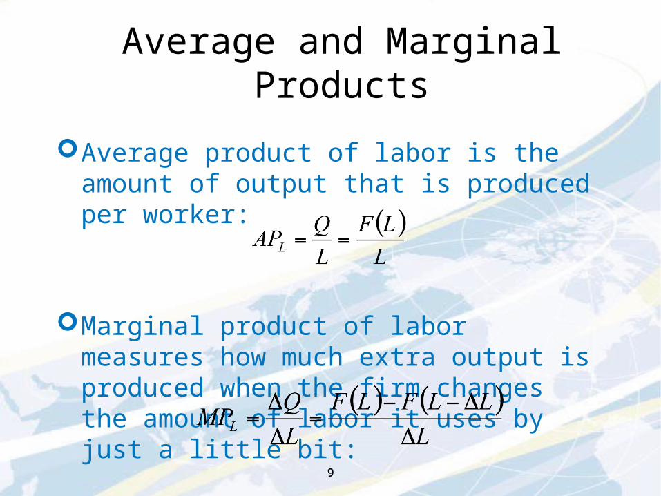
Average product of labor is the amount of output that is produced per worker:

Marginal product of labor measures how much extra output is produced when the firm changes the amount of labor it uses by just a little bit:

9

10

Diminishing Marginal Returns

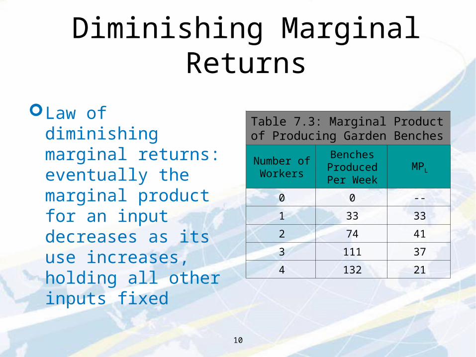
Law of diminishing marginal returns: eventually the marginal product for an input decreases as its use increases, holding all other inputs fixed

Table 7.3: Marginal Product of Producing Garden Benches

Number of Workers

Benches Produced Per Week

MPL

0 0 --

1 33 33

2 74 41

3 111 37

4 132 21

11

Relationship Between AP and MP

Compare MP to AP to see whether AP rises or falls as more of an input is added

MPL shows how much output the marginal worker addsIf he is more productive than average, he brings the

average upIf he is less productive than average, he drives the

average down

11

12

AP and MP Curves

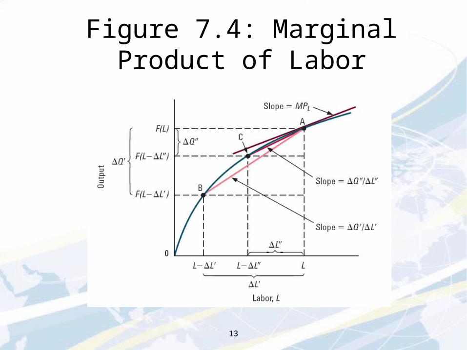
For any point on a short run production function:AP is the slope of the straight line

connecting the point to the originMP equals the slope of the line tangent to

the production function at that point

12

13

Figure 7.4: Marginal Product of Labor

14

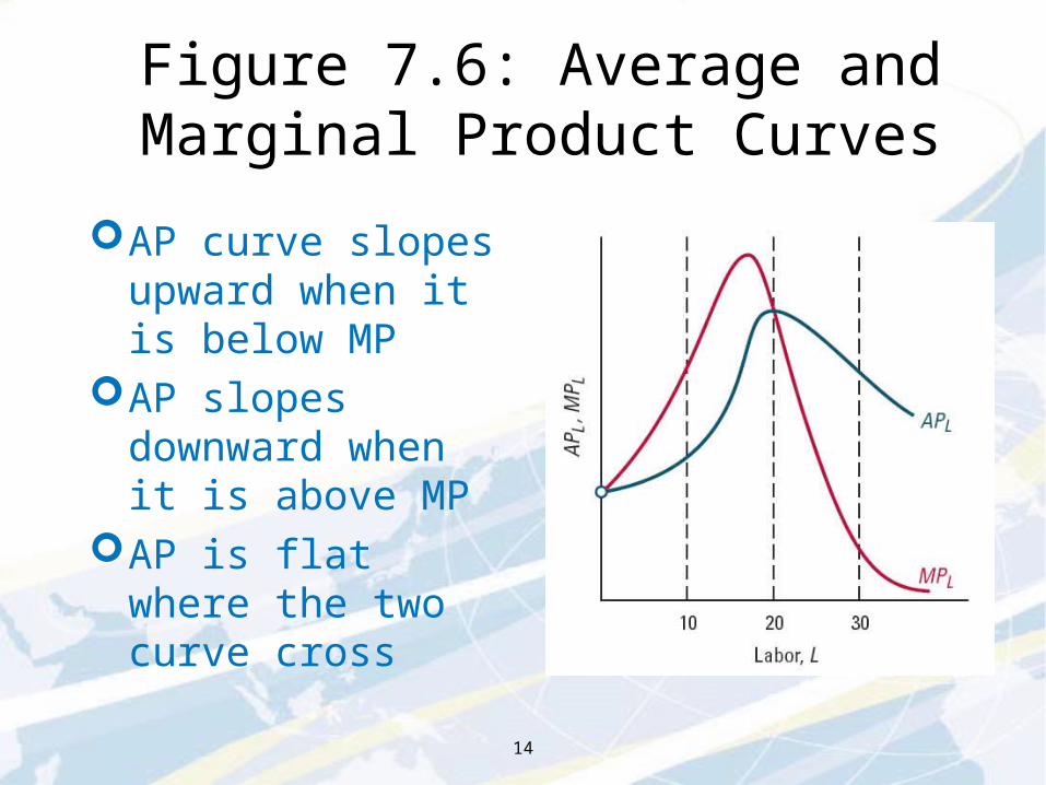
Figure 7.6: Average and Marginal Product Curves

AP curve slopes upward when it is below MP

AP slopes downward when it is above MP

AP is flat where the two curve cross

15

Production with Two Variable Inputs

Most production processes use many variable inputs: labor, capital, materials, and land

Consider a firm that uses two inputs in the long run:Labor (L) and capital (K)Each of these inputs is homogeneousFirm’s production function is Q = F(L,K)

15

16

Production with Two Variable Inputs

When a firm has more than one variable input it can produce a given amount of output with many different combinations of inputsE.g., by substituting K for L

Productive Inputs Principle: Increasing the amounts of all inputs strictly increases the amount of output the firm can produce

16

17

Isoquants

An isoquant identifies all input combinations that efficiently produce a given level of output

Firm’s family of isoquants consists of the isoquants for all of its possible output levels

17

18

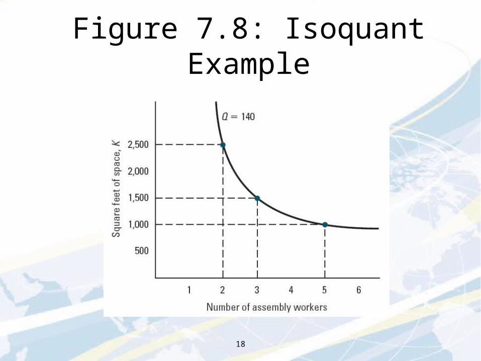
Figure 7.8: Isoquant Example

19

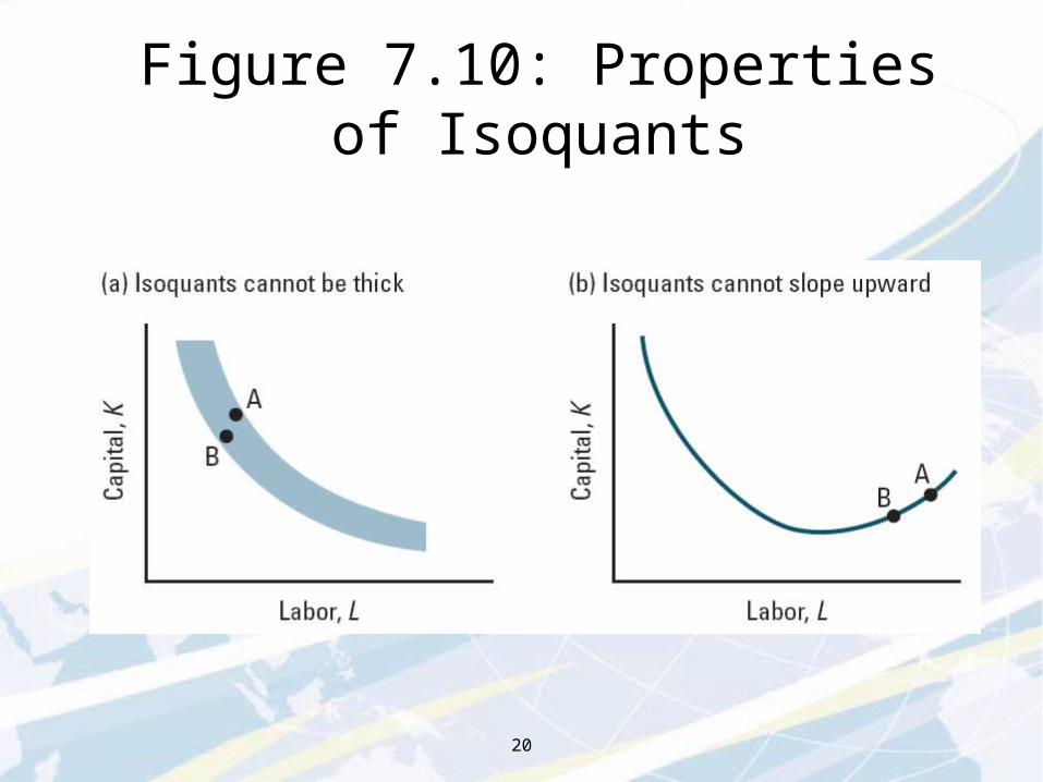
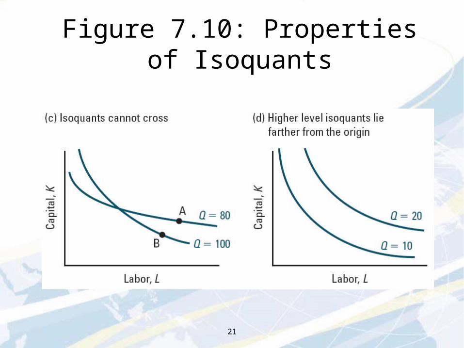
Properties of Isoquants

Isoquants are thinDo not slope upwardThe boundary between input

combinations that produce more and less than a given amount of output

Isoquants from the same technology do not cross

Higher-level isoquants lie farther from the origin

19

20

Figure 7.10: Properties of Isoquants

21

Figure 7.10: Properties of Isoquants

22

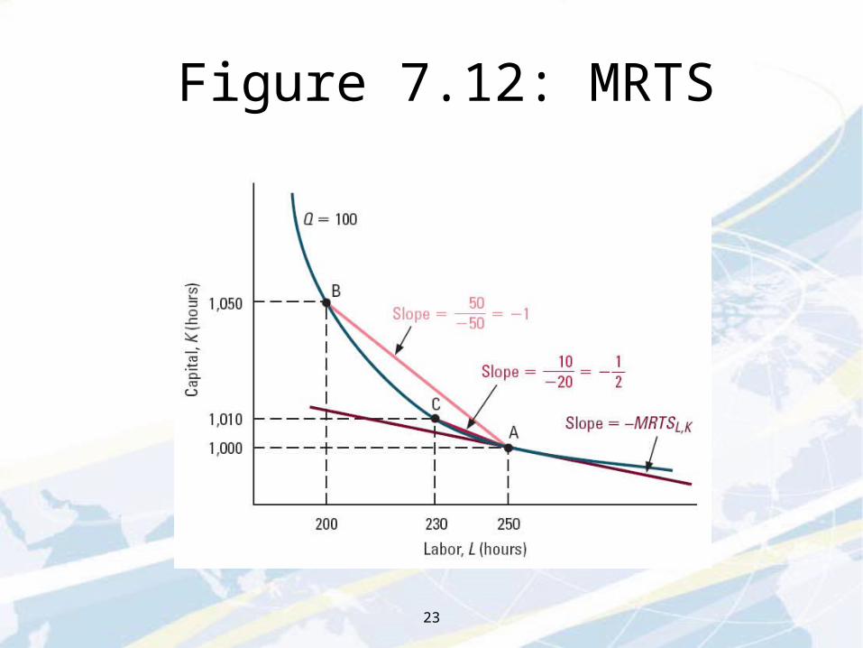
Substitution Between Inputs

Rate that one input can be substituted for another is an important factor for managers in choosing best mix of inputs

Shape of isoquant captures information about input substitution Points on an isoquant have same output but different input mix Rate of substitution for labor with capital is equal to negative

the slope

Marginal Rate of Technical Substitution for input X with input Y: the rate as which a firm must replace units of X with units of Y to keep output unchanged starting at a given input combination

22

23

Figure 7.12: MRTS

24

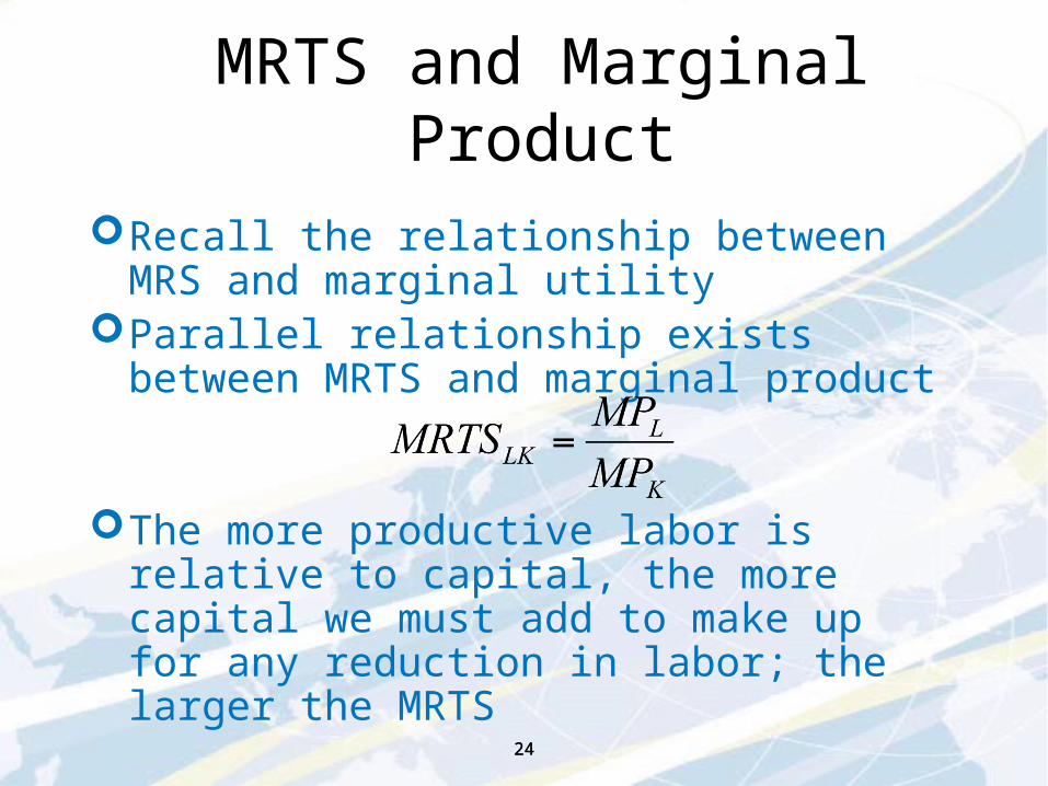
MRTS and Marginal Product

Recall the relationship between MRS and marginal utility

Parallel relationship exists between MRTS and marginal product

The more productive labor is relative to capital, the more capital we must add to make up for any reduction in labor; the larger the MRTS

24

25

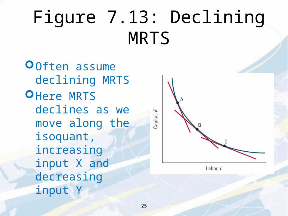
Figure 7.13: Declining MRTS

Often assume declining MRTS

Here MRTS declines as we move along the isoquant, increasing input X and decreasing input Y

26

Extreme Production Technologies

Two inputs are perfect substitutes if their functions are identicalFirm is able to exchange one for another at a fixed

rateEach isoquant is a straight line, constant MRTS

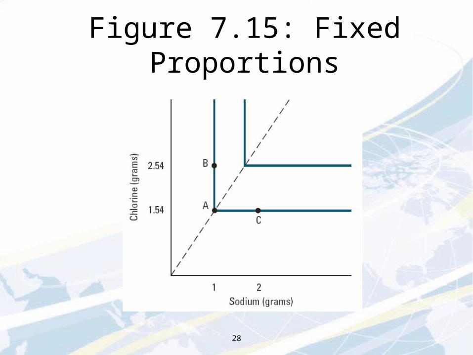
Two inputs are perfect complements whenThey must be used in fixed proportionsIsoquants are L-shaped

26

27

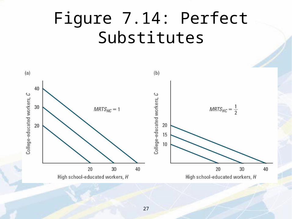
Figure 7.14: Perfect Substitutes

28

Figure 7.15: Fixed Proportions

29

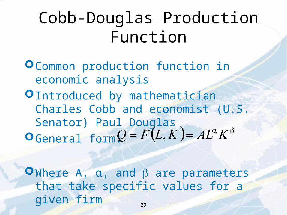
Cobb-Douglas Production Function

Common production function in economic analysis

Introduced by mathematician Charles Cobb and economist (U.S. Senator) Paul Douglas

General form:

Where A, α, and are parameters that take specific values for a given firm

29

30

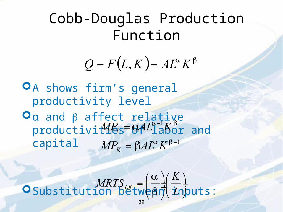
Cobb-Douglas Production Function

A shows firm’s general productivity levelα and affect relative productivities of labor

and capital

Substitution between inputs:

30

31

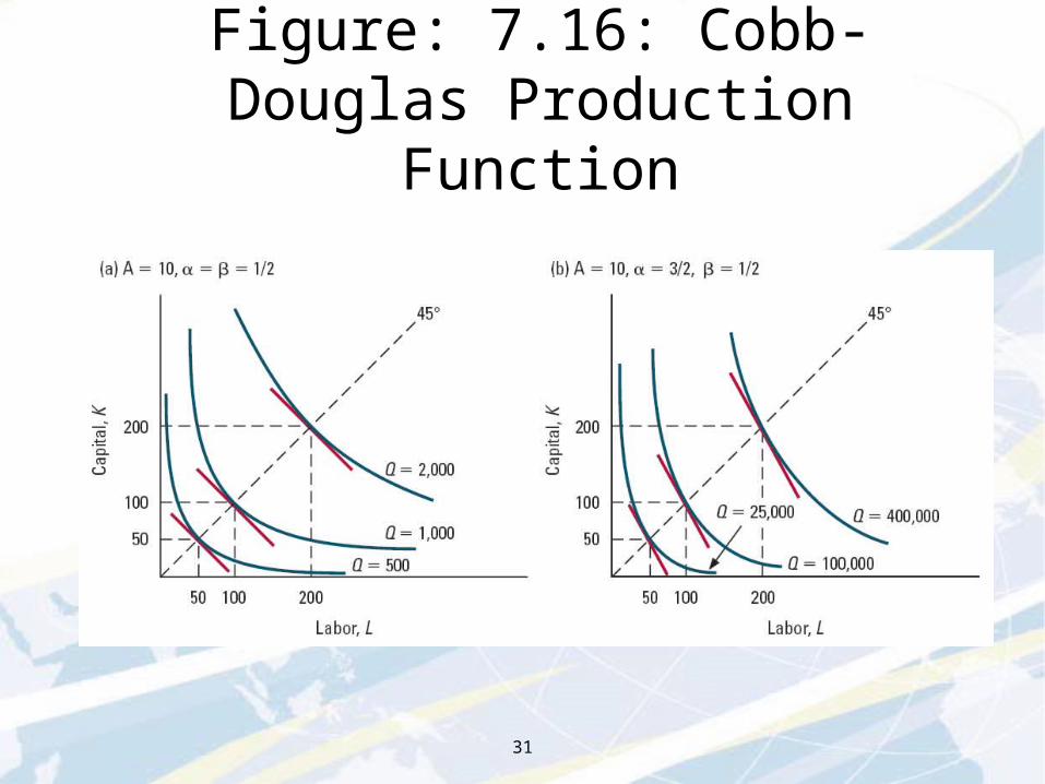
Figure: 7.16: Cobb-Douglas Production Function

32

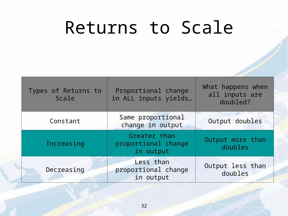
Returns to Scale

Types of Returns to Scale

Proportional change in ALL inputs yields…

What happens when all inputs are doubled?

ConstantSame proportional change in

outputOutput doubles

IncreasingGreater than proportional

change in outputOutput more than

doubles

DecreasingLess than proportional

change in outputOutput less than doubles

33

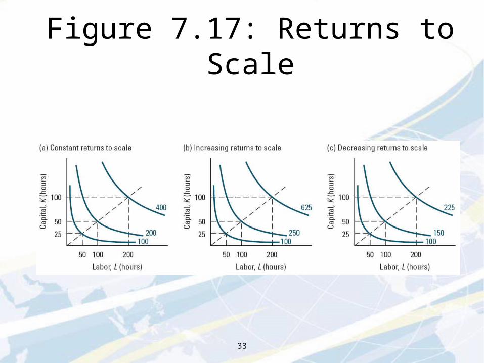
Figure 7.17: Returns to Scale

34

Productivity Differences and Technological Change

A firm is more productive or has higher productivity when it can produce more output use the same amount of inputsIts production function shifts upward at each

combination of inputsMay be either general change in productivity

of specifically linked to use of one inputProductivity improvement that leaves

MRTS unchanged is factor-neutral34