1

Chapter 6

DEMAND RELATIONSHIPS AMONG GOODS

2

The Two-Good Case

• The types of relationships that can occur when there are only two goods are limited

• But this case can be illustrated with two-dimensional graphs

3

Gross Complements

Quantity of x

Quantity of y

x1x0

y1

y0

U1

U0

When the price of y falls, the substitution effect may be so small that the consumer purchases more x and more y

In this case, we call x and y gross complements

x/py < 0

4

Gross Substitutes

Quantity of x

Quantity of y

In this case, we call x and y gross substitutes

x1 x0

y1

y0

U0

When the price of y falls, the substitution effect may be so large that the consumer purchases less x and more y

U1

x/py > 0

5

A Mathematical Treatment• The change in x caused by changes in py

can be shown by a Slutsky-type equation

I

xy

p

x

p

x

Uyy

constant

substitutioneffect (+)

income effect(-) if x is normal

combined effect(ambiguous)

6

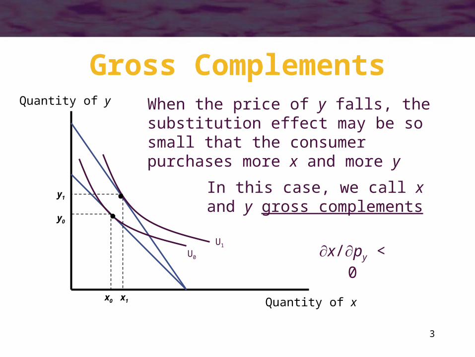
Substitutes and Complements• For the case of many goods, we can

generalize the Slutsky analysis

I

ij

Uj

i

j

i xx

p

x

p

x

constant

for any i or j– this implies that the change in the price of

any good induces income and substitution effects that may change the quantity of every good demanded

7

Substitutes and Complements• Two goods are substitutes if one good

may replace the other in use– examples: tea & coffee, butter & margarine

• Two goods are complements if they are used together– examples: coffee & cream, fish & chips

8

Gross Substitutes and Complements

• The concepts of gross substitutes and complements include both substitution and income effects– two goods are gross substitutes if

xi /pj > 0

– two goods are gross complements if

xi /pj < 0

9

Asymmetry of the Gross Definitions

• One undesirable characteristic of the gross definitions of substitutes and complements is that they are not symmetric

• It is possible for x1 to be a substitute for x2 and at the same time for x2 to be a complement of x1

10

Asymmetry of the Gross Definitions

• Suppose that the utility function for two goods is given by

U(x,y) = ln x + y

• Setting up the Lagrangian

L = ln x + y + (I – pxx – pyy)

11

Asymmetry of the Gross Definitions

gives us the following first-order conditions:

L/x = 1/x - px = 0

L/y = 1 - py = 0

L/ = I - pxx - pyy = 0

• Manipulating the first two equations, we get

pxx = py

12

Asymmetry of the Gross Definitions

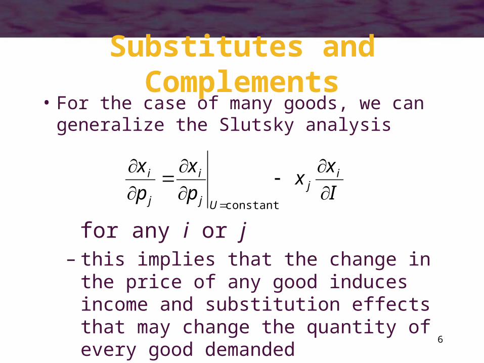
• Inserting this into the budget constraint, we can find the Marshallian demand for y

pyy = I – py

– an increase in py causes a decline in spending on y

• since px and I are unchanged, spending on x must rise ( x and y are gross substitutes)

• but spending on y is independent of px ( x and y are independent of one another)

13

Net Substitutes and Complements

• The concepts of net substitutes and complements focuses solely on substitution effects– two goods are net substitutes if

0constant

Uj

i

p

x

0constant

Uj

i

p

x

– two goods are net complements if

14

Net Substitutes and Complements

• This definition looks only at the shape of the indifference curve

• This definition is unambiguous because the definitions are perfectly symmetric

constantconstant

Ui

j

Uj

i

p

x

p

x

15

Gross Complements

Quantity of x

Quantity of y

x1x0

y1

y0

U1

U0

Even though x and y are gross complements, they are net substitutes

Since MRS is diminishing, the own-price substitution effect must be negative so the cross-price substitution effect must be positive

16

Substitutability with Many Goods

• Once the utility-maximizing model is extended to may goods, a wide variety of demand patterns become possible

• According to Hicks’ second law of demand, “most” goods must be substitutes

17

Substitutability with Many Goods

• To prove this, we can start with the compensated demand function

xc(p1,…pn,V)

• Applying Euler’s theorem yields

0...2

21

1

n

ci

n

ci

ci

p

xp

p

xp

p

xp

18

Substitutability with Many Goods

• In elasticity terms, we get

0...21 cin

ci

ci eee

• Since the negativity of the substitution effect implies that eii

c 0, it must be the case that

0ij

cije

19

Composite Commodities• In the most general case, an individual

who consumes n goods will have demand functions that reflect n(n+1)/2 different substitution effects

• It is often convenient to group goods into larger aggregates– examples: food, clothing, “all other goods”

20

Composite Commodity Theorem• Suppose that consumers choose among n

goods

• The demand for x1 will depend on the prices of the other n-1 commodities

• If all of these prices move together, it may make sense to lump them into a single composite commodity (y)

21

Composite Commodity Theorem

• Let p20…pn

0 represent the initial prices of

these other commodities– assume that they all vary together (so that the

relative prices of x2…xn do not change)

• Define the composite commodity y to be total expenditures on x2…xn at the initial

prices

y = p20x2 + p3

0x3 +…+ pn0xn

22

Composite Commodity Theorem• The individual’s budget constraint is

I = p1x1 + p20x2 +…+ pn

0xn = p1x1 + y

• If we assume that all of the prices p20…pn

0

change by the same factor (t > 0) then the budget constraint becomes

I = p1x1 + tp20x2 +…+ tpn

0xn = p1x1 + ty

– changes in p1 or t induce substitution effects

23

Composite Commodity Theorem

• As long as p20…pn

0 move together, we can

confine our examination of demand to choices between buying x1 and “everything

else”

• The theorem makes no prediction about how choices of x2…xn behave

– only focuses on total spending on x2…xn

24

Composite Commodity• A composite commodity is a group of

goods for which all prices move together

• These goods can be treated as a single commodity– the individual behaves as if he is choosing

between other goods and spending on this entire composite group

25

Example: Composite Commodity

• Suppose that an individual receives utility from three goods:– food (x)– housing services (y), measured in

hundreds of square feet– household operations (z), measured by

electricity use

• Assume a CES utility function

26

Example: Composite Commodity

• The Lagrangian technique can be used to derive demand functions

zyxzyxU

111 ),,( utility

zxyxx pppppx

I

zyxyy pppppy

I

yzxzz pppppz

I

27

Example: Composite Commodity

• If initially I = 100, px = 1, py = 4, and pz = 1, then

• x* = 25, y* = 12.5, z* = 25– $25 is spent on food and $75 is spent on

housing-related needs

28

Example: Composite Commodity

• If we assume that the prices of housing services (py) and electricity (pz) move together, we can use their initial prices to define the “composite commodity” housing (h)

h = 4y + 1z

• The initial quantity of housing is the total spent on housing (75)

29

Example: Composite Commodity

• If I = 100, px = 1, py = 4, and ph = 1, then x* = 25 and spending on housing (h*) = 75

hxy pppx

3

I

• Now x can be shown as a function of I, px, and ph

30

Example: Composite Commodity

• If py rises to 16 and pz rises to 4 (with px remaining at 1), ph would also rise to 4

• The demand for x would fall to

7

100

431

100*

x

• Housing purchases would be given by

7

600

7

100100* hPh

31

Example: Composite Commodity

• Since ph = 4, h* = 150/7

• If I = 100, px = 1, py = 16, and pz = 4, the

individual demand functions show that

x* = 100/7, y* = 100/28, z* = 100/14

• This means that the amount of h that is consumed can also be computed as

h* = 4y* + 1z* = 150/7