1

Chapter 3

Market Structure

and

Market Power

2

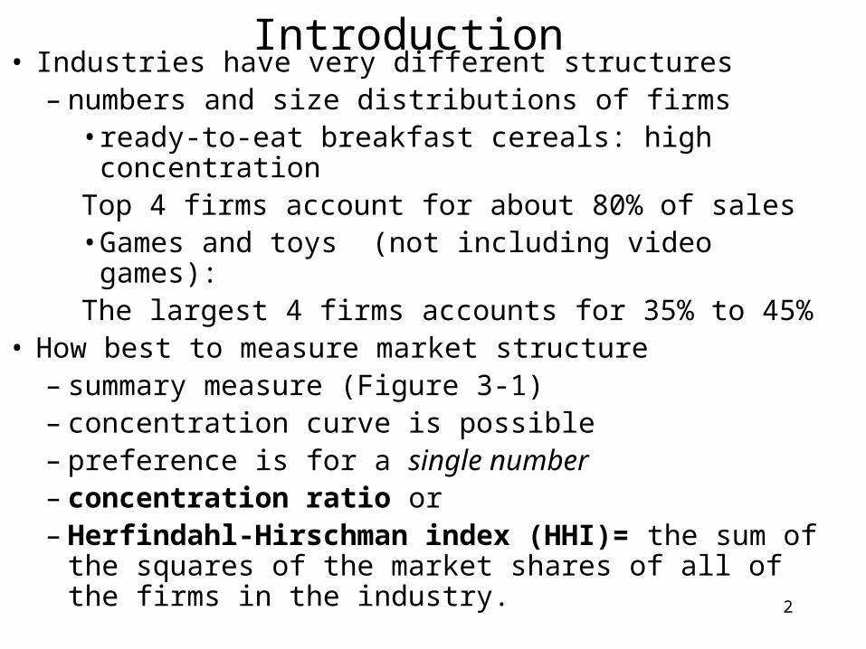
Introduction• Industries have very different structures

– numbers and size distributions of firms• ready-to-eat breakfast cereals: high concentrationTop 4 firms account for about 80% of sales• Games and toys (not including video games): The largest 4 firms accounts for 35% to 45%

• How best to measure market structure– summary measure (Figure 3-1)– concentration curve is possible– preference is for a single number– concentration ratio or – Herfindahl-Hirschman index (HHI)= the sum of the

squares of the market shares of all of the firms in the industry.

3

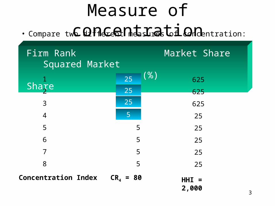
Measure of concentration• Compare two different measures of concentration:

Firm Rank Market Share Squared Market (%) Share

1 25

2 25

3 25

4 5

5 5

6 5

7 5

8 5

625

625

625

25

25

25

25

25

CR4 = 80Concentration Index HHI = 2,000

25

25

25

5

4

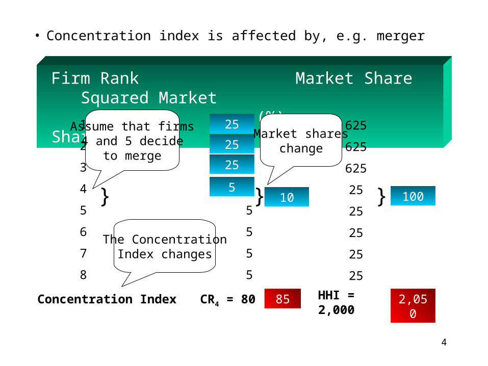
• Concentration index is affected by, e.g. merger

Firm Rank Market Share Squared Market (%) Share

1 25

2 25

3 25

4 5

5 5

6 5

7 5

8 5

625

625

625

25

25

25

25

25

CR4 = 80Concentration Index HHI = 2,000

25

25

25

5} } }10

85

100

2,050

Assume that firms4 and 5 decide

to merge

The ConcentrationIndex changes

Market shareschange

5

3.1.1 What is a market?• No clear consensus:To use CR4 or HHI as an

overall measure of a market’s structure, we need to be able to identify a well-defined market first.Example 1, the market for automobiles

• should we include light trucks; pick-ups SUVs?Example 2, the market for soft drinks

• what are the competitors for Coca Cola and Pepsi?– With whom do McDonalds and Burger King

compete?• Presumably define a market by closeness in

substitutability of the commodities involved– how close is close?

6

Market definition (cont.)– how homogeneous do commodities have to be?

• Does wood compete with plastic? Rayon with wool?

• Definition is important– without consistency concept of a market is meaningless– need indication of competitiveness of a market: affected by

definition– public policy: decisions on mergers can turn on market

definition• Staples/Office Depot merger rejected on market definition• Coca Cola expansion turned on market definition

• Standard approach has some consistency– based upon industrial data– substitutability is production not consumption (ease of data

collection)

7

• Government statistical sourcesCensus Bureau:

Standard Industrial Classification (SIC)North American Industry Classification System

(NAICS)• The measure of concentration varies across countries• Use of production-based statistics has limitations:

– can put in different industries products that are in the same market

• The international dimension is important– Boeing/McDonnell-Douglas merger– relevant market for automobiles, oil, hairdressing

Market definition (cont.)

8

• Geography is important– barrier to entry if the product is expensive to

transport– but customers can move

• what is the relevant market for a beach resort or ski-slope?

• Vertical relations between firms are important– most firms make intermediate rather than final goods– firm has to make a series of make-or-buy choices– upstream and downstream production– measures of concentration may assign firms at

different stages to the same industry• do vertical relations affect underlying structure?

Market definition (cont.)

9

– Firms at different stages may also be assigned to different industries

• bottlers of soft drinks: low concentration

• suppliers of sift drinks: high concentration

• the bottling sector is probably not competitive.

• In sum: market definition poses real problems

– existing methods represent a reasonable compromise

Market definition (cont.)

10

• Measuring Market Power• The Lerner Index (LI) is one way to measure how well a

market performs from an efficiency point of view. The LI measures how far the outcome is from the competitive ideal in the following way:

• LI= (P-MC)/P• Because LI directly reflects the discrepancy between price

and marginal cost it captures much of what we are interested in when it comes to the exercise of market power.

• For a competitive firm, LI is zero since such a firm prices at marginal cost.

• For a pure monopolist, on the other hand, the LI can be shown to be the inverse of the elasticity of demand-the less elastic the demand the greater is the price-marginal cost distortion. To see this, a monopolist’s MR = P+(dp/dQ)*Q

• For profit maximization: MR=MC

11

• So, P + (dP/dQ)*Q = MC.

• Rearranging and dividing by price P, we obtain (P-MC)/P = - (dP/dQ)*(Q/P) = 1/ elasticity of the demand.

• Note that the LI can never exceed 1 and that it can only achieve this maximum value if MC=0.

• With more than one but not “many” firms, the Lerner Index is more complicated: need to average.– suppose the goods are homogeneous so all firms sell at

the same price

LI =P-siMCi

P

12

$/unit

Quantity

AC1

Assume two identical firms each with costs AC1

If they are to produce a given output at lowest cost, they must operate at the same marginal

costMC Why? Assume firm A is operating at MCA and firm B is operating at MCBMCA

MCB

Transferring one unit of output from A to B lowers total costMC´A

MC´B

If the two firms operate at the same marginal cost they must produce identical

outputs

Suppose not: firm A has output QA and firm B has output QB

Transferring one unit of output from A to B lowers total cost

QAQB

13

$/unit

Quantity

AC1 AC2

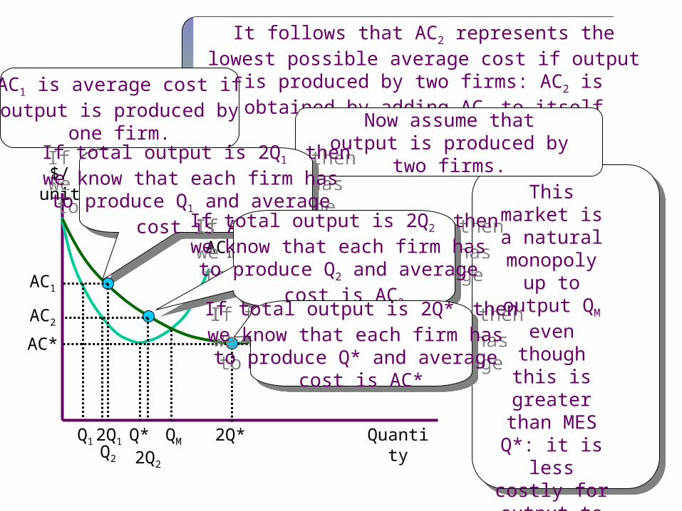
It follows that AC2 represents the lowest possible average cost if output is produced by two firms: AC2 is obtained

by adding AC1 to itself horizontally

This market is a natural

monopoly up to output QM even though this is greater than

MES Q*: it is less costly for output to be produced by

one rather than two firms:

subadditivity

Q* 2Q*QM

AC1 is average cost ifoutput is produced by

one firm.Now assume that

output is produced bytwo firms.If total output is 2Q1 then

we know that each firm has to produce Q1 and average

cost is AC1

If total output is 2Q1 thenwe know that each firm has to produce Q1 and average

cost is AC1

AC1

2Q1Q1

2Q2Q2

If total output is 2Q2 thenwe know that each firm has to produce Q2 and average

cost is AC2

If total output is 2Q2 thenwe know that each firm has to produce Q2 and average

cost is AC2If total output is 2Q* then

we know that each firm has to produce Q* and average

cost is AC*

If total output is 2Q* thenwe know that each firm has to produce Q* and average

cost is AC*

AC2

AC*

14

Chapter 4Technology and Cost

15

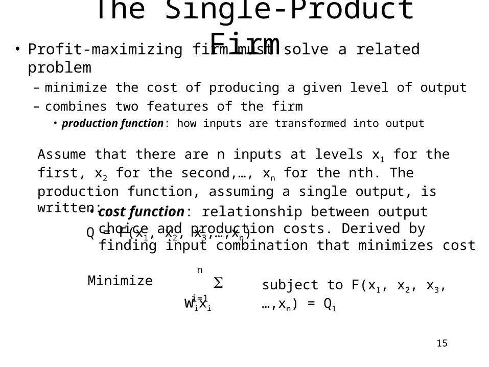
The Single-Product Firm• Profit-maximizing firm must solve a related problem

– minimize the cost of producing a given level of output

– combines two features of the firm• production function: how inputs are transformed into output

Assume that there are n inputs at levels x1 for the first, x2 for the second,…, xn for the nth. The production function, assuming a single output, is written:

Q = F(x1, x2, x3,…,xn)• cost function: relationship between output choice and

production costs. Derived by finding input combination that minimizes cost

Minimize subject to F(x1, x2, x3,…,xn) = Q1 wixi

i=1

n

16

• Review input choice: one output and two inputs

x2

x1

Q0

Q1

Q2

The production functioncan be illustrated as a set of

isoquants, one foreach level of output

The production functioncan be illustrated as a set of

isoquants, one foreach level of output

Production cost can beillustrated as a set of

isocost lines, with slopew1/w2. The lower theisocost line, the lower

the cost.

Production cost can beillustrated as a set of

isocost lines, with slopew1/w2. The lower theisocost line, the lower

the cost.

Cost of producing output Q1 is minimized

by finding the pointwhere an isocost line

is tangent to theQ1 isoquant

Cost of producing output Q1 is minimized

by finding the pointwhere an isocost line

is tangent to theQ1 isoquant

x11

x12

The input choiceis x1

1 of input 1and x1

2 of input 2

The input choiceis x1

1 of input 1and x1

2 of input 2

Now assume that input 1 becomes cheaper

This makes the isocost lines less steep

The new cost-minimizing point

The new cost-minimizing point

More ofinput 1 is

used and lessof input 2

More ofinput 1 is

used and lessof input 2 x2

1

x22

The cost-minimizing input combination changes

The cost-minimizing input combination changes

17

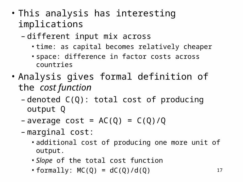
• This analysis has interesting implications– different input mix across

• time: as capital becomes relatively cheaper

• space: difference in factor costs across countries

• Analysis gives formal definition of the cost function– denoted C(Q): total cost of producing output Q– average cost = AC(Q) = C(Q)/Q– marginal cost:

• additional cost of producing one more unit of output.

• Slope of the total cost function

• formally: MC(Q) = dC(Q)/d(Q)

18

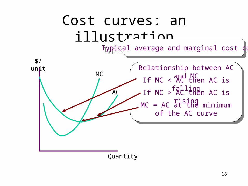
Cost curves: an illustration

$/unit

Quantity

AC

MC

Typical average and marginal cost curvesTypical average and marginal cost curves

Relationship between AC and MC

If MC < AC then AC is falling

If MC > AC then AC is rising

MC = AC at the minimum of the AC curve

19

Economies of scale• Definition: average costs fall with an increase in output• Represented by the scale economy index

S =AC(Q)

MC(Q)• S > 1: economies of scale• S < 1: diseconomies of scale• S is the inverse of the elasticity of cost with respect to output

C =dC(Q)

C(Q)

dQ

Q=

dC(Q)

dQ

C(Q)

Q=

MC(Q)

AC(Q)=

1

S

20

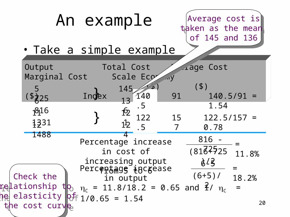
An example

• Take a simple example

Output Total Cost Average Cost Marginal Cost Scale Economy ($) ($) ($) Index5 725 145

6 816 13691}

11 1331 121

12 1488 124} 157

140.5 140.5/91 = 1.54

122.5/157 = 0.78

Average cost istaken as the mean

of 145 and 136

Average cost istaken as the mean

of 145 and 136

122.5

Check the relationship to the elasticity of the cost curve

Check the relationship to the elasticity of the cost curve

816 - 725Percentage increase in cost of increasing output from 5 to 6 (816+725)/2

= 11.8%

Percentage increase in output6-5

(6+5)/2= 18.2%

C = 11.8/18.2 = 0.65 and 1/ C = 1/0.65 = 1.54

21

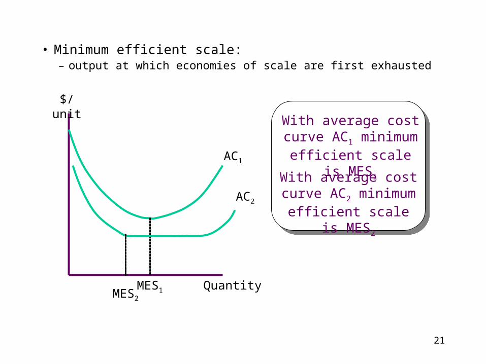
• Minimum efficient scale: – output at which economies of scale are first exhausted

$/unit

Quantity

AC1

MES1

AC2

MES2

With average cost curve AC1 minimum efficient

scale is MES1

With average cost curve AC2 minimum efficient

scale is MES2

22

Natural monopoly• If the extent of the market is less than MES then the market is a

natural monopoly: S > 1 in such a market.• But a natural monopoly can exist even if S < 1.

Economies of scale• Sources of economies of scale

– “the 60% rule”: capacity related to volume while cost is related to surface area

– product specialization and the division of labor– “economies of mass reserves”: economize on inventory,

maintenance, repair– indivisibilities

23

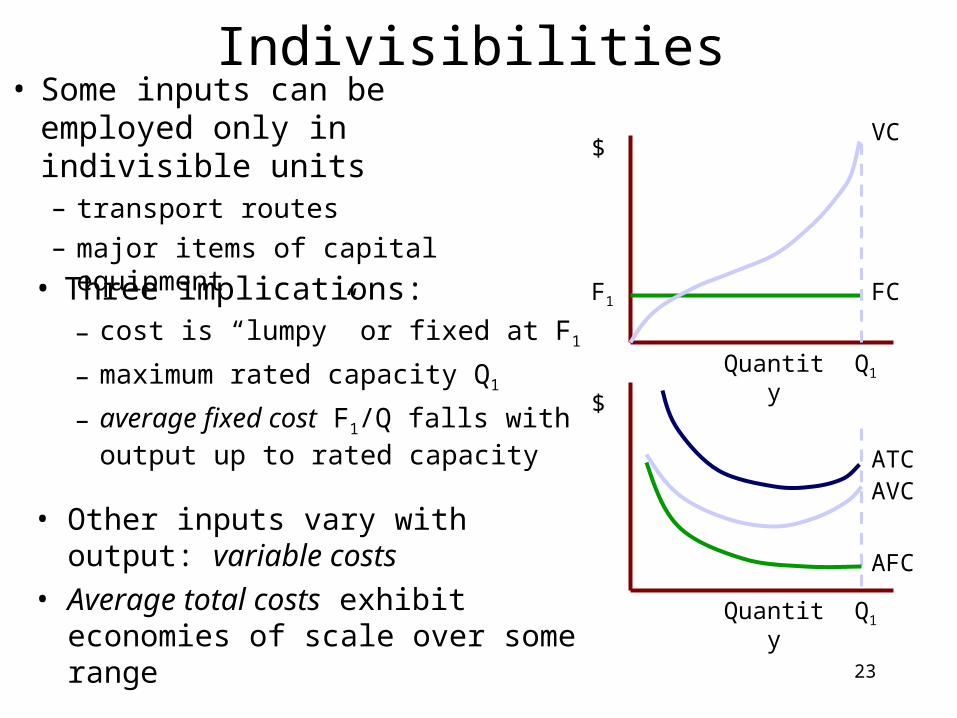
Indivisibilities• Some inputs can be employed

only in indivisible units– transport routes

– major items of capital equipment

$

$

Quantity

Quantity

Q1

Q1

FC

VC

AFC

AVCATC

• Three implications:– cost is “lumpy” or fixed at F1

– maximum rated capacity Q1

– average fixed cost F1/Q falls with output up to rated capacity

• Other inputs vary with output: variable costs

• Average total costs exhibit economies of scale over some range

F1

24

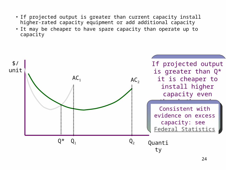
• If projected output is greater than current capacity install higher-rated capacity equipment or add additional capacity

• It may be cheaper to have spare capacity than operate up to capacity

$/unit

AC1 AC2

QuantityQ1 Q2

If projected output is greater than Q* it is cheaper to

install higher capacity even though there is spare

capacity

Q*

Consistent with evidence on excess capacity: see

Federal Statistics

25

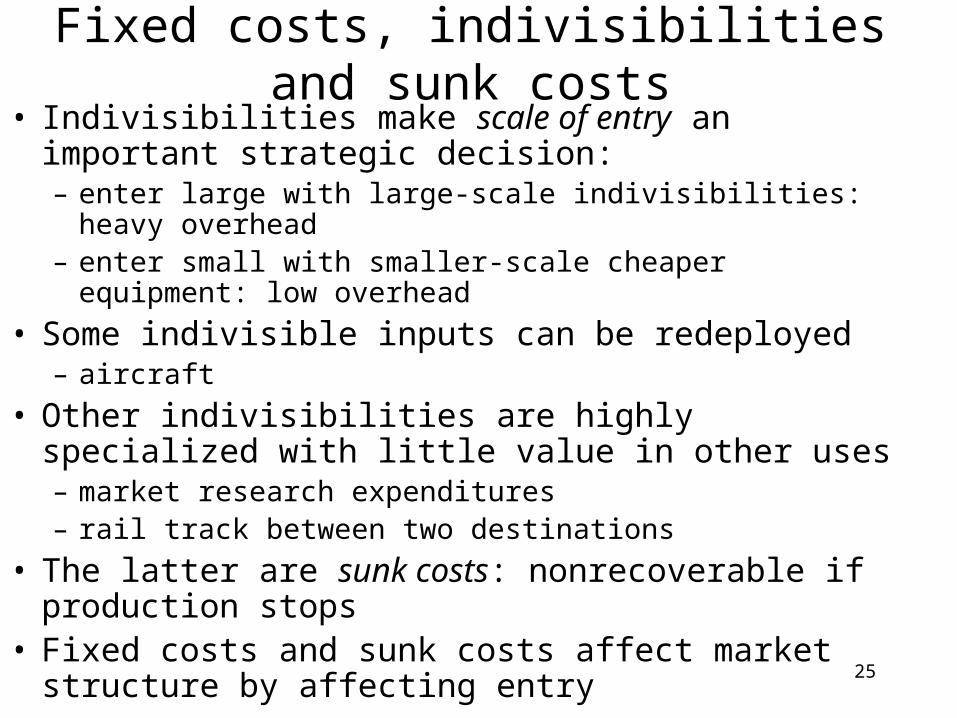
• Indivisibilities make scale of entry an important strategic decision:– enter large with large-scale indivisibilities: heavy overhead– enter small with smaller-scale cheaper equipment: low overhead

• Some indivisible inputs can be redeployed– aircraft

• Other indivisibilities are highly specialized with little value in other uses– market research expenditures– rail track between two destinations

• The latter are sunk costs: nonrecoverable if production stops

• Fixed costs and sunk costs affect market structure by affecting entry

Fixed costs, indivisibilities and sunk costs

26

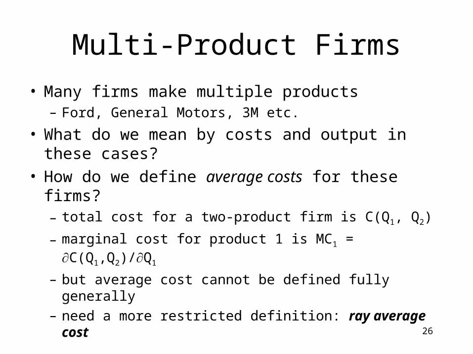
Multi-Product Firms

• Many firms make multiple products– Ford, General Motors, 3M etc.

• What do we mean by costs and output in these cases?• How do we define average costs for these firms?

– total cost for a two-product firm is C(Q1, Q2)

– marginal cost for product 1 is MC1 = C(Q1,Q2)/Q1

– but average cost cannot be defined fully generally

– need a more restricted definition: ray average cost

27

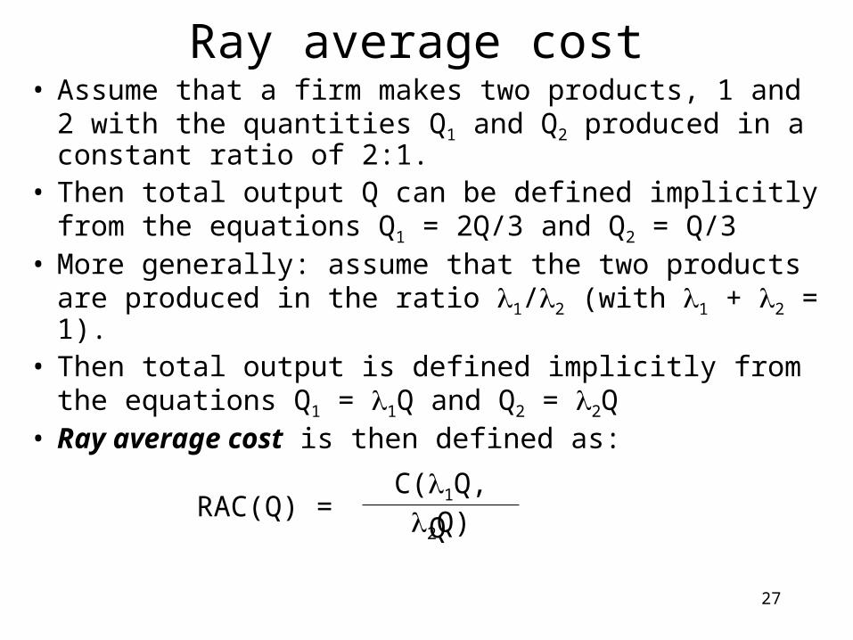
Ray average cost• Assume that a firm makes two products, 1 and 2 with the

quantities Q1 and Q2 produced in a constant ratio of 2:1.• Then total output Q can be defined implicitly from the

equations Q1 = 2Q/3 and Q2 = Q/3• More generally: assume that the two products are

produced in the ratio 1/2 (with 1 + 2 = 1).• Then total output is defined implicitly from the equations

Q1 = 1Q and Q2 = 2Q• Ray average cost is then defined as:

RAC(Q) =C(1Q, 2Q)

Q

28

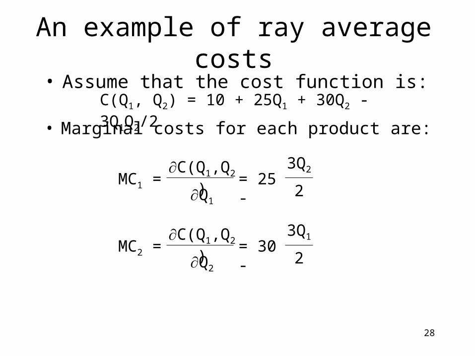
An example of ray average costs

• Marginal costs for each product are:

C(Q1, Q2) = 10 + 25Q1 + 30Q2 - 3Q1Q2/2• Assume that the cost function is:

MC1 =C(Q1,Q2)

Q1

= 25 -3Q2

2

MC2 =C(Q1,Q2)

Q2

= 30 -3Q1

2

29

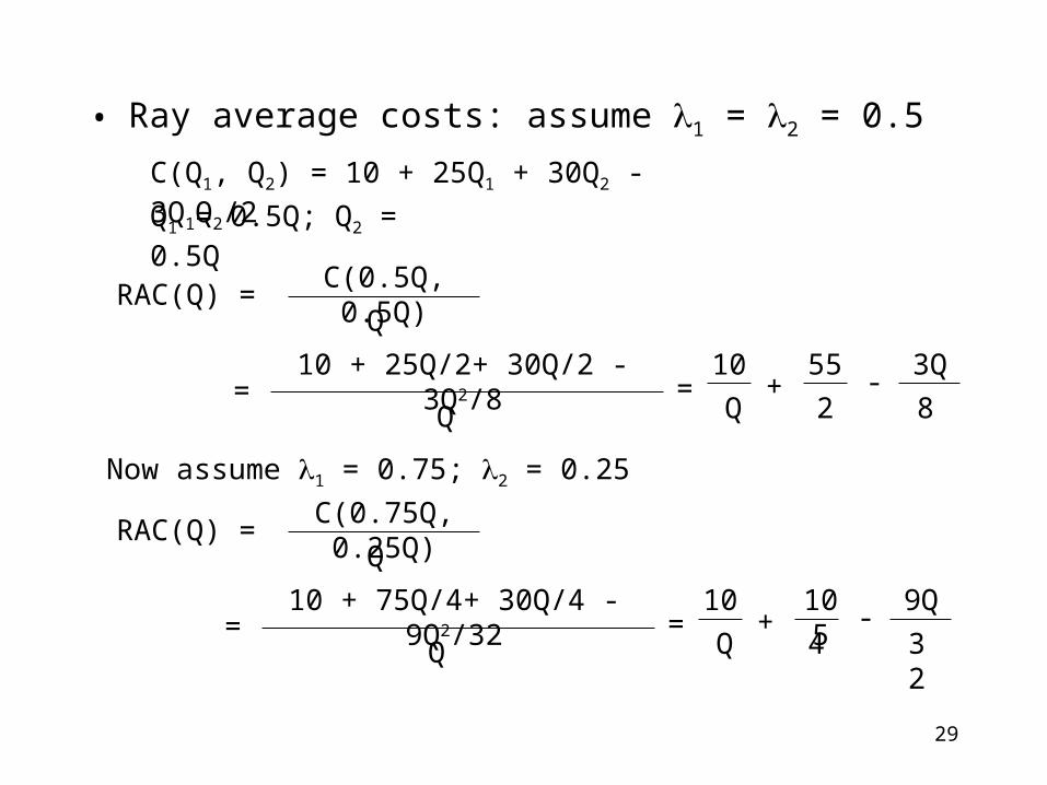
• Ray average costs: assume 1 = 2 = 0.5

C(Q1, Q2) = 10 + 25Q1 + 30Q2 - 3Q1Q2/2

Q1 = 0.5Q; Q2 = 0.5Q

RAC(Q) =C(0.5Q, 0.5Q)

Q

=10 + 25Q/2+ 30Q/2 - 3Q2/8

Q=

10

Q+

55

2-

3Q

8

Now assume 1 = 0.75; 2 = 0.25

RAC(Q) =C(0.75Q, 0.25Q)

Q

=10 + 75Q/4+ 30Q/4 - 9Q2/32

Q=

10

Q+

105

4-

9Q

32

30

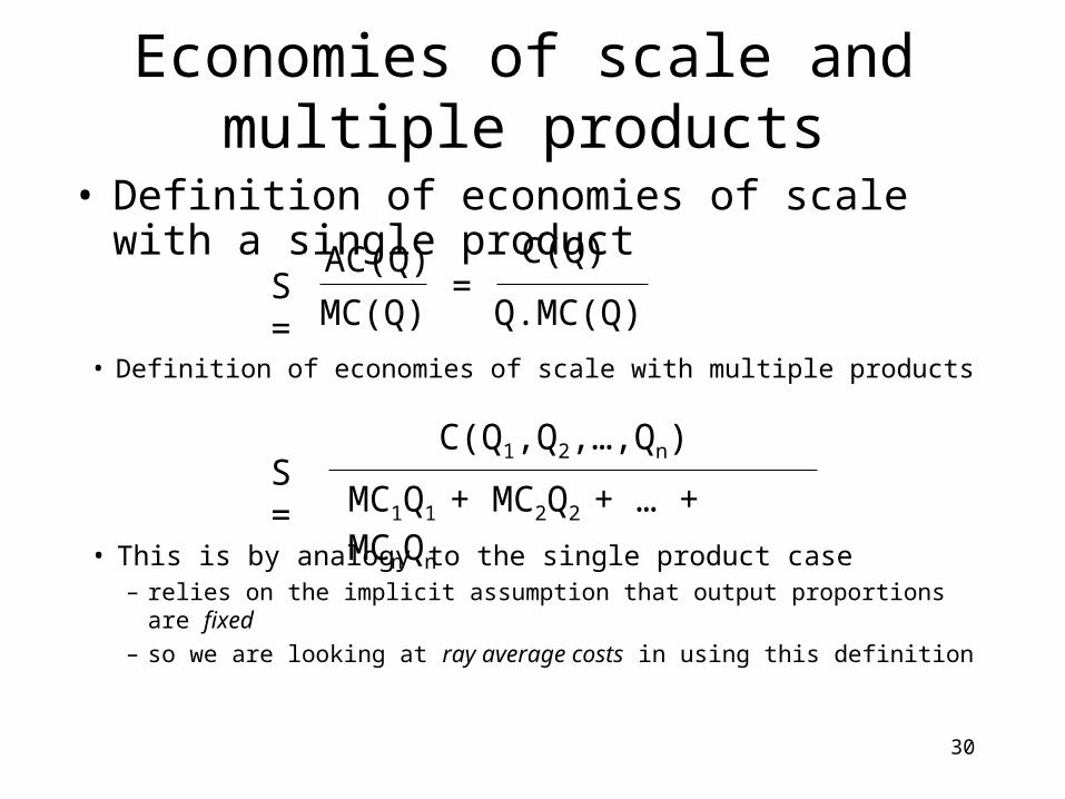
Economies of scale and multiple products

• Definition of economies of scale with a single product

S =AC(Q)

MC(Q)=

C(Q)

Q.MC(Q)

• Definition of economies of scale with multiple products

S =C(Q1,Q2,…,Qn)

MC1Q1 + MC2Q2 + … + MCnQn

• This is by analogy to the single product case– relies on the implicit assumption that output proportions are fixed– so we are looking at ray average costs in using this definition

31

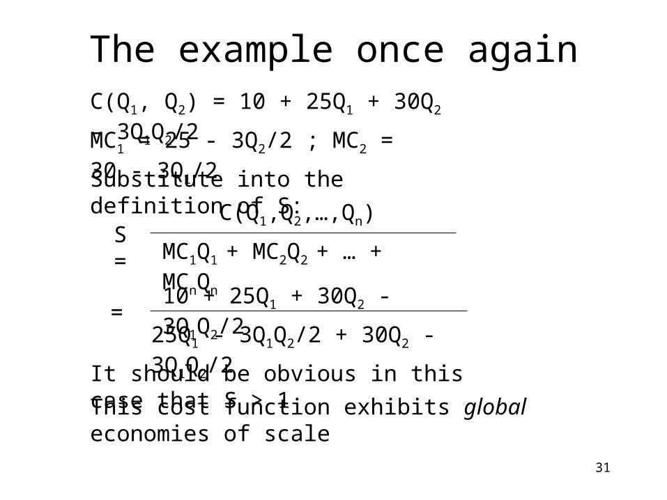
The example once againC(Q1, Q2) = 10 + 25Q1 + 30Q2 - 3Q1Q2/2

MC1 = 25 - 3Q2/2 ; MC2 = 30 - 3Q1/2

Substitute into the definition of S:

S =C(Q1,Q2,…,Qn)

MC1Q1 + MC2Q2 + … + MCnQn

=10 + 25Q1 + 30Q2 - 3Q1Q2/2

25Q1 - 3Q1Q2/2 + 30Q2 - 3Q1Q2/2

It should be obvious in this case that S > 1

This cost function exhibits global economies of scale

32

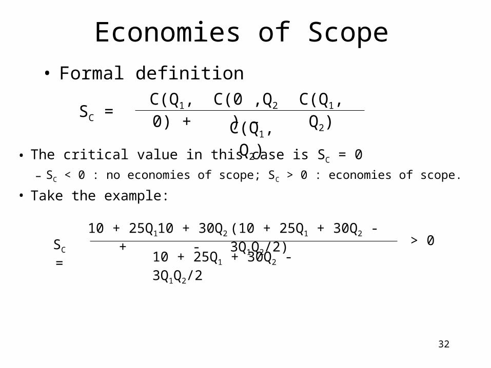
Economies of Scope• Formal definition

SC =C(Q1, 0) + C(0 ,Q2) - C(Q1, Q2)

C(Q1, Q2)

• The critical value in this case is SC = 0

– SC < 0 : no economies of scope; SC > 0 : economies of scope.

• Take the example:

SC =10 + 25Q1 + 10 + 30Q2 - (10 + 25Q1 + 30Q2 - 3Q1Q2/2)

10 + 25Q1 + 30Q2 - 3Q1Q2/2 > 0

33

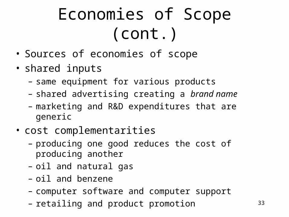
• Sources of economies of scope• shared inputs

– same equipment for various products

– shared advertising creating a brand name

– marketing and R&D expenditures that are generic

• cost complementarities– producing one good reduces the cost of producing another

– oil and natural gas

– oil and benzene

– computer software and computer support

– retailing and product promotion

Economies of Scope (cont.)

34

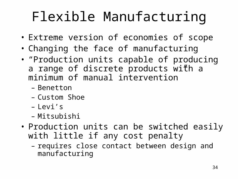
Flexible Manufacturing

• Extreme version of economies of scope• Changing the face of manufacturing• “Production units capable of producing a range of

discrete products with a minimum of manual intervention”– Benetton– Custom Shoe– Levi’s– Mitsubishi

• Production units can be switched easily with little if any cost penalty– requires close contact between design and manufacturing

35

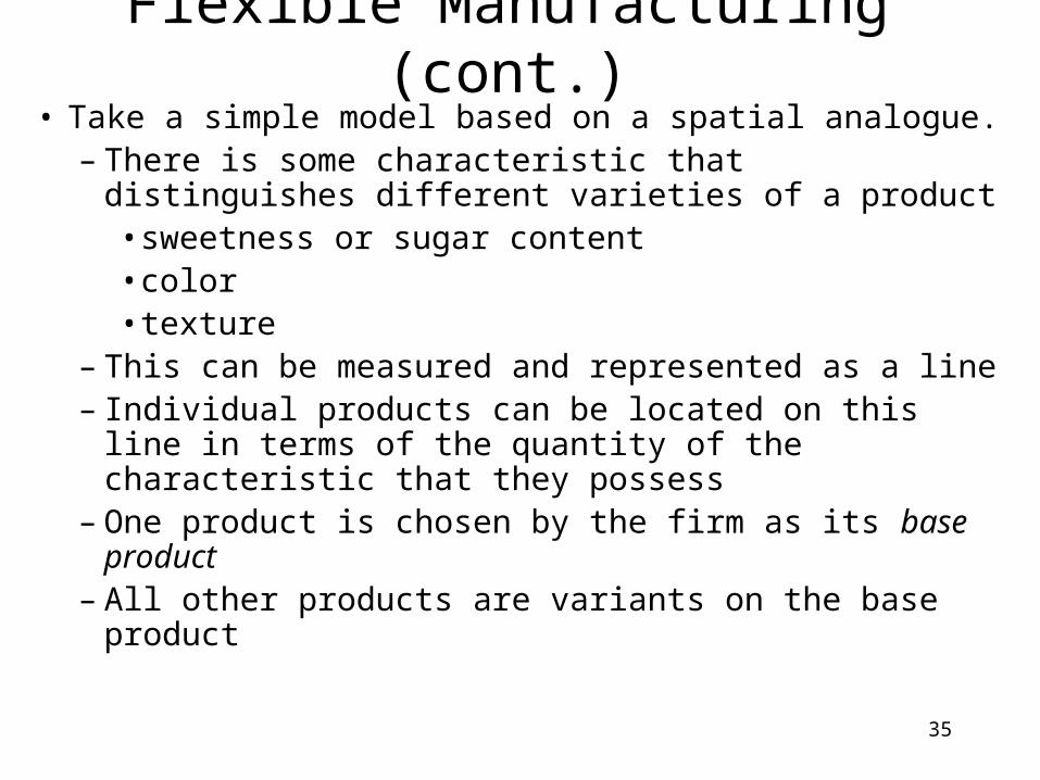
Flexible Manufacturing (cont.)• Take a simple model based on a spatial analogue.

– There is some characteristic that distinguishes different varieties of a product• sweetness or sugar content• color• texture

– This can be measured and represented as a line– Individual products can be located on this line in

terms of the quantity of the characteristic that they possess

– One product is chosen by the firm as its base product– All other products are variants on the base product

36

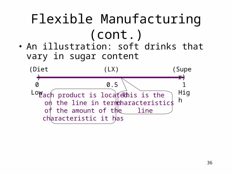
Flexible Manufacturing (cont.)

• An illustration: soft drinks that vary in sugar content

0 10.5

This is the characteristics

line

Each product is locatedon the line in termsof the amount of thecharacteristic it has

Low High

(Diet) (LX) (Super)

37

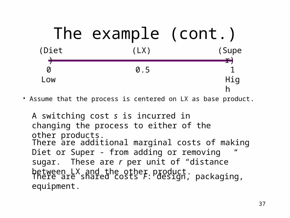
The example (cont.)

• Assume that the process is centered on LX as base product.

0 10.5Low High

(Diet) (LX) (Super)

A switching cost s is incurred in changing the process to either of the other products.

There are additional marginal costs of making Diet or Super - from adding or removing sugar. These are r per unit of “distance” between LX and the other product.

There are shared costs F: design, packaging, equipment.

38

The example (cont.)

• In the absence of shared costs there would be specialized firms.

• Shared costs introduce economies of scope.

Total costs are: C(zj, qj) = F + (m - 1)s + j=1

m[(c + rzj - z1)qj]

If production is 100 units of each product:

C3 = 3F + 300cone product per firm with three firms

one firm with all three products C1 = F + 2s + 300c + 100r

C1 < C3 if 2s + 100r < 2F F > 50r + s

This implies a constraint on set-up costs, switching costs and marginal costs for multi-product production to be preferred.

39

Economies of scale and scope

• Economies of scale and scope affect market structure but cannot be looked at in isolation.

• They must be considered relative to market size.

• Should see concentration decline as market size increases

• For example, entry to the medical profession is going to be more extensive in Chicago than in Oxford, Miss

40

Network Externalities

• Market structure is also affected by the presence of network externalities– willingness to pay by a consumer increases as the

number of current consumers increase• telephones, fax, Internet, Windows software• utility from consumption increases when there are more

current consumers

• These markets are likely to contain a small number of firms– even if there are limited economies of scale and scope

41

The Role of Policy

• Government can directly affect market structure– by limiting entry

• taxi medallions in Boston and New York

• airline regulation

– through the patent system– by protecting competition e.g. through the

Robinson-Patman Act