1 CFA Society Phoenix Wendell Licon, CFA CFA Level I Exam Tutorial 2014 Corporate Finance Power Point Slides

1

CFA Society PhoenixWendell Licon, CFA

CFA Level I Exam Tutorial 2014

Corporate Finance

Power Point Slides

2

Financial Management

Agency Problems• Bondholders vs. stockholders (managers)

– Occur when debt is risky– Managerial incentives to transfer wealth

• Management vs. stockholders– Occur when corporate governance system

does not work perfectly– Managerial incentives to extract private

benefits

3

Financial Management

Agency Problems

• Mechanisms to align management with shareholders– Compensation– Threat of firing– Direct intervention by shareholders

(CalPERS) – Takeovers

4

Cost of Capital

WACC = )1( cddpspscscs Tkwkwkw

)1( cdpscs Tkdpscs

dk

dpscs

psk

dpscs

cs

5

Cost of Capital

kd(1-Tc)

– Where do we get kd from?

6

Cost of Capital (debt)

Example: First find the market determined cost of issued debt:10-yr, 8% coupon bond, trades at $1,050, TC = .4

1,050 =

kd/2 = 3.644%, so kd = 7.288%

kd/2(1-Tc)= 3.644%(1-.4) = 2.1864% (semi-annual rate)

kd(1-Tc)=2.1864% * 2 = 4.3728% (annualized)

))1(

1(000,1)

)1(

111(40

202/

202/2/2/ dddd kkkk

7

Cost of Capital (debt with flotation costs)

Flotation Costs

Example: 2% of issue amount, coupon = 7.288% if issued at par (which is usually safe to assume), then

coupon rate = investor’s YTM

980 =

kd/2= 3.7885%

kd/2(1-Tc)= 3.7885%(1-.4) = 2.2731% (semi-annual rate)

kd(1-Tc)=2.2731% * 2 = 4.5462% (annualized)

))1(

1(000,1)

)1(

111(44.36

202/

202/2/2/ dddd kkkk

8

Cost of Capital (Preferred Shares)

Already in after-tax form

• Flotation Costs (F): kps= Divps/{P(1-F)}

• Example: P= 100, Divps= 10, F= 5%

• kps= 10/{100(1-.05)}= 10.526%

9

Cost of Capital (Common)

Discounted Cash Flow (DCF)

• Simple g assumption?• Cost of CS = Dividend Yield + Growth• Example: D1= 3/yr, P0 = 100, g= 12%

kcs = 15% • What about flotation costs? Multiply P0 by (1 –

F)

gP

Dk

gk

DP cs

cs

0

110

10


What about g?

g = ROE x (plowback ratio) or

g = ROE x (1 – payout rate)

11


Capital Asset Pricing Model (CAPM)

• kcs = krf + cs(km – krf)

12

WACC

• The market is impounding the current risks of the firm’s projects into the components of WACC

• Say Coca Cola’s WACC is 15%, which would be the rate associated with non-alcoholic beverages

• Can Coke use 15% to discount the cash flows for an alcoholic beverage project?

13

WACC

Coke Example cont’d– Say alcoholic beverage projects require 22%

returns– Security market line

14

WACC

15

WACC

Can be used for new projects if:– New project is a carbon copy of the firm’s

average project– Capital structure doesn’t materially change –

look at the WACC formula

16

WACC

• Don’t think of WACC as a static hurdle rate of return which, if cleared, then the project decision is a “go”

• If the firm changes its project mix, the WACC will change but the risk level of the projects already in progress will not & neither do the required rates of return for those projects

17

Cost of Capital- MCC

Step 1: Calculate how far the firms retained earnings will go before having to issue new common stock (layer 1)

• Example: Simple capital structure• LT Debt = 60% (yielding 8%)• CS = 40% (Kcs = 15%)• New Retained earnings (RE) = 1,000,000 (over

and above the 40%)• Marginal Tax Rate = 40%• Debt Flotation Costs = 1% per year• CS Flotation Costs = 1% per year

18


Concept: Keep our capital structure of 60%/40% in balance while utilizing our retained earnings slack matched with new debt, which is not in a slack condition

• Current WACC:

.6*(.08)*(1-.4) + .4*(.15) = 8.8%

19


How far can we go with Layer 2?1,000,000/.4 = 2,500,000 of new projects costs of

which2,500,000 * .6 = 1,500,000 in new issue debt

and 1,000,000 = use of retained earnings

• Layer 2 WACC:.6*(.09)*(1-.4) + .4(.15) = 9.24%

• Layer 3 would include new projects over 2,500,000 with flotation costs for equity and flotation costs for debt

20


Layer 3 WACC:

.6*(.09)*(1-.4) + .4(.16) = 9.64%

21

Cost of Capital Factors

Not in the firm’s control– Interest rates– Tax rates

Within the firm’s control– Capital structure policy– Dividend policy– Investment policy

22

Capital Budgeting

Payback Period– The amount of time it takes for us to recover

our initial outlay without taking into account the time value of money.

– The decision rule is to accept any project that has a payback period <= critical payback period (maximum allowable payback period), set by firm policy.

23

Capital Budgeting

Payback Period– Assume our maximum allowable payback

period is 4 years (nothing magical about 4 years as it is set by management):

Year Accum. Cash Flows1 5MM < 20MM2 5MM + 7 MM = 12MM <20MM3 12MM + 7MM = 19 MM <20MM4 19MM + 10MM = 29 MM >20MM

24

Capital Budgeting

Payback Period• Get paid back during the 4th year. We need

$1MM entering yr 4, and get $10MM for the whole year. If we assume $10MM comes evenly throughout the year, then we reach $20MM in {1MM/10MM} or .1 yrs.

• So, payback = 3.1 years.

• Do we accept or reject the project? Accept, since 3.1 < 4.

25

Capital Budgeting

Discounted Payback Period

• Discount each year’s cash flow to a present day valuation and then proceed as with Payback Period.

26

Capital Budgeting – Net Present Value

NPV = PV (inflows) - PV(outflows)

NPV = ACFt / (1 + k)t - IO ,

where, • IO = initial outlay

• ACFt = after-tax CF at t

• k = cost of capital (cost of capital for the firm)• n = project’s life

Decision rule: Accept all projects with NPV >= 0

27

Capital Budgeting - NPV

Accepting + NPV projects increases the value of the firm (higher stock value/equity), kind of like you are outrunning the cost of capital

28


Invest $100 in your 1-yr business. My required rate of return is 10%. What would be the CF be at the end of year 1 such that the NPV = 0?

• ACF1 = 100(1.1) = 110 (just the FV!)

• If NPV > 0, it is the same as ACFt > 110.

29


Ex: 120. Now, what’s the investment worth?

• Just PV of $120 = 120/1.1 = 109.09.

• My stock is now worth 109.09, a capital gain of 9.09 due to you accepting the project. (the 9.09 is the NPV = 120/1.1 - 100 = 9.09)

30

Capital Budgeting - IRR

IRR is our estimate of the return on the project. The definition of IRR is the discount rate that equates the present value of the project’s after-tax cash flows with the initial cash outlay.

• In other words, it’s the discount rate that sets the NPV equal to zero.

NPV = ACFt / (1 + IRR)t - IO = 0, or

ACFt / (1 + IRR)t = IO

• The decision criterion is to accept if IRR >= discount rate on the project.

31


Are the decision rules the same for IRR & NPV? Think about a project that has an IRR of 15% and a required rate of return (cost of capital) of 10%. So, we should accept the project.

32


What is the NPV of the project if we discount the CF at 15%? – Zero - by definition of IRR. Is the PV of the

CF’s going to be higher or lower if the rate is 10%? Higher - lower rate means higher PV. So, the sum term is bigger at 10%, so the NPV is positive ===> accept.

NPV and IRR will accept and reject the same projects – the only difference is when ranking projects.

33


Computing IRR: Case 1 - even cash flows

• Ex. IO = 5,000, Cft = 2,000/yr for 3 years

IO = CF(PVIFA IRR,3) ===> 5,000 = 2,000(PVIFA IRR,3)

Just find the factor for n=3 that = 5,000/2,000 = 2.5• For i=9, PVIFA = 2.5313• For i=10, PVIFA = 2.4869• It’s between 9 & 10: additional work gives 9.7%

34


Case 2 Uneven CF’s - even worse• Trial and Error!

• Ex: IO = 20,000, CF1 = 5,000, CF2 = 7,000, CF3 = 7,000, CF4 = 10,000, CF5 = 10,000

• We have to find IRR such that

• 0 = 5,000 (PVIF IRR,1) + 7,000 (PVIF IRR,2) + 7,000 (PVIF IRR,3) + 10,000 (PVIF IRR,4) + 10,000 (PVIF

IRR,5) – 20,000

35


• NPV at 25% is -563. So, should we try a higher or lower rate?

Lower (==> higher NPV) If we try 24%, we get NPV = -102.97, at 23%,

we get NPV = 375

==> it’s between 23 & 24%. A final answer gives 23.8%.

36


IRR has same advantages as NPV and the same disadvantages, plus

1. Multiple IRRs: IRR involves solving a polynomial. There are as many solutions as there are sign changes in the cash flows. In our previous example, one sign change. If you had a negative flow at t6 ==> 2 changes ==> 2 IRRs. Neither one is necessarily any good.

2. Reinvestment assumption: IRR assumes that intermediate cash flows are reinvested at the IRR. NPV assumes that they are reinvested at k (Required Rate of Return). Which is better? Generally k. Can get around the IRR problem by using the Modified IRR, MIRR.

37


1. Multiple IRRs:

2. Reinvestment assumption:

38

Capital Budgeting - MIRR

• Used when reinvestment rate especially critical • Idea: instead of assuming a reinvestment rate =

IRR, use reinvestment rate = k (kind of do this manually), then solve for rate of return.

• 1st: separate outflows and inflows– Take outflows back to present at a k discount rate– Roll inflows forward - “reinvest” them - at the cost of

capital, until the end of the project (n) - now just have one big terminal payoff at n.

• The MIRR is the rate that equates the PV of the outflows with the PV of these terminal payoffs.

39


40


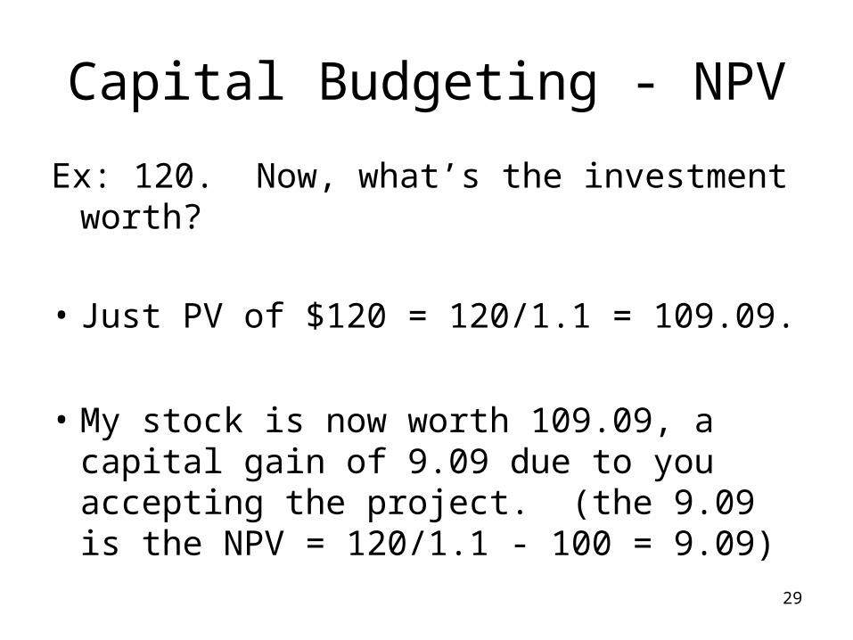
ACOFt/(1 + k)t = ( ACIFt* (1 + k) n-t) / (1 + MIRR) n

where ACOF = after-tax cash outflows,

ACIF = after-tax cash inflows.

Solve for MIRR.

MIRR >= k (cost of capital) ==> accept

41


• Notice, now just one sign change with no multiple rate problems –

one positive MIRR

• Plus, no reinvestment problem

• Still expressed as a % which people like

• Also, much easier to solve

42

Capital Budgeting - MIRR Ex: Initial outlay = 20,000, plus yr. 5 CF = -10,000. We’ll use k=12%Draw timeline1. PV of outflows = 20,000 + 10,000(1/1.12)5 = 25,6742. FV of inflows: yr. 1 CF = 5,000; yr. 2 and 3 CF = 7,000; yr. 4 CF =

10,000;YR FV1 5,000(1.12 ) 5-1 = 5,000(1.12 )4 = 7,8682 7,000 (1.12 ) 5-2 = 7,000(1.12 )3 = 9,8343 7,000 (1.12 ) 5-3 = 7,000(1.12 )2 = 8,7814 10,000(1.12 ) 5-4 = 10,000(1.12 )1 = 11,200

-------------Sum 37,683

43

Capital Budgeting Decision Criteria

• So, NPV and IRR all give same accept/reject decisions. But, they will rank projects differently

• When is ranking important?

• Capital rationing - firm has fixed investment budget, no matter how many + NPV projects there are out there.

44


Ex. firm has $5MM – If firm used IRR to rank, would pick highest

IRR projects, next highest, etc., until spent $5MM. With NPV, pick projects to maximize total NPV subject to not spending more than $5MM.

Mutually exclusive projects - just means can’t do both. Which do we pick - highest NPV or IRR?

45


• It’s easiest to see ranking problems through NPV profile - just a graph of NPV vs. discount rates:

• By NPV: for k < 10%, pick A. For k > 10% pick B

46


• IRR: always pick B

• NPV better: it incorporates our k, it’s how much we’re adding to shareholder value. If k < 10%, IRR gives wrong decision.

47

Capital Budgeting Post-Audit

• Compare actual results to forecast

• Explain variances

48

Cash Flows in Capital Budgeting

Cash flow is important, not Accounting Profits

• Net Cash Flow = NI + Depreciation

49


• Incremental Cash Flows are what is important– Ignore sunk costs– Don’t ignore opportunity costs (think of next

best alternative)– What about externalities (the effect of this

project on other parts of the firm), and cannibalization

– Don’t forget shipping and installation (capitalized for depreciation)

50


Changes in Net Working Capital– Remember to reverse this out at the end of

the project– Example: think of petty cash

51


Projects with Unequal lives – 2 solutions

• Replacement Chain – like finding lowest common denominator

• Equivalent annual annuity – like finding how fast the cash is flowing in to the firm

52


What if projects have different lives?Machine #1: cost = 24,000, life 4 yrs, net benefits =

$8,000/yearMachine #2: cost = 12,000, life 2 yrs, net benefits =

$7,400/yeark = 10%

NPV1 = -24,000 + 8,000 PVIFA( 10%,4)= 1,359NPV2 = -12,000 + 7,400 PVIFA(10%,2)= 843

We cannot compare these like this, since have unequal lives.

53


1. Replacement chain approach. Construct a chain of #2’s to get the same number of years of benefits (like finding least common denominator):

Year 0 1 2 3 4Inflows 7400 7400 7400 7400Outflows -12000 -12000

Net CF -12000 7400 -4600 7400 7400NPV2 = 1,540- so we choose machine #2, not #1

54


2. Equivalent annual annuity. Find the annual payment of an annuity that lasts as long as the project & whose PV equals the NPV of the project

Project 1: NPV = EAA (PVIFA 10%,4) ==> EAA = 1,359/(PVIFA 10%,4) =1359/3.1699 = 428.72

Project 2: NPV = EAA (PVIFA 10%,2) ==> EAA = 843/1.7355 =485.74

55


Dealing with Inflation

• As long as inflation is built into your cash flow forecast, you are OK because your discount rates should already take expected inflation into account

56

Risk Analysis

Types of Risk

• Stand-alone risk – think total risk or variance (or standard deviation)

• Corporate (within firm) risk – think of the firm as a portfolio of projects but not a completely diversified portfolio

• Market risk – think systematic or beta

57

Risk Analysis

Modeling Methods• Sensitivity Analysis

– Find the effect of a change due to a single variable change at a time

• Scenario Analysis– Find the effect of many simultaneous changes

(brought on by different scenarios)

• Monte Carlo Simulation– Find the distributional effect of a number of random

changes on repeated attempts

58

Risk Analysis

Market Risk• Security Market Line

– kcs = krf + cs(km – krf)

• Measuring Beta– The pure play method

• Find a market traded firm whose only business is what you are interested in

– Accounting beta method• Accounting ROA of firm versus Average Accounting ROA for

market construct (Text says S&P 400)

59

Risk Analysis

Investment Opportunity Schedule vs Marginal Cost of Capital

60

Capital Structure and Leverage

Factors influencing a firm’s decision:

• Business risk - DOL

• Taxes

• Financial flexibility - DFL

• Managerial conservatism – risk aversion

61


Business Risk

• Break-even Operating Quantity

• Degree of Operating Leverage (DOLS)– A measure of the degree to which fixed costs

are used

• High Fixed Costs ===> High Operating Leverage

FVPQ

VPQ

FVCS

VCSor

Sales

EBITDOLs

)(

)(

%

%

VP

FQBE

62


Financial Risk

• Degree of Financial Leverage (DFLEBIT)

• A measure of the degree to which debt is used

• The higher the firm relies on debt, the greater the DFL will be

IEBIT

EBIT

IFVPQ

FVPQor

EBIT

EPSDFLEBIT

)(

)(

%

%

63


Combined Risk

• Degree of Total Leverage (DTLS)

– Measure of the combined leverage utilized by a firm

• DCLS = [DOLS] X [DFLEBIT]

IFVPQ

VPQor

Sales

EPSDCLS

)(

)(

%

%

64


• Miller and Modigliani 1958

• The value of the firm is independent of its capital structure, i.e., the financing mix is irrelevant (Miller and Modigliani 1958)

• Proposition: VU = VL

65


Assumptions• Perfect capital markets

– No taxes– No transaction costs– Borrow and lend at the same rate

• No bankruptcy costs• Homogenous preferences and beliefs• Firm issued debt is risk-free (no chance of

bankruptcy)

66


Relax the Assumptions

• Introduce Taxes – more debt is better

• Relax no bankruptcy assumption – at some point, more debt reduces the value of the firm

• The above is really trade-off theory

67


Effect of WACC

)1( cddpspscscs Tkwkwkw

68


Signaling Theory• Signals must be costly

– New equity issue signal– New debt issue signal

69

Dividend Policy

• Dividend policy must strike a balance between future growth and the need to pay investors cash

• M&M irrelevance (homemade dividends)• g = ROE x (1 – payout ratio)• Signaling through dividends

70

Dividend Policy

• Residual Dividend Model– Dividend policy set to pay out cash that is not need

for investment or for reserve cash reasons

71

Dividend Policy

Timing• Declaration date – declared by the board• Holder-of-record-date – the last date that a

person can hold the stock and still receive the dividend

• Ex-dividend date – the first date that a stock trades without rights to the dividend

• Payment date

72

Dividend Policy

Stock Dividends and Splits• Splits: increasing the number of shares by a

multiple• Dividends: the dividend is paid in stock

instead of cash• Price effects of stock dividends and splits

– Prices generally rise after the announcement– Signal? Higher cash dividends in the future?

73

Dividend Policy

Repurchases• Advantages:

– Positive signal to repurchases shares– Targeted dividends– Remove a large block– Get cash in investors hands without future

expectations– Capital structure changes

• Disadvantages– Investor indifference, informational asymmetry

among investors, paying to high a price for shares

Documents

1 CFA Society Phoenix Wendell Licon, CFA CFA Level I Exam Tutorial 2014 Corporate Finance Power Point Slides