Embed Size (px)
Citation preview
1
Capacity of the Trapdoor Channel withFeedback
Haim Permuter, Paul Cuff, Benjamin Van Roy and Tsachy Weissman
Abstract
We establish that the feedback capacity of the trapdoor channel is the logarithm of the golden ratio and providea simple communication scheme that achieves capacity. As part of the analysis, we formulate a class of dynamicprograms that characterize capacities of unifilar finite-state channels. The trapdoor channel is an instance that admitsa simple analytic solution.
Index Terms
Bellman equation, chemical channel, constrained coding, directed information, feedback capacity, golden-ratio,infinite-horizon dynamic program, trapdoor channel, value iteration.
I. INTRODUCTION
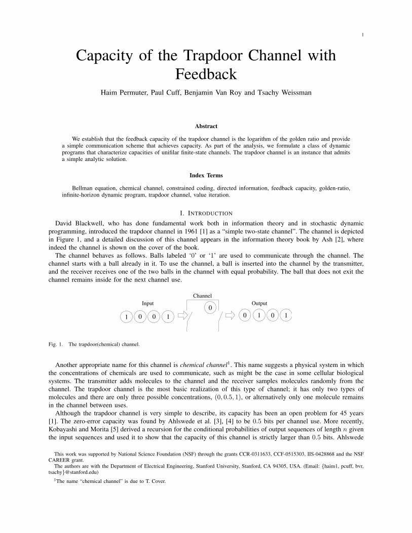
David Blackwell, who has done fundamental work both in information theory and in stochastic dynamicprogramming, introduced the trapdoor channel in 1961 [1] as a “simple two-state channel”. The channel is depictedin Figure 1, and a detailed discussion of this channel appears in the information theory book by Ash [2], whereindeed the channel is shown on the cover of the book.
The channel behaves as follows. Balls labeled ‘0’ or ‘1’ are used to communicate through the channel. Thechannel starts with a ball already in it. To use the channel, a ball is inserted into the channel by the transmitter,and the receiver receives one of the two balls in the channel with equal probability. The ball that does not exit thechannel remains inside for the next channel use.
00
1 1 00 1 1
OutputInputChannel
0
Fig. 1. The trapdoor(chemical) channel.
Another appropriate name for this channel is chemical channel1. This name suggests a physical system in whichthe concentrations of chemicals are used to communicate, such as might be the case in some cellular biologicalsystems. The transmitter adds molecules to the channel and the receiver samples molecules randomly from thechannel. The trapdoor channel is the most basic realization of this type of channel; it has only two types ofmolecules and there are only three possible concentrations, (0, 0.5, 1), or alternatively only one molecule remainsin the channel between uses.
Although the trapdoor channel is very simple to describe, its capacity has been an open problem for 45 years[1]. The zero-error capacity was found by Ahlswede et al. [3], [4] to be 0.5 bits per channel use. More recently,Kobayashi and Morita [5] derived a recursion for the conditional probabilities of output sequences of length n giventhe input sequences and used it to show that the capacity of this channel is strictly larger than 0.5 bits. Ahlswede
This work was supported by National Science Foundation (NSF) through the grants CCR-0311633, CCF-0515303, IIS-0428868 and the NSFCAREER grant.
The authors are with the Department of Electrical Engineering, Stanford University, Stanford, CA 94305, USA. (Email: {haim1, pcuff, bvr,tsachy}@stanford.edu)
1The name “chemical channel” is due to T. Cover.
2
and Kaspi [3] considered two modes of the channel called the permuting jammer channel and the permuting relaychannel. In the first mode there is a jammer in the channel who attempts to frustrate the message sender by selectiverelease of balls in the channel. In the second mode, where the sender is in the channel, there is a helper supplyingballs of a fixed sequence at the input, and the sender is restricted to permuting this sequence. The helper collaborateswith the message sender in the channel to increase his ability to transmit distinct messages to the receiver. Ahlswedeand Kaspi [3] gave answers for specific cases of both situations and Kobayashi [6] established the answer to thegeneral permuting relay channel. More results for specific cases of the permuting jammer channel can be found in[7], [8].
In this paper we consider the trapdoor channel with feedback. We derive the feedback capacity of the trapdoorchannel by solving an equivalent dynamic programming problem. Our work consists of two main steps. The firststep is formulating the feedback capacity of the trapdoor channel as an infinite-horizon dynamic program, and thesecond step is finding explicitly the exact solution of that program.
Formulating the feedback capacity problem as a dynamic program appeared in Tatikonda’s thesis [9] and in workby Yang, Kavcic and Tatikonda [10], Chen and Berger [11], and recently in a work by Tatikonda and Mitter [12].Yang et. al. [10] have shown that if a channel has a one-to-one mapping between the input and the state, it ispossible to formulate feedback capacity as a dynamic programming problem and to find an approximate solution byusing the value iteration algorithm [13]. Chen and Berger [11] showed that if the state of the channel is a functionof the output then it is possible to formulate the feedback capacity as a dynamic program with a finite number ofstates.
Our work provides the dynamic programming formulation and a computational algorithm for finding the feedbackcapacity of a family of channels called unifilar Finite State Channels (FSC’s), which include the channels consideredin [10], [11]. We use value iteration [13] to find an approximate solution and to generate a conjecture for the exactsolution, and the Bellman equation [14] to verify the optimality of the conjectured solution. As a result, we are ableto show that the feedback capacity of the trapdoor channel is log φ, where φ is the golden ratio, 1+
√5
2 . In addition,we present a simple encoding/decoding scheme that achieves this capacity. The remainder of the paper is organizedas follows. Section II defines the channel setting and the notation throughout the paper. Section III states the mainresults of the paper. Section IV presents the capacity of a unifilar FSC in terms of directed information. SectionV introduces the dynamic programming framework and shows that the feedback capacity of the unifilar FSC canbe characterized as the optimal average reward of a dynamic program. Section VI shows an explicit solution forthe capacity of the trapdoor channel by using the dynamic programming formulation. Section VII gives a simplecommunication scheme that achieves the capacity of the trapdoor channel with feedback and finally Section VIIIconcludes this work.
II. CHANNEL MODELS AND PRELIMINARIES
We use subscripts and superscripts to denote vectors in the following ways: xj = (x1 . . . xj) and xji = (xi . . . xj)for i ≤ j. Moreover, we use lower case x to denote sample values, upper case X to denote random variables,calligraphic letter X to denote the alphabet and |X | to denote the cardinality of the alphabet. The probabilitydistributions are denoted by p when the arguments specify the distribution, e.g. p(x|y) = p(X = x|Y = y). Inthis paper we consider only channels for which the input, denoted by {X1, X2, ...}, and the output, denoted by{Y1, Y2, ...}, are from finite alphabets, X and Y , respectively. In addition, we consider only the family of FSCknown as unifilar channels as considered by Ziv [15]. An FSC is a channel that, for each time index, has one ofa finite number of possible states, st−1, and has the property that p(yt, st|xt, st−1, yt−1) = p(yt, st|xt, st−1). Aunifilar FSC also has the property that the state st is deterministic given (st−1, xt, yt):
Definition 1: An FSC is called a unifilar FSC if there exists a time-invariant function f(·) such that the stateevolves according to the equation
st = f(st−1, xt, yt). (1)We also define a strongly connected FSC, as follows.
Definition 2: We say that a finite state channel is strongly connected if for any state s there exists an integerT and an input distribution of the form {p(xt|st−1)}Tt=1 such that the probability that the channel reaches state sfrom any starting state s′, in less than T time-steps, is positive. I.e.
T∑
t=1
Pr(St = s|S0 = s′) > 0, ∀s ∈ S,∀s′ ∈ S. (2)

3
PSfrag replacements
m
Message
Encoder
xt(m, yt−1)
xt
Unifilar Finite State Channel
p(yt|xt, st−1)
st = f(st−1, xt, yt) ytm
Decoder
m(yN )
yt
ytUnit Delay
yt−1
Feedback
message
m
Estimated
Fig. 2. Unifilar FSC with feedback
We assume a communication setting that includes feedback as shown in Fig. 2. The transmitter (encoder) knowsat time t the message m and the feedback samples yt−1. The output of the encoder at time t is denoted by xtand is a function of the message and the feedback. The channel is a unifilar FSC and the output of the channel ytenters the decoder (receiver). The encoder receives the feedback sample with one unit delay.
A. Trapdoor Channel is a Unifilar FSC
The state of the trapdoor channel, which is described in the introduction and shown in figure 1, is the ball, 0 or1, that is in the channel before the transmitter transmits a new ball. Let xt ∈ {0, 1} be the ball that is transmittedat time t and st−1 ∈ {0, 1} be the state of the channel when ball xt is transmitted. The probability of the outputyt given the input xt and the state of the channel st−1 is shown in table I.
TABLE ITHE PROBABILITY OF THE OUTPUT yt GIVEN THE INPUT xt AND THE STATE st−1 .
xt st−1 p(yt = 0|xt, st−1) p(yt = 1|xt, st−1)
0 0 1 00 1 0.5 0.51 0 0.5 0.51 1 0 1
The trapdoor channel is a unifilar FSC. It has the property that the next state st is a deterministic function of thestate st−1, the input xt, and the output yt. For a feasible tuple, (xt, yt, st−1), the next state is given by the equation
st = st−1 ⊕ xt ⊕ yt, (3)
where ⊕ denotes the binary XOR operation.
B. Trapdoor Channel is a Permuting Channel
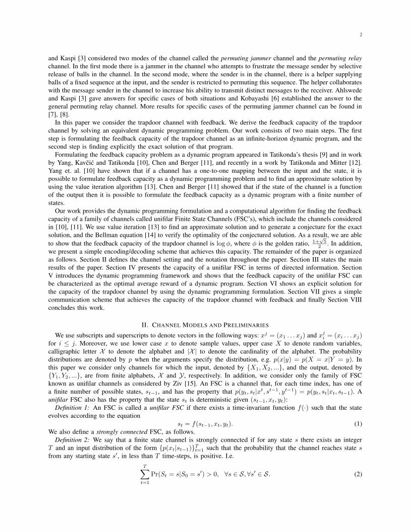
It is interesting to note, although not consequential in this paper, that the trapdoor channel is a permuting channel[16], where the output is a permutation of the input (Fig. 3). At each time t, a new bit is added to the sequenceand the channel switches the new bit with the previous one in the sequence with probability 0.5.
III. MAIN RESULTS
• The capacity of the trapdoor channel with feedback is
C = log
√5 + 1
2. (4)
4
0.5
0 1 001 0
0.5 0.5 0.5 0.5 0.5
1
Fig. 3. The trapdoor channel as a permuting channel. Going from left to right, there is a probability of one half that two adjacent bits switchplaces.
Furthermore, there exists a simple capacity achieving scheme which will be presented in Section VII.• The problem of finding the capacity of a strongly connected unifilar channel (Fig. 2) can be formulated as an
average-reward dynamic program, where the state of the dynamic program is the probability mass functionover the states conditioned on prior outputs, and the action is the stochastic matrix p(x|s). By finding a solutionto the average-reward Bellman equation we find the exact capacity of the channel.
• As a byproduct of our analysis we also derive a closed form solution to an infinite horizon average-rewarddynamic program with a continuous state-space.
IV. THE CAPACITY FORMULA FOR A UNIFILAR CHANNEL WITH FEEDBACK
The main goal of this section is to prove the following theorem which allows us to formulate the problem as adynamic program.
Theorem 1: The feedback capacity of a strongly connected unifilar FSC when initial state s0 is known at theencoder and decoder can be expressed as
CFB = sup{p(xt|st−1,yt−1)}t≥1
lim infN→∞
1
N
N∑
t=1
I(Xt, St−1;Yt|Y t−1) (5)
where {p(xt|st−1, yt−1)}t≥1 denotes the set of all distributions such that p(xt|yt−1, xt−1, st−1) = p(xt|st−1, y
t−1)for t = 1, 2, ... .
Theorem 1 is a direct consequence of Theorem 3 and eq. (26) in Lemma 4, which are proved in this section.For any finite state channel with perfect feedback, as shown in Figure 2, the capacity was shown in [17], [18]
to be bounded as
limN→∞
1
Nmax
p(xN ||yN−1)maxs0
I(XN → Y N |s0) ≥ CFB ≥ limN→∞
1
Nmax
p(xN ||yN−1)mins0
I(XN → Y N |s0). (6)
The term I(XN → Y N ) is the directed information2 defined originally by Massey in [25] as
I(XN → Y N ) ,N∑
t=1
I(Xt;Yt|Y t−1). (7)
The initial state is denoted as s0 and p(xN ||yN−1) is the causal conditioning distribution defined [17], [22] as
p(xN ||yN−1) ,N∏
t=1
p(xt|xt−1, yt−1). (8)
The directed information in eq. (6) is under the distribution of p(xn, yn) which is uniquely determined by the causalconditioning, p(xN ||yN−1), and by the channel.
In our communication setting we are assuming that the initial state is known both to the decoder and to theencoder. This assumption allows the encoder to know the state of the channel at any time t because st is adeterministic function of the previous state, input and output. In order to take into account this assumption, we usea trick of allowing a fictitious time epoch before the first actual use of the channel in which the input does notinfluence the output nor the state of channel and the only thing that happens is that the output equals s0 and is
2In addition to feedback capacity, directed information has recently been used in rate distortion [19], [20], [21], network capacity [22], [23]and computational biology [24].
5
fed back to the encoder such that at time t = 1 both the encoder and the decoder know the state s0. Let t = 0be the fictitious time before starting the use of the channel. According to the trick, Y0 = S0 and the input X0 canbe chosen arbitrarily because it does not have any influence whatsoever. For this scenario the directed informationterm in eq. (6) becomes
I(XN0 → Y N0 |s0) = I(XN → Y N |s0). (9)
The input distribution becomesp(xN0 ||{s0, y
N−1}) = p(xN ||yN−1, s0), (10)
where p(xN ||yN−1, s0) is defined as p(xN ||yN−1, s0) ,∏Nt=1 p(xt|xt−1, yt−1, s0). Therefore, the capacity of a
channel with feedback for which the initial state, s0, is known both at the encoder and the decoder is bounded as
limN→∞
1
Nmax
p(xN ||yN−1,s0)maxs0
I(XN → Y N |s0) ≥ CFB ≥ limN→∞
1
Nmax
p(xN ||yN−1,s0)mins0
I(XN → Y N |s0) (11)
Lemma 2: If the finite state channel is strongly connected, then for any input distribution p1(xN ||yN−1, s0) andany s′0 there exists an input distribution p2(xN ||yN−1, s′0) such that
1
N
∣∣Ip1(XN → Y N |s0)− Ip2
(XN → Y N |s′0)∣∣ ≤ c
N(12)
where c is a constant that does not depend on N , s0, s′0. The term Ip1(XN → Y N |s0) denotes the directed
information induced by the input distribution p1(xN ||yN−1, s0) where s0 is the initial state. Similarly, the termIp2
(XN → Y N |s′0) denotes the directed information induced by the input distribution p2(xN ||yN−1, s′0) where s′0is the initial state.
Proof: Construct p2(xN ||yN , s′0) as follows. Use an input distribution, which has a positive probability ofreaching s0 in T time epochs, until the time that the channel first reaches s0. Such an input distribution existsbecause the channel is strongly connected. Denote the first time that the state of the channel equals s0 by L.After time L, operate exactly as p1 would (had time started then). Namely, for t > L, p2(xt|xt−1, yt−1, s0) =p1(xt−L|xt−L−1, yt−L−1, s0). Then
1
N
∣∣Ip1(XN → Y N |s0)− Ip2
(XN → Y N |s′0)∣∣
(a)
≤ 1
N
∣∣Ip1(XN → Y N |s0)− Ip2
(XN → Y N |L, s′0)∣∣+
1
NH(L)
(b)=
1
N
∣∣∣∣∣∞∑
l=1
p(L = l)Ip1(XN → Y N |s0)−
∞∑
l=1
p(L = l)(Ip2
(XNl → Y Nl |sl) + Ip2
(X l → Y l|sl, s′0))∣∣∣∣∣+
1
NH(L)
(c)
≤ 1
N
∣∣∣∣∣∞∑
l=1
p(L = l)Ip1(XN → Y N |s0)−
∞∑
l=1
p(L = l)Ip2(XN
l → Y Nl |sl)∣∣∣∣∣
+1
N
∣∣∣∣∣∞∑
l=1
p(L = l)Ip2(X l → Y l|sl, s′0)
∣∣∣∣∣+1
NH(L)
(d)
≤ 2
N
∞∑
l=1
p(L = l)l log |Y|+ 1
NH(L)
=1
N(log |Y|E[L] +H(L)) (13)
(a) from the triangle inequality and Lemma 3 in [17] which claims that for an arbitrary random variables(XN , Y N , S), the inequality
∣∣I(XN → Y N )− I(XN → Y N |S)∣∣ ≤ H(S) always holds.
(b) follows from using the special structure of p2(xN ||yN , s′0).(c) follows from the triangle inequality.(d) follows from the fact that in the first absolute value N− l terms cancel and therefor only l terms remain where
each one of them is bounded by I(X t;Yt|Y t−1) ≤ |Y|. In the second absolute value there are l terms alsobounded by |Y|.
6
The proof is completed by noting that H(L) and E(L) are upper bounded respectively, by H(L) and E(L) wherebL/T c ∼ Geometric(p) and p is the minimum probability of reaching s0 in less than T steps from any state s ∈ S.Because the random variable bL/T c has a geometric distribution, H(L) and E[L] are finite and, consequently, soare H(L) and E(L).
Theorem 3: The feedback capacity of a strongly connected unifilar FSC when initial state is known at the encoderand decoder is given by
CFB = limN→∞
1
Nmax
{p(xt|st−1,yt−1)}Nt=1
N∑
t=1
I(Xt, St−1;Yt|Y t−1), (14)
Proof: The proof of the theorem contains four main equalities which are proven separately.
CFB = limN→∞
1
Nmax
p(xN ||yN−1,s0)mins0
I(XN → Y N |s0) (15)
= limN→∞
1
Nmax
p(xN ||yN−1,s0)I(XN → Y N |S0) (16)
= limN→∞
1
Nmax
p(xN ||yN−1,s0)
N∑
t=1
I(Xt, St−1;Yt|Y t−1) (17)
= limN→∞
1
Nmax
{p(xt|st−1,yt−1)}Nt=1
N∑
t=1
I(Xt, St−1;Yt|Y t−1). (18)
Proof of equality (15) and (16): As a result of Lemma 2,
limN→∞
1
Nmax
p(xN ||yN−1,s0)I(XN → Y N |S0)
(a)= lim
N→∞1
Nmax
p(xN ||yN−1,s0)
∑
s0
p(s0)I(XN → Y N |s0)
(b)= lim
N→∞1
N
∑
s0
p(s0) maxp(xN ||yN−1,s0)
I(XN → Y N |s0)
(c)= lim
N→∞1
Nmins0
maxp(xN ||yN−1,s0)
I(XN → Y N |s0) (19)
(d)= lim
N→∞1
Nmax
p(xN ||yN−1,s0)mins0
I(XN → Y N |s0). (20)
where,
(a) follows from the definition of conditional entropy.(b) follows from exchanging between the summation and the maximization. The exchange is possible because
maximization is over causal conditioning distributions that depend on s0 .(c) follows from Lemma 2.(d) follows from the observation that the distribution p∗(xN ||yN−1, s0) that achieves the maximum in (19) and in
(20) is the same: p∗(xN ||yN−1, s0) = arg maxp(xN ||yN−1,s0) I(XN → Y N |s0). This observation allows us toexchange the order of the minimum and the maximum.
Equations (19) and (20) can be repeated also with maxs0 instead of mins0 and hence we get
limN→∞
1
Nmax
p(xN ||yN−1,s0)I(XN → Y N |S0) = lim
N→∞1
Nmax
p(xN ||yN−1,s0)maxs0
I(XN → Y N |s0). (21)
By using eq. (20) and (21), we get that the upper bound and lower bound in (11) are equal and therefore eq.(15) and (16) hold.
7
Proof of equality (17): Using the property that the next state of the channel is a deterministic function of theinput, output and current state we get,
I(XN → Y N |S0) =
N∑
t=1
I(Xt;Yt|Y t−1, S0)
=
N∑
t=1
H(Yt|Y t−1, S0)−H(Yt|Xt, Y t−1, S0)
(a)=
N∑
t=1
H(Yt|Y t−1, S0)−H(Yt|Xt, Y t−1, S0, St−1(Xt, Y t−1, S0))
(b)=
N∑
t=1
H(Yt|Y t−1, S0)−H(Yt|Xt, St−1, Yt−1, S0)
=N∑
t=1
I(St−1, Xt;Yt|Y t−1, S0). (22)
Equality (a) is due to the fact that st−1 is a deterministic function of the tuple (xt, yt−1, s0). Equality (b) is due tothe fact that p(yt|xt, yt−1, st−1, s0) = p(yt|xt, yt−1, st−1, s0). By combining eq. (16) and eq. (22) we get eq. (17).
Proof of equality (18): It will suffice to prove by induction that if we have two input distributions{p1(xt|xt−1, yt−1, s0)}t≥1 and {p2(xt|xt−1, yt−1, s0)}t≥1 that induce the same distributions {p(xt|st−1, y
t−1)}t≥1
then the distributions {p(st−1, xt, yt)}t≥1 are equal under both inputs. First let us verify the equality for t = 1:
p(s0, x1, y1) = p(s0)p(x1|s0)p(y1|s0, x1). (23)
Since p(s0) and p(y1|s0, x1) are not influenced by the input distribution and since p(x1|s0) is equal for both inputdistributions then p(s0, x1, y1) is also for both input distributions. Now, we assume that p(st−1, xt, y
t) is equal underboth input distributions and we need to prove that p(st, xt+1, y
t+1) is also equal under both input distributions.The term p(st, xt+1, y
t+1) which can be written as,
p(st, xt+1, yt+1) = p(st, y
t)p(xt+1|st, yt)p(yt+1|xt+1, st). (24)
First we notice that if p(st−1, xt, yt) is equal for both cases then necessarily p(st−1, st, xt, y
t) is also equal forboth cases because st is a deterministic function of the tuple (st−1, xt, yt) and therefore both input distributionsinduce the same p(st, yt). The distribution, p(xt+1|st, yt), is the same under both input distributions by assumptionand p(yt+1|xt+1, st) does not depend on the input distribution.
The next lemma shows that it is possible to switch between the limit and the maximization in the capacityformula. This is necessary for formulating the problem, as we do in the next section, as an average-reward dynamicprogram.
Lemma 4: For any FSC the following equality holds:
limN→∞
1
Nmax
p(xN ||yN−1,s0)mins0
I(XN → Y N |s0) = sup{P (xt|yt−1,xt−1,s0)}t≥1
lim infN→∞
1
Nmins0
I(XN → Y N |s0). (25)
And, in particular, for a strongly connected unifilar FSC
limN→∞
1
Nmax
{p(xt|st−1,yt−1)}Nt=1
N∑
t=1
I(Xt, St−1;Yt|Y t−1) = sup{p(xt|st−1,yt−1)}t≥1
lim infN→∞
1
N
N∑
t=1
I(Xt, St−1;Yt|Y t−1)
(26)
On the left-hand side of the equations appears lim because, as shown in [18], the limit exists due to the super-additivity property of the sequence.
Proof: We are going to prove eq. (25) which hold for any FSC. For the case of unifilar channel, the left-handside of eq. (25) is proven to be equal to the left side of eq. (26) in eq. (15)-(18). By the same arguments as in(15)-(18) also the right-hand side of (25) and (26) are equal.
8
DefineCN ,
1
Nmax
p(xN ||yN−1,s0)mins0
I(XN → Y N |s0). (27)
In order to prove that the equality holds we will use two properties of CN that were proved in [18, Theorem13].
The first property, is that CN is a super additive sequence, namely,
N
[CN −
log |S|N
]≥ n
[Cn −
log |S|n
]+ l
[Cl −
log |S|l
]. (28)
The second property, which is a result of the first, is that
limN→∞
CN = supNCN (29)
Now, consider
limN→∞
1
Nmax
p(xN ||yN−1,s0)mins0
I(XN → Y N |s0) = supNCN
= supN
1
Nmax
p(xN ||yN−1,s0)mins0
I(XN → Y N |s0)
= supN
1
Nsup
{p(xt|yt−1,xt−1,s0)}t≥1
mins0
I(XN → Y N |s0)
= sup{p(xt|yt−1,xt−1,s0)}t≥1
supN
1
Nmins0
I(XN → Y N |s0)
≥ sup{p(xt|yt−1,xt−1,s0)}t≥1
lim infN
1
Nmins0
I(XN → Y N |s0)(30)
The limit of the left side of the equation in the lemma implies that, ∀ε > 0 there exists N(ε) such that forall n > N(ε), 1
n maxp(xn||yn−1,s0) mins0 I(XN → Y N |s0) ≥ supN CN − ε. Let us choose j > N(ε) and letp∗(xj ||yj−1) be the input distribution that attains the maximum. Let us construct
p(xt||yt−1, s0) = p∗(xtt−j+1||yt−1t−j+1, st−j)p
∗(xt−jt−2j+1||yt−j−1t−2j+1, st−2j)... . (31)
Then we get,
sup{p(xt|yt−1,xt−1,s0)}
lim infN→∞
1
Nmins0
I(XN → Y N |s0) ≥ lim infN→∞
1
Nmins0
Ip(XN → Y N |s0) ≥ sup
NCN − ε (32)
where Ip(XN → Y N |s0) is the directed information induced by the input p(xt||yt−1, s0) and the channel. The leftinequality holds because p(xt||yt−1, s0) is only one possible input distribution among all {p(xt||yt−1, s0)}∞t=1. Theright inequality holds because the special structure of p(xt||yt−1, s0) transforms the whole expression of normalizeddirected information into an average of infinite sums of terms that each term is directed information between blocksof length j. Because for each block the inequality holds, then it holds also for the average of the blocks. Theinequality may not hold on the last block, but because we average over an increasing number of blocks its influencediminishes.
V. FEEDBACK CAPACITY AND DYNAMIC PROGRAMMING
In this section, we characterize the feedback capacity of the unifilar FSC as the optimal average-reward of adynamic program. Further, we present the Bellman equation, which can be solved to determine this optimal averagereward.
A. Dynamic ProgramsHere we introduce a formulation for average-reward dynamic programs. Each problem instance is defined by a
septuple (Z,U ,W, F, Pz, Pw, g). We will explain the roles of these parameters.
9
We consider a discrete-time dynamic system evolving according to
zt = F (zt−1, ut, wt), t = 1, 2, 3, . . . , (33)
where each state zt takes values in a Borel space Z , each action ut takes values in a compact subset U of aBorel space, and each disturbance wt takes values in a measurable space W . The initial state z0 is drawn froma distribution Pz . Each disturbance wt is drawn from a distribution Pw(·|zt−1, ut) which depends only on thestate zt−1 and action ut. All functions considered in this paper are assumed to be measurable, though we will notmention this each time we introduce a function or set of functions.
The history ht = (z0, w0, . . . , wt−1) summarizes information available prior to selection of the tth action. Theaction ut is selected by a function µt which maps histories to actions. In particular, given a policy π = {µ1, µ2, . . .},actions are generated according to ut = µt(ht). Note that given the history ht and a policy π = {µ1, µ2, . . .},one can compute past states z1, . . . , zt−1 and actions u1, . . . , ut−1. A policy π = {µ1, µ2, . . .} is referred to asstationary if there is a function µ : Z 7→ U such that µt(ht) = µ(zt−1) for all t and ht. With some abuse ofterminology, we will sometimes refer to such a function µ itself as a stationary policy.
We consider an objective of maximizing average reward, given a bounded reward function g : Z ×U → <. Theaverage reward for a policy π is defined by
ρπ = lim infN→∞
1
NEπ
{N−1∑
t=0
g(Zt, µt+1(ht+1))
},
where the subscript π indicates that actions are generated by the policy π = (µ1, µ2, . . .). The optimal averagereward is defined by
ρ∗ = supπρπ.
B. The Bellman Equation
An alternative characterization of the optimal average reward is offered by the Bellman Equation. This equationoffers a mechanism for verifying that a given level of average reward is optimal. It also leads to a characterizationof optimal policies. The following result which we will later use encapsulates the Bellman equation and its relationto the optimal average reward and optimal policies.
Theorem 5: If ρ ∈ < and a bounded function h : Z 7→ < satisfy
ρ+ h(z) = supu∈U
(g(z, u) +
∫Pw(dw|z, u)h(F (z, u, w))
)∀z ∈ Z (34)
then ρ = ρ∗. Further, if there is a function µ : Z 7→ U such that µ(z) attains the supremum for each z then ρπ = ρ∗
for π = (µ0, µ1, . . .) with µt(ht) = µ(zt−1) for each t.This result follows immediately from Theorem 6.2 of [14]. It is convenient to define a dynamic programmingoperator T by
(Th)(z) = supu∈U
(g(z, u) +
∫Pw(dw|z, u)h(F (z, u, w))
),
for all functions h. Then, Bellman’s equation can be written as ρ1 + h = Th. It is also useful to define for eachstationary policy µ an operator
(Tµh)(z) = g(z, µ(z)) +
∫Pw(dw|z, µ(z))h(F (z, µ(z), w)).
The operators T and Tµ obey some well-known properties. First, they are monotonic: for bounded functions hand h such that h ≤ h, Th ≤ Th and Tµh ≤ Tµh. Second, they are non-expansive with respect to the sup-norm: forbounded functions h and h, ‖Th−Th‖∞ ≤ ‖h− h‖∞ and ‖Tµh−Tµh‖∞ ≤ ‖h− h‖∞. Third, as a consequenceof nonexpansiveness, T is continuous with respect to the sup-norm.3
3The proof of the properties of T are entirely analogous to the proofs of Propositions 1.2.1 and 1.2.4 in [13, Vol. II]
10
C. Feedback Capacity as a Dynamic Program
We will now formulate a dynamic program such that the optimal average reward equals the feedback capacityof a unifilar channel as presented in Theorem 1. This entails defining the septuple (Z,U ,W, F, Pz, Pw, g) basedon properties of the unifilar channel and then verifying that the optimal average reward is equal to the capacity ofthe channel.
Let βt denote the |S|-dimensional vector of channel state probabilities given information available to the decoderat time t. In particular, each component corresponds to a channel state st and is given by βt(st) , p(st|yt). Wetake states of the dynamic program to be zt = βt. Hence, the state space Z is the |S|-dimensional unit simplex.Each action ut is taken to be the matrix of conditional probabilities of the input xt given the previous state st−1
of the channel. Hence, the action space U is the set of stochastic matrices of dimension |S| × |X |. The disturbancewt is taken to be the channel output yt. The disturbance space W is the output alphabet Y .
The initial state distribution Pz is concentrated at the prior distribution of the initial channel state s0. Notethat the channel state st is conditionally independent of the past given the previous channel state st−1, the inputprobabilities ut, and the current output yt. Hence, βt(st) = p(st|yt) = p(st|βt−1, ut, yt). More concretely, given apolicy π = (µ1, µ2, . . .),
βt(st) = p(st|yt)=
∑
xt,st−1
p(st, st−1, xt|yt)
=∑
xt,st−1
p(st, st−1, xt, yt|yt−1)
p(yt|yt−1)
=∑
xt,st−1
p(st−1|yt−1)p(xt|st−1, yt−1)p(yt|st−1, xt)p(st|st−1, xt, yt)
p(yt|yt−1)
=
∑xt,st−1
βt−1(st−1)p(xt|st−1, yt−1)p(yt|st−1, xt)p(st|st−1, xt, yt)∑
xt,st,st−1βt−1(st−1)p(xt|st−1, yt−1)p(yt|st−1, xt)p(st|st−1, xt, yt)
=
∑xt,st−1
βt−1(st−1)ut(st−1, xt)p(yt|st−1, xt)1(st = f(st−1, xt, yt))∑xt,st,st−1
βt−1(st−1)ut(st−1, xt)p(yt|st−1, xt)1(st = f(st−1, xt, yt)), (35)
where 1(·) is the indicator function. Note that p(yt|st−1, xt) is given by the channel model. Hence, βt is determinedby βt−1, ut, and yt, and therefore, there is a function F such that zt = F (zt−1, ut, wt).
The distribution of the disturbance wt is p(wt|zt−1, wt−1, ut) = p(wt|zt−1, ut). Conditional independence fromzt−2 and wt−1 given zt−1 is due to the fact that the channel output is determined by the previous channel stateand current input. More concretely,
p(wt|zt−1, wt−1, ut) = p(yt|βt−1, yt−1, ut)
=∑
xt,st−1
p(yt, xt, st−1|βt−1, yt−1, ut)
=∑
xt,st−1
p(st−1|βt−1, ut)p(xt|st−1, βt−1, ut)p(yt|xt, st−1, βt−1, ut)
=∑
xt,st−1
p(st−1, xt, yt|βt−1, ut)
= p(yt|βt−1, ut)
= p(wt|zt−1, ut). (36)
Hence, there is a disturbance distribution Pw(·|zt−1, ut) that depends only on zt−1 and ut.
We consider a reward of I(Yt;Xt, St−1|yt−1). Note that the reward depends only on the probabilities
11
p(xt, yt, st−1|yt−1) for all xt, yt and st−1. Further,
p(xt, yt, st−1|yt−1) = p(st−1|yt−1)p(xt|st−1, yt−1)p(yt|xt, st−1)
= βt−1(st−1)ut(st−1, xt)p(yt|xt, st−1). (37)
Recall that p(yt|xt, st−1) is given by the channel model. Hence, the reward depends only on βt−1 and ut.Given an initial state z0 and a policy π = (µ1, µ2, . . .), ut and βt are determined by yt−1. Further, (Xt, St−1, Yt)
is conditionally independent of yt−1 given βt−1 as shown in (37). Hence,
g(zt−1, ut) = I(Yt;Xt, St−1|yt−1) = I(Xt, St−1;Yt|βt−1, ut). (38)
It follows that the optimal average reward is
ρ∗ = supπ
lim infN→∞
1
NEπ
[N∑
t=1
I(Xt, St−1;Yt|Y t−1)
]= CFB .
The dynamic programming formulation that is presented here is an extension of the formulation presented in[10] by Yang, Kavcic and Tatikonda. In [10] the formulation is for channels with the property that the state isdeterministically determined by the previous inputs and here we allow the state to be determined by the previousoutputs and inputs.
VI. SOLUTION FOR THE TRAPDOOR CHANNEL
The trapdoor channel presented in Section II is a simple example of a unifilar FSC. In this section, we present anexplicit solution to the associated dynamic program, which yields the feedback capacity of the trapdoor channel aswell as an optimal encoder-decoder pair. The analysis begins with a computational study using numerical dynamicprogramming techniques. The results give rise to conjectures about the average reward, the differential value function,and an optimal policy. These conjectures are proved to be true through verifying that they satisfy Bellman’s equation.
A. The Dynamic Program
In Section V-C, we formulated a class of dynamic programs associated with unifilar channels. From here on wewill focus on the particular instance from this class that represents the trapdoor channel.
Using the same notation as in Section V-C, the state zt−1 would be the vector of channel state probabilities[p(st−1 = 0|yt−1), p(st−1 = 1|yt−1)]. However, to simplify notation, we will consider the state zt to be the firstcomponent; that is, zt−1 , p(st−1 = 0|yt−1). This comes with no loss of generality – the second component canbe derived from the first since the pair sum to one. The action is a 2× 2 stochastic matrix
ut =
[p(xt = 0|st = 0) p(xt = 1|st = 0)p(xt = 0|st = 1) p(xt = 1|st = 1)
]. (39)
The disturbance wt is the channel output yt.The state evolves according to zt = F (zt−1, ut, wt), where using relations from eq. (3, 35) and Table I, we
obtain the function F explicity as
zt =
zt−1ut(1,1)zt−1ut(1,1)+0.5zt−1ut(1,2)+0.5(1−zt−1)ut(2,1) if wt = 0
0.5(1−zt−1)ut(2,1)+0.5zt−1ut(1,2)0.5(1−zt−1)ut(2,1)+0.5zt−1ut(1,2)+(1−zt−1)ut(2,2) if wt = 1.
These expressions can be simplified by defining
γt , (1− zt−1)ut(2, 2), (40)
δt , zt−1ut(1, 1). (41)
So that
zt =
2δt1+δt−γt if wt = 0
1− 2γt1−δt+γt if wt = 1.
12
Note that, given zt−1, the action ut defines the pair (γt, δt) and vice-versa. From here on we will represent the actionin terms of γt and δt. Because ut is required to be a stochastic matrix, δt and γt are constrained by 0 ≤ δt ≤ ztand 0 ≤ γt ≤ 1− zt.
Recall from eq. (38) that the reward function is given by g(zt−1, ut) = I(Xt, St−1;Yt|βt−1, ut). This reward canbe computed from the conditional probabilities p(xt, st−1, yt|βt−1, ut). Using the expressions for these conditionalprobabilities provided in Table II, we obtain
g(zt−1, ut) = I(Xt, St−1;Yt|βt−1, ut)
= H(Yt|ut, βt−1)−H(Yt|Xt, St−1, βt−1, ut)
= H
(zt−1ut(1, 1) +
zt−1ut(1, 1)
2+
(1− zt−1)ut(2, 1)
2
)− zt−1ut(1, 2)− (1− zt−1)ut(1, 1)
= H
(1
2+δt − γt
2
)+ δt + γt − 1,
where, with some abuse of notation, we use H to denote the binary entropy function: H(q) = −q ln q − (1 −q) ln(1− q).
TABLE IITHE CONDITIONAL DISTRIBUTION p(xt, st−1, yt|βt−1, ut).
xt st−1 yt = 0 yt = 1
0 0 βtut(1, 1) 00 1 0.5(1− βt)ut(2, 1) 0.5(1− βt)ut(2, 1)1 0 0.5βtut(1, 2) 0.5βtut(1, 2)1 1 0 (1− βt)ut(1, 2)
We now have a dynamic program – the objective is to maximize over all policies π the average reward ρπ . Thecapacity of the trapdoor channel is the maximum of the average reward ρ∗. In the context of the trapdoor channel,the dynamic programming operator takes the form
(Th)(z) = sup0≤δ≤z,0≤γ≤1−z
(H
(1
2+δ − γ
2
)+ δ + γ − 1 +
1 + δ − γ2
h
(2δ
1 + δ − γ
)+
1− δ + γ
2h
(1− 2γ
1− δ + γ
)).
(42)By Theorem 5, if we identify a scalar ρ and bounded function h that satisfy Bellman’s equation, ρ1 + Th = h,then ρ is the optimal average reward. Further, if for each z, Tµh = Th then the stationary policy µ is an optimalpolicy.
B. Computational Study
We carried out computations to develop an understanding of solutions to Bellman’s equation. For this purpose,we used the value iteration algorithm, which in our context generates a sequence of iterates according to
Jk+1 = TJk, (43)
initialized with J0 = 0. For each k and z, Jk(z) is the maximal expected reward over k time periods given thatthe system starts in state z. Since rewards are positive, for each z, Jk(z) grows with k. For each k, we define adifferential reward function hk(z) , Jk(z) − Jk(0). These functions capture differences among values Jk(z) fordifferent states x. Under certain conditions such as those presented in [26], the sequence hk converges uniformly toa function that solves Bellman’s equation. We will neither discuss such conditions nor verify that they hold. Rather,we will use the algorithm heuristically in order to develop intuition and conjectures.
Value iteration as described above cannot be implemented on a computer because it requires storing and updatinga function with infinite domain and optimizing over an infinite number of actions. To address this, we discretizethe state and action spaces, approximating the state space using a uniform grid with 2000 points in the unit intervaland restricting actions δ and γ to values in a uniform grid with 4000 points in the unit interval.
13
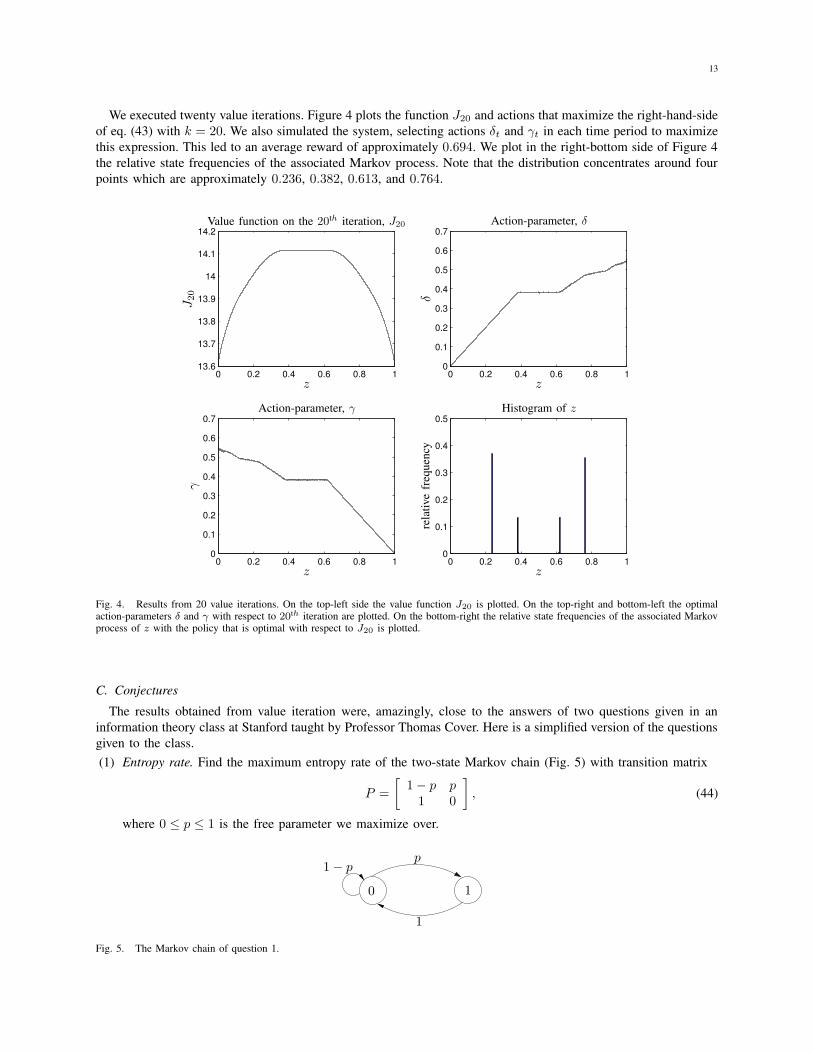
We executed twenty value iterations. Figure 4 plots the function J20 and actions that maximize the right-hand-sideof eq. (43) with k = 20. We also simulated the system, selecting actions δt and γt in each time period to maximizethis expression. This led to an average reward of approximately 0.694. We plot in the right-bottom side of Figure 4the relative state frequencies of the associated Markov process. Note that the distribution concentrates around fourpoints which are approximately 0.236, 0.382, 0.613, and 0.764.
0 0.2 0.4 0.6 0.8 113.6
13.7
13.8
13.9
14
14.1
14.2
0 0.2 0.4 0.6 0.8 10
0.1
0.2
0.3
0.4
0.5
0.6
0.7
0 0.2 0.4 0.6 0.8 10
0.1
0.2
0.3
0.4
0.5
0.6
0.7
0 0.2 0.4 0.6 0.8 10
0.1
0.2
0.3
0.4
0.5PSfrag replacements
rela
tive
freq
uenc
y
Value function on the 20th iteration, J20
J20
Action-parameter, δ
Action-parameter, γ Histogram of z
δ
γ
zz
zz
Fig. 4. Results from 20 value iterations. On the top-left side the value function J20 is plotted. On the top-right and bottom-left the optimalaction-parameters δ and γ with respect to 20th iteration are plotted. On the bottom-right the relative state frequencies of the associated Markovprocess of z with the policy that is optimal with respect to J20 is plotted.
C. Conjectures
The results obtained from value iteration were, amazingly, close to the answers of two questions given in aninformation theory class at Stanford taught by Professor Thomas Cover. Here is a simplified version of the questionsgiven to the class.(1) Entropy rate. Find the maximum entropy rate of the two-state Markov chain (Fig. 5) with transition matrix
P =
[1− p p
1 0
], (44)
where 0 ≤ p ≤ 1 is the free parameter we maximize over.PSfrag replacements
p1− p
1
0 1
Fig. 5. The Markov chain of question 1.
14
(2) Number of sequences. To first order in the exponent, what is the number of binary sequences of length nwith no two 1’s in a row?
The entropy rate of the Markov chain of question (1) is given by H(p)1+p , and when maximizing over 0 ≤ p ≤ 1,
we get that p = 3−√
52 and the entropy rate is 0.6942. It can be shown that the number of sequences of length
n − 1 that do not have two 1’s in a row is the nth number in the Fibonacci sequence. This can be proved byinduction in the following way. Let us denote (N 0
n, N1n) the number of sequences of length n with the condition
of not having two 1’s in a row that are ending with ‘0’ and with ‘1’ respectively. For the sequences that end with‘0’ we can either add a next bit ‘1’ or ‘0’ and for the sequences that end with ‘1’ we can add only ‘0’. HenceN0n+1 = N0
n +N1n and N1
n+1 = N0n. By repeating this logic, we get that N 0
n behaves as a Fibonacci sequence. Tofirst order in the exponent, the Fibonacci number behaves as limn→∞ 1
n log fn = log 1+√
52 = 0.6942, where the
number, 1+√
52 , is called the golden ratio. The golden ratio is also known to be a positive number that solves the
equation 1φ = 1− φ, and it appears in many math, science and art problems [27]. As these problems illustrate, the
number of typical sequences created by the Markov process given in question (1) is, to first order in the exponent,equal to the number of binary sequences that do not have two 1’s in a row.
Let us consider a policy for the dynamic program associated with a binary random process that is created bythe Markov chain from question 1 (see Fig 5). Let the state of the Markov process indicate if the input to thechannel will be the same or different from the state of the channel. In other words, if at time t the binary Markovsequence is ‘0’ then the input to the channel is equal to the state of the channel, i.e. xt = st−1. Otherwise, theinput to the channel is a complement to the state of the channel, i.e. xt = st−1 ⊕ 1. This scheme uniquely definesthe distribution p(xt|st−1, y
t−1):
p(Xt = st−1|st−1, yt−1) =
{1− p if st−1 = yt−1,1 if st−1 6= yt−1.
(45)
This distribution is derived from the fact that for the trapdoor channel the state evolves according to equation (3)which can be written as
st−1 ⊕ yt−1 = xt−1 ⊕ st−2. (46)
Hence, if st−1 6= yt−1 then necessarily also xt−1 6= st−2. This means that the tuple (st−1, yt−1) defines the state ofthe Markov chain at time t− 1 and the tuple (xt, st−1) defines the state of the Markov chain at time t. Having thedistribution p(xt|st−1, y
t−1), for the following four values of z, {b1 ,√
5−2, b2 , 3−√
52 , b3 ,
√5−12 , b4 , 3−
√5},
the corresponding actions γ(z) and δ(z) which are defined in eq. (40,41) are:
z γ(z) δ(z)
b1 or b2√
5−12 (1− z) z
b3 or b4 1− z√
5−12 z
It can be verified, by using eq. (35), that the only values of z ever reached are,
z ∈{b1 ,
√5− 2, b2 ,
3−√
5
2, b3 ,
√5− 1
2, b4 , 3−
√5
}, (47)
and the transitions are a function of yt shown graphically in Figure 6. Our goal is to prove that an extension ofthis policy is indeed optimal. Based on the result of Question 1, we conjugate that the entropy rate of the averagereward is
ρ =H( 3−
√5
2 )
1 + 3−√
52
= log
√5 + 1
2≈ 0.6942. (48)
It is interesting to notice that all the numbers appearing above can be written in terms of the golden ratio, φ =√
5−12 .
In particular, ρ = log φ, b1 = 2φ− 3, b2 = 2− φ, b3 = φ− 1 and b4 = 4− 2φ.
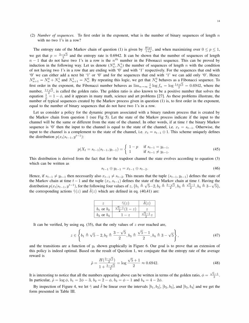
By inspection of Figure 4, we let γ and δ be linear over the intervals [b1, b2], [b2, b3], and [b3, b4] and we get theform presented in Table III.

15
PSfrag replacements
111
10
000
b1b1
b2b2
b3b3
b4b4
βt−1 βtyt
Fig. 6. The transition between βt−1 and βt, under the policy δ, γ.
z γ(z) δ(z)
b1 ≤ z ≤ b2√
5−12 (1− z) z
b2 ≤ z ≤ b3 3−√
52
3−√
52
b3 ≤ z ≤ b4 1− z√
5−12 z
TABLE IIICONJECTURED POLICY WHICH IN THE NEXT SECTION WILL BE PROVEN TO BE TRUE.
We now propose differential values h(z) for z ∈ [b1, b4]. If we assume that δ and γ maximize the right-hand-sideof the Bellman equation (eq. 34) for z ∈ [b1, b4] with h = h and ρ = ρ, we obtain
h(z) = H
(1
2
)− (√
5− 2)− ρ+ h(3−√
5), b2 ≤ z ≤ b3, (49)
h(z) = H
(√5 + 1
4z
)−3−
√5
2z−ρ+
√5 + 1
4zh(3−
√5)+
(1−√
5 + 1
4z
)h
(1− z
1−√
5+14 z
), b3 ≤ z ≤ b4.
(50)The equation for the range b1 ≤ z ≤ b2 is implied by the symmetry relation: h(z) = h(1− z).
If a scalar ρ and function h solve Bellman’s equation, so do ρ and h + c1 for any scalar c. Therefore, there isno loss of generality in setting h(1/2) = 1. From eq. (49) we have that
h(z) = 1, b2 ≤ z ≤ b3. (51)
In addition, by symmetry considerations we can deduce that h(√
5− 2) = h(3−√
5) and from eq. (49) we obtain
h(√
5− 2) = h(3−√
5) = ρ− 2 +√
5 ≈ 0.9303. (52)
Taking symmetry into consideration and applying eq. (50) twice we obtain,
h(z) = H(z) + ρz + c1, b3 ≤ z ≤ b4, (53)
where c1 = log(3−√
5). By symmetry we obtain
h(z) = H(z)− ρz + c2, b1 ≤ z ≤ b2. (54)
where c2 = log(√
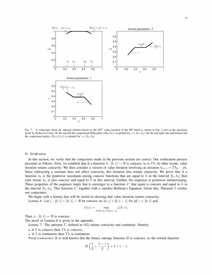
5− 1)The conjectured policy (γ, δ), which is given in Table III, and the conjectured differential value h, which is given
in eq. (51)-(54), are plotted in Fig. 7.
16
0 0.2 0.4 0.6 0.8 10
0.1
0.2
0.3
0.4
0.5
0.6
0 0.2 0.4 0.6 0.8 10
0.1
0.2
0.3
0.4
0.5
0.6
0 0.2 0.4 0.6 0.8 10
0.2
0.4
0.6
0.8
1
PSfrag replacements
1− z −→
3−√
52
√5−12 (1− z)↓
←− z
3−√
52 ↖
√5−12 z
H(z)− ρz + c2↘
H(z) + ρz + c1↙
b1↓
b2↓
b3↓
b4↓
h
Action-parameter, δ
Action-parameter, γ
δ
γ
z
z
Fig. 7. A conjecture about the optimal solution based on the 20th value iteration of the DP which is shown in Fig. 4 and on the questionsgiven by Professor Cover. On the top-left the conjectured differential value h(z) is plotted for z ∈ [b1, b4]. On the top-right side and bottom-leftthe conjectured policy (δ(z),γ(z)) is plotted for z ∈ [b1, b4]
D. Verification
In this section, we verify that the conjectures made in the previous section are correct. Our verification processproceeds as follows. First, we establish that if a function h : [0, 1] 7→ < is concave, so is Th. In other words, valueiteration retains concavity. We then consider a version of value iteration involving an iteration hk+1 = Thk − ρ1.Since subtracting a constant does not affect concavity, this iteration also retains concavity. We prove that if afunction h0 is the pointwise maximum among concave functions that are equal to h in the interval [b1, b4] theneach iterate hk is also concave and equal to h in this interval. Further, the sequence is pointwise nonincreasing.These properties of the sequence imply that it converges to a function h∗ that again is concave and equal to h inthe interval [b1, b4]. This function h∗ together with ρ satisfies Bellman’s Equation. Given this, Theorem 5 verifiesour conjectures.
We begin with a lemma that will be useful in showing that value iteration retains concavity.Lemma 6: Let ζ : [0, 1]× [0, 1] 7→ < be concave on [0, z]× [0, 1− z] for all z ∈ [0, 1] and
ψ(z) = supδ∈[0,z],γ∈[0,1−z]
ζ(δ, γ).
Then ψ : [0, 1] 7→ < is concave.The proof of Lemma 6 is given in the appendix.
Lemma 7: The operator T , defined in (42) retains concavity and continuity. Namely,• if h is concave then Th is concave,• if h is continuous then Th is continuous.Proof (concavity): It is well-known that the binary entropy function H is concave, so the reward function
H
(1
2+δ − γ
2
)+ δ + γ − 1
17
is concave in (δ, γ).
Next, we show that if h(z) is concave then 1+δ−γ2 h
(2δ
1+δ−γ
)is concave in (δ, γ). Let ξ1 = 1+δ1−γ1
2 and
ξ2 = 1+δ2−γ2
2 . We will show that, for any α ∈ (0, 1),
αξ1h
(δ1ξ1
)+ (1− α)ξ2h
(δ2ξ2
)≥ (αξ1 + (1− α)ξ2)h
(αδ1 + (1− α)δ2
αξ1 + (1− α)ξ2
). (55)
Dividing both sides by (αξ1 + (1− α)ξ2) we get
αξ1αξ1 + (1− αξ2)
h
(δ1ξ1
)+
(1− α)ξ2αξ1 + (1− αξ2)
h
(δ2ξ2
)≥ h
(αδ1 + (1− α)δ2
αξ1 + (1− α)ξ2
). (56)
Note that the last inequality is true because of the concavity of h. It follows that
f(δ, γ) , H(
1
2+δ − γ
2
)+ δ + γ − 1 +
1 + δ − γ2
h
(2δ
1 + δ − γ
)+
1− δ + γ
2h
(1− 2γ
1− δ + γ
)(57)
is concave in (δ, γ). Since(Th)(z) = sup
δ∈[0,z],γ∈[0,1−z]f(δ, γ),
it is concave by Lemma 6.
Proof (continuity): Note that the binary entropy function H is continuous. Further, h(
2δ1+δ−γ
)and
h(
1− 2γ1−δ+γ
), are continuous over the region {(δ, γ)|δ ≥ 0, γ ≥ 0, δ + γ ≤ 1}. It follows that f(δ, γ) is
continuous over the region {(δ, γ)|δ ≥ 0, γ ≥ 0, δ + γ ≤ 1}. Hence,
(Th)(z) = supδ∈[0,z],γ∈[0,1−z]
f(δ, γ)
is continuous over [0, 1].
Let us construct value iteration function hk(z) as follows. Let h0(z) be the pointwise maximum among concavefunctions satisfying h0(z) = h(z) for z ∈ [b1, b4], where h(z) is defined in eq.(51)-(54). Note that h0(z) is concaveand that for z /∈ [b1, b4], h(z) is a linear extrapolation from the boundary of [b1, b4]. Let
hk+1(z) = (Thk)(z)− ρ, (58)
andh∗(z) , lim sup
k→∞hk(z). (59)
The following lemma shows several properties of the sequence of function hk(z) including the uniformconvergence. The uniform convergence is needed for verifying the conjecture, while the other properties areintermediate steps in proving the uniform convergence.
Lemma 8: The following properties hold:
8.1 for all k ≥ 0, hk(z) is concave and continuous in z8.2 for all k ≥ 0, hk(z) is symmetric around 1
2 , i.e.
hk(z) = hk(1− z) (60)
8.3 for all k ≥ 0, hk(z) is fixed point for z ∈ [b1, b4], i.e.,
hk(z) = h(z), z ∈ [b1, b4], (61)
and the stationary policy µ(z) = (δ(z), γ(z)), where (δ(z), γ(z)) are defined in Table III, satisfies (Tµhk)(z) =(Thk)(z)
8.4 hk(z) is uniformly bounded in k and z, i.e.,
supk
supz∈[0,1]
|hk(z)| <∞ (62)
18
8.5 hk(z) is monotonically nonincreasing in k, i.e.
limk→∞
hk(z) = h∗(z) (63)
8.6 hk(z) converges uniformly to h∗(z)
Proof of 8.1: Since h0(z) is concave and continuous and since the operator T retain continuity and concavity(see Lemma 7),it follows that hk(z) is concave and continuous for every k.
Proof of 8.2: We prove this property by induction. First notice that h0(z) is symmetric and satisfies h0(z) =h0(1− z). Now let us show that if it holds for hk then it holds for hk+1.
Let fk(δ, γ) denote the expression maximized to obtain (Thk)(z), i.e.
fk(δ, γ) , H(
1
2+δ − γ
2
)+ δ + γ − 1 +
1 + δ − γ2
hk
(2δ
1 + δ − γ
)+
1− δ + γ
2hk
(1− 2γ
1− δ + γ
). (64)
Notice that fk(δ, γ) = fk(γ, δ). Also observe that replacing the argument z with 1−z in Thk yield the same resultas exchanging between γ and δ. From those two observations follows that Thk(z) = Thk(1 − z) and from thedefinition of hk+1 given in (58) follows that hk+1(z) = hk+1(1− z).
Proof of 8.3: We prove this property by induction. Notice that h0 satisfies h0(z) = h(z) for z ∈ [b1, b4]. Weassume that hk satisfies hk(z) = h(z) and then we will prove the property for hk+1. We will show later in thisproof that for z ∈ [b1, b4],
(Tµhk)(z) = (Thk)(z). (65)
Since (Tµhk)(z)− ρ = h(z) for all z ∈ [b1, b4] (see eq.49-54 ) it follows that hk+1(z) = h(z) for all z ∈ [b1, b4].Now, let us show that (65) holds. Recall that in the proof of Lemma 7, eq. (64), we showed that fk(δ, γ) is
concave in (δ, γ). The derivative with respect to δ is,
∂fk(δ, γ)
∂δ=
1
2log
1− δ + γ
1 + δ − γ + 1 +1
2hk
(2δ
1 + δ − γ
)− 1
2hk
(2γ
1− δ + γ
)
+1− γ
1 + δ − γ h′k
(2δ
1 + δ − γ
)+
γ
1− δ + γh′k
(2γ
1− δ + γ
). (66)
The derivative with respect to γ is entirely analogous and can be obtained by mutually exchanging γ and δ.For z ∈ [b2, b3], the action γ(z) = δ(z) = 3−
√5
2 is feasible and 2γ(z)
1−δ(z)+γ(z)= 2δ(z)
1+δ(z)−γ(z)= b4. Moreover, it
is straightforward to check that the derivatives of fk are zero at (γ(z), δ(z)), and since fk is concave, (γ(z), δ(z))attains the maximum. Hence, (Tµh)(z) = (Th)(z) for z ∈ [b2, b3].
For z ∈ [b3, b4], γ(z) = 1− z and δ(z) =√
5−12 z. Note that 2γ(z)
1−δ(z)+γ(z)and 2δ(z)
1+δ(z)−γ(z)are in [b1, b2]∪ [b3, b4].
Using expressions for h(z) given in equations (53) and (54), we can write derivatives of f at (δ(z), γ(z)) as
∂f(δ(z), γ(z))
∂δ= log
1− δ(z)− γ(z)
2δ(z)+ 1 + ρ = 0, (67)
∂f(δ(z), γ(z))
∂γ= log
1− δ(z)− γ(z)
2γ(z)+ 1 + ρ ≥ 0. (68)
Notice that γ(z) is the maximum of the feasible set [0, 1−z] and the derivative of fk with respect to γ at (δ(z), γ(z))is positive. In addition, δ(z) is in the interior of the feasible set [0, z] and the derivative of fk with respect to δ at(δ(z), γ(z)) is zero. Since fk is concave, any feasible change in (γ(z), δ(z)) will decrease the value of the function.Hence, (Tµhk)(z) = (Thk)(z) for z ∈ [b3, b4]. The situation for z ∈ [b1, b2] is completely analogous.
Proof of 8.4: From Propositions 8.1- 8.3, it follows that the maximum over z of hk(z) is attained at z = 1/2and hk(1/2) = 1 for all k. Further more because of concavity and symmetry the minimumm of hk(z) is attainedat z = 0 and z = 1. Hence it is enough to show that hk(0) is uniformly bounded from below for all k.
For z = 0 let us consider the action γ = 1−b21−b2 and δ = 0 and for b1 ≤ z ≤ b4 the action γ(z), δ(z). Now let us
prove that under this policy hk(0) that is less or equal the optimal value is uniformly bounded.Under this policy hk+1(0) = (Thk)(0)− ρ becomes
hk(0) = c+ αhk−1(0) + (1− α)1− ρ (69)
19
where c and α are constant: c = H(
11+b2
)+ b2 − 1 , α = 1−b2
2 .Iterating the equation (69) k − 1 time we get
hk(0) = (c+ 1− α− ρ)k−1∑
i=0
αi + αkh0(0). (70)
Since α < 1, hk(0) is uniformly bounded for all k.Proof of 8.5: By Proposition 8.1 hk is concave for each k and by Proposition 8.3 hk(z) = h(z) for z ∈ [b1, b4].
Since h0 is the pointwise maximum of functions satisfying this condition, we must have h0 ≥ h1. It is easy tosee that T is a monotonic operator. As such, hk ≥ hk+1 for all k. Proposition 8.4 establishes that the sequence isbounded below, and therefore it converges pointwise.
Proof of 8.6: By Proposition 8.1, each hk is concave and continuous. Further, by Proposition 8.5, the sequencehas a pointwise limit h∗ which is concave. Concavity of h∗ implies continuity [28, Theorem 10.1] over (0, 1). Leth† be the continuous extension of h∗ from (0, 1) to [0, 1]. Since h∗ is concave, h† ≥ h∗.
By Proposition 8.5 , hk ≥ h∗. It follows from continuity of hk that hk ≥ h†. Hence, h∗(z) = limk hk(z) ≥ h†(z)for z ∈ [0, 1]. Recalling that h∗ ≤ h†, we have h∗ = h†.
Since the iterates hk are continuous and monotonically nonincreasing and their pointwise limit h∗ is continuous,hk converges uniformly by Dini’s Theorem [29].
The following theorem verifies our conjectures.Theorem 9: The function h∗ and scalar ρ satisfy ρ1 + h∗ = Th∗. Further, ρ is the optimal average reward and
there is an optimal policy that takes actions δt = δ(zt−1) and γt = γ(zt−1) whenever zt−1 ∈ [b1, b4].Proof: Since the sequence hk+1 = Thk − ρ1 converges uniformly and T is sup-norm continuous, h∗ =
Th∗ − ρ1. It follows from Theorem 5 that ρ is the optimal average reward. Together with Proposition 8.3, thisimplies existence of an optimal policy that takes actions δt = δ(zt−1) and γt = γ(zt−1) whenever zt−1 ∈ [b1, b4].
VII. A CAPACITY-ACHIEVING SCHEME
In this section we describe a simple encoder and decoder pair that provides error-free communication through thetrapdoor channel with feedback and known initial state. We then show that the rates achievable with this encodingscheme are arbitrarily close to capacity.
It will be helpful to discuss the input and output of the channel in different terms. Recall that the state of thechannel is known to the transmitter because it is a deterministic function of the previous state, input, and output,and the initial state is known. Let the input action, x, be one of the following:
x =
{0, input ball is same as state1, input ball is opposite of state
Also let the output be recorded differentially as,
y =
{0, received ball is same as previous1, received ball is opposite of previous
where y1 is undefined and irrelevant for our scheme.
A. Encode/Decode Scheme
Encoding. Each message is mapped to a unique binary sequence of N actions, xn, that ends with 0 and has nooccurrences of two 1’s in a row. The input to the channel is derived from the action and the state as, xk = xk⊕sk−1.
Decoding. The channel outputs are recorded differentially as, yk = yk ⊕ yk−1, for k = 2, ..., N . Decoding of theaction sequence is accomplished in reverse order, beginning with xN = 0 by construction.
Lemma 10: If xk+1 is known to the decoder, xk can be correctly decoded.Proof: Table IV shows how to decode xk from xk+1 and yk+1.
Proof of case 1. Assume that xk = 1. At time k, just before the output is received, there are balls of both typesin the channel. By symmetry we can assume that the ball that exits is labeled ‘0.’ Therefore, the ball labeled ‘1’remains in the channel. According to the encoding scheme, xk+1 = 0 because repeated 1’s are not allowed, which

20
TABLE IVDECODING THE INPUT FROM THE NEXT OUTPUT AND INPUT.
yk+1 xk+1 xkCase 1 0 - 0Case 2 - 1 0Case 3 1 0 1
means the input to the channel at time k is labeled ‘1.’ It is clear that the ball that comes out of the channel attime k + 1 must be labeled ‘1.’ This leads to the contradiction, yk+1 = 1.
Proof of case 2. By construction there are never two 1’s in a row.Proof of case 3. Assume that xk = 0. The balls that enter the channel both at times k and k + 1 are the same
type as the ball that is in the channel, therefore that same type of ball must come out each of the two times. Thisleads to the contradiction, yk+1 = 0.
Decoding example. Table V shows an example of decoding a sequence of actions for N = 10.
TABLE VDECODING EXAMPLE
Variable Value Reasonyn 1011010001 Channel outputyn *110111001 Differential outputxn 0 Given
10 Case 3010 Case 1 or 2
0010 Case 110010 Case 3
010010 Case 21010010 Case 3
01010010 Case 1 or 2101010010 Case 3
0101010010 Case 2
B. Rate
Under this encoding scheme, the number of admissible unique action sequences is the number of binary sequencesof length N − 1 without any repeating 1’s. This is known to be exponentially equivalent to φN−1, where φ is thegolden ratio (see question 2 in section VI-C). Since limN→∞ N−1
N log φ = log φ, rates arbitrary close to log φ areachievable.
C. Remarks
Early decoding. Decoding can often begin before the entire block is received. Table IV shows us that we candecode xk without knowledge of xk+1 for any k such that yk+1 = 0. Decoding can begin from any such pointand work backward.
Preparing the channel. This communication scheme can still be implemented even if the initial state of the channelis not known as long as some channel uses are expended to prepare the channel for communication. The repeatingsequence 010101... can be used to flush the channel until the state becomes evident. As soon as the output of the

21
channel is different from the input, both the transmitter (through feedback) and the receiver know that the state isthe previous input. At that point, zero-error communication can begin as described above.
This flushing method requires a random and unbounded number of channel uses. However, it only needs tobe performed once after which multiple blocks of communication can be accomplished. The expected numberof required channel uses is easily found to be 3.5, since the number of uses is geometrically distributed whenconditioned on the initial state.
Permuting relay channel similarity. The permuting relay channel described in [3] has the same capacity as thetrapdoor channel with feedback. A connection can be made using the achievable scheme described in this section.
The permuting relay channel supposes that the transmitter chooses an input distribution to the channel that isindependent of the message to be sent. The transmitter lives inside the trapdoor channel and chooses which of thetwo balls will be released to the receiver in order to send the message. Without proof here, let us assume that thedeterministic input 010101... is optimal. Now we count how many distinguishable outputs are possible.
It is helpful to view this as a permutation channel as described in section II where the permuting is not donerandomly but deliberately. Notice that for this input sequence, after each time that a pair of different numbersis permuted, the next pair of numbers will be the same, and the associated action will have no consequence.Therefore, the number of distinguishable permutations can be easily shown to be related to the number of uniquebinary sequences without two 1’s in a row.
Three channels have same feedback capacity. The achievable scheme in this section allows zero-error communi-cation. Therefore, this scheme could also be used to communicate with feedback through the permuting jammerchannel from [3], which assumes that the trapdoor channel behavior is not random but is the worst possible tomake communication difficult.
In the permuting relay channel [3], all information (input and output) is available to the transmitter, so feedbackis irrelevant. Thus we find that the feedback capacity (with known initial state) is the same for the trapdoor,permuting jammer, and permuting relay channels.
Constrained coding. The capacity-achieving scheme requires uniquely mapping a message to a sequence with theconstraint of having no two 1’s in a row. A practical way of accomplishing this can be done by using a techniquecalled enumeration [30]. The technique translates the message into codewords and vice versa by invoking analgorithmic procedure rather then using a lookup table. Vast literature on coding a source word into a constrainedsequence can be found in [31] and [32].
VIII. CONCLUSION AND FURTHER WORK
This paper gives an information theory formulation for the feedback capacity of a strongly connected unifilarfinite state channel and it shows that the feedback capacity expression can be formulated as an average-rewarddynamic program. For the trapdoor channel, we were able to solve explicitly the dynamic programming problemand to show that the capacity of the channel is the log of the golden ratio. Furthermore, we were able to find asimple encoding/decoding scheme that achieves this capacity.
There are several directions in which this work can be extended.• Generalization: Extend the trapdoor channel definition. It is possible to add parameters to the channel and
make it more general. For instance, there could be a parameter that determines which ball from the two hasthe higher probability of being the output of the channel. Other parameters might include the number of ballsthat can be in the channel at the same time or the number of different types of balls that are used. These tiein nicely with viewing the trapdoor channel as a chemical channel.
• Unifilar FSC Problems: Find strongly connected unifilar FSC’s that can be solved, similar to the way wesolved the trapdoor channel.
• Dynamic Programming: Classify a family of average-reward dynamic programs that have analytic solutions.
ACKNOWLEDGMENT
The authors would like to thank Tom Cover, who introduced the trapdoor channel to H. Permuter and P. Cuff andasked them the two questions that appear in subsection VI-C, which eventually led to the solution of the dynamicprogramming and to the simple scheme that achieves the feedback capacity.
22
REFERENCES
[1] D. Blackwell. Information theory. Modern mathematics for the engineer: Second series, pages 183–193, 1961.[2] R. Ash. Information Theory. Wiley, New York, 1965.[3] R. Ahlswede and A. Kaspi. Optimal coding strategies for certain permuting channels. IEEE Trans. Inform. Theory, 33(3):310–314, 1987.[4] R. Ahlswede, N. Cai, and Z. Zhang. Zero-error capacity for models with memory and the enlightened dictator channel. IEEE Trans.
Inform. Theory, 44(3):1250–1252, 1998.[5] K. Kobayashi and H. Morita. An input/output recursion for the trapdoor channel. In Proceedings ISIT2002, page 423. IEEE, 2002.[6] K. Kobayashi. Combinatorial structure and capacity of the permuting relay channel. IEEE Trans. on Inform. Theory, 33(6):813–826, Nov.
1987.[7] P. Piret. Two results on the permuting mailbox channel. IEEE Trans. Inform. Theory, 35:888–892, 1989.[8] W. K. Chan. Coding strategies for the permuting jammer channel. In Proceedings ISIT2000, page 211. IEEE, 1993.[9] S.C. Tatikonda. Control under communication constraints. Ph.D. disertation, MIT, Cambridge, MA, 2000.
[10] S Tatikonda S Yang, A Kavcic. Feedback capacity of finite-state machine channels. IEEE Trans. Inform. Theory, pages 799–810, 2005.[11] J. Chen and T. Berger. The capacity of finite-state Markov channels with feedback. IEEE Trans. on Information theory, 51:780–789, 2005.[12] S. Tatikonda and S. Mitter. The capacity of channels with feedback. September 2006.[13] D. P. Bertsekas. Dynamic Programming and Optimal Control: Vols 1 and 2. AthenaScientific, Belmont, MA., 2005.[14] A. Arapostathis, V. S. Borkar, E. Fernandez-Gaucherand, M. K. Ghosh, and S. Marcus. Discrete time controlled Markov processes with
average cost criterion - a survey. SIAM Journal of Control and Optimization, 31(2):282–344, 1993.[15] J. Ziv. Universal decoding for finite-state channels. IEEE Trans. Inform. Theory, 31(4):453–460, 1985.[16] T. W. Benjamin. Coding for a noisy channel with permutation errors”. Ph.d. dissertation, Cornel Univ., Ithaca, NY, 1975.[17] H. H. Permuter, T. Weissman, and A. J. Goldsmith. Capacity of finite-state channels with time-invariant deterministic feedback. In
Proceedings ISIT2006. IEEE, 2006.[18] H. H. Permuter, T. Weissman, and A. J. Goldsmith. Finite state channels with time-invariant deterministic feedback. Submitted to IEEE
Trans. Inform. Theory. Availble at arxiv.org/pdf/cs.IT/0608070, Sep 2006.[19] S.S. Pradhan. Source coding with feedforward: Gaussian sources. In Proceedings 2004 International Symposium on Information Theory,
page 212, 2004.[20] R. Venkataramanan and S. S. Pradhan. Source coding with feedforward: Rate-distortion function for general sources. In IEEE Information
theory workshop (ITW), 2004.[21] R. Zamir, Y. Kochman, and U. Erez. Achieving the gaussian rate-distortion function by prediction. Submitted for publication in “IEEE
Trans. Inform. Theory”, July 2006.[22] G. Kramer. Capacity results for the discrete memoryless network. IEEE Trans. Inform. Theory, 49:4–21, 2003.[23] G. Kramer. Directed Information for Channels with Feedback. Ph.d. dissertation, Swiss Federal Institute of Technology Zurich, 1998.[24] A. Rao, A.O. Hero, D.J. States, and J.D. Engel. Inference of biologically relevant gene influence networks using the directed information
criterion. In ICASSP 2006 Proceedings, 2006.[25] J. Massey. Causality, feedback and dircted information. Proc. Int. Symp. Information Theory Application (ISITA-90), pages 303–305, 1990.[26] Q. Zhu and X. Guo. Value iteration for average cost Markov decision processes in Borel spaces. AMRX Applied Mathematics Research
eXpress, 2:61–76, 2005.[27] L. Mario. The golden ratio : the story of phi, the world’s most astonishing number. Broadway Books, New York, 2002.[28] R. T. Rockafellar. Convex Analysis. Princeton Univ. Press, New Jersey, 1970.[29] Jerrold E. Marsden and Michael J. Hoffman. Elementary Classical Analysis. W. H. Freeman and Company, New York, NY, 2nd edition,
1993.[30] T. M. Cover. Enumerative source encoding. IEEE Trans. Inform. Theory, 19:73–77, 1973.[31] B.H. Marcus, R.M. Roth, and P.H. Siegel. Constrained systems and coding for recording channels. In V.S. Pless and W.C.Hu, editors, In
Handbook of Coding Theory, Amsterdam, 1998. Elsevier.[32] K.A.S. Immink. Codes for Mass Data Storage Systems. Shannon Foundation, Rotterdam, The Netherlands, 2004.
APPENDIX
Proof of Lemma 6: For any z1, z2 ∈ [0, 1] and θ ∈ (0, 1),
ψ(θz1 + (1− θ)z2) = supδ∈[0,θz1+(1−θ)z2]
supγ∈[0,1−(θz1+(1−θ)z2)]
ζ(δ, γ)
= supδ1∈[0,θz1]
supδ2∈[0,(1−θ)z2]
supγ1∈[0,θ(1−z1)]
supγ2∈[0,(1−θ)(1−z2)]
ζ(δ1 + δ2, γ1 + γ2)
(a)= sup
δ′1∈[0,z1]
supδ′2∈[0,z2]
supγ′1∈[0,1−z1]
supγ′2∈[0,1−z2]
ζ(θδ′1 + (1− θ)δ′2, θγ′1 + (1− θ)γ′2)
(b)
≥ supδ′1∈[0,z1]
supδ′2∈[0,z2]
supγ′1∈[0,1−z1]
supγ′2∈[0,1−z2]
θζ(δ′1, γ′1) + (1− θ)ζ(δ′2, γ
′2)
= supδ′1∈[0,z1]
supγ′1∈[0,1−z1]
θζ(δ′1, γ′1) + sup
δ′2∈[0,z2]
supγ′2∈[0,1−z2]
(1− θ)ζ(δ′2, γ′2)
= θψ(z1) + (1− θ)ψ(z2). (71)
Step (a) is a change of variable (θδ′1 = δ1, (1− θ)δ′2 = δ2, θγ′1 = γ1, (1− θ)γ′2 = γ2). Step (b) is due to concavity
of ζ.