1

Calculating Polynomials

• We will use a generic polynomial form of:

where the coefficient values are known constants

• The value of x will be the input and the result is the value of the polynomial using this x value

011

1 )(p axaxaxax nn

nn

2

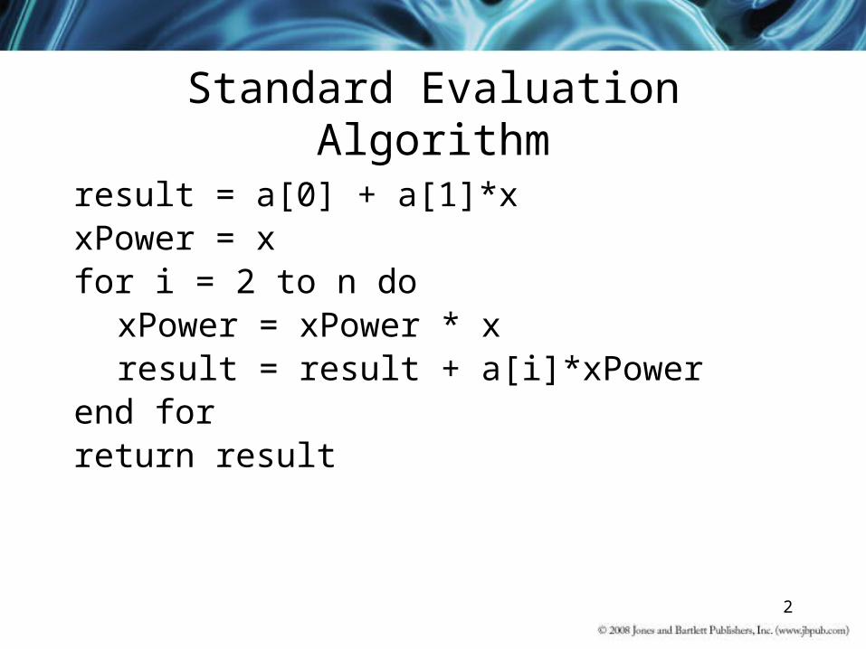
Standard Evaluation Algorithm

result = a[0] + a[1]*xxPower = xfor i = 2 to n do

xPower = xPower * xresult = result + a[i]*xPower

end forreturn result

3

Analysis

• Before the loop, there is– One multiplication– One addition

• The for loop is done N-1 times– There are two multiplications in the loop– There is one addition in the loop

• There are a total of– 2N – 1 multiplications– N additions

4

Horner’s Method

• Based on the factorization of a polynomial• The generic equation is factored as:

• For example, the equation:

• would be factored as:

475 )(p 23 xxxx

5

Horner’s Method Algorithm

result = a[n]

for i = n - 1 down to 0 doresult = result * xresult = result + a[i]

end forreturn result

6

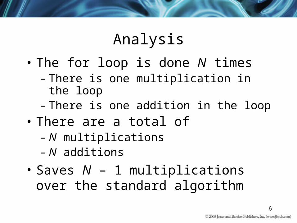
Analysis

• The for loop is done N times– There is one multiplication in the loop– There is one addition in the loop

• There are a total of– N multiplications– N additions

• Saves N – 1 multiplications over the standard algorithm

7

Preprocessed Coefficients

• Uses a factorization of a polynomial based on polynomials of about half the original polynomial’s degree

• For example, where the standard algorithm would do 255 multiplications to calculate x256, we could square x and then square the result seven more times to get the same result

8

Preprocessed Coefficients

• Used with polynomials that are monic (an=1) and have a highest power that is one less than a power of 2

• If the polynomial has highest power that is 2k – 1, we can factor it as:

where j = 2k-1

)()(q* )(p xrxbxx j

9

Preprocessed Coefficients

• If we choose b so that it is aj-1 – 1, q(x) and r(x) will both be monic, and so the process can be recursively applied to them as well

10

Preprocessed Coefficients Example

• For the example equation of:

because the highest degree is 3 = 22 –1, j would be 21 = 2, and b would have a value of a1 – 1 = 6

• This makes one factor x2 + 6, and we divide p(x) by this polynomial to find q(x) and r(x)

475 )(p 23 xxxx

11

Preprocessed Coefficients Example

• The division is:

which gives

5

26

3065

4756

23

232

x

x

xxx

xxxx

265*6 )(p 2

xxxx

12

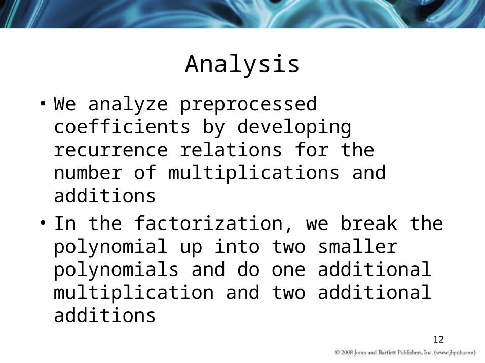
Analysis

• We analyze preprocessed coefficients by developing recurrence relations for the number of multiplications and additions

• In the factorization, we break the polynomial up into two smaller polynomials and do one additional multiplication and two additional additions

13

Analysis

• Because we required that N = 2k – 1, we get:

M(1) = 0 A(1) = 0M(k) = 2M(k–1) + 1 A(k) = 2A(k–1) + 2

• Solving these equations gives about N/2 multiplications and (3N – 1)/2 additions

• We need to include the k – 1 (or lg N) multiplications needed to calculate the series of values x2, x4, x8, …

14

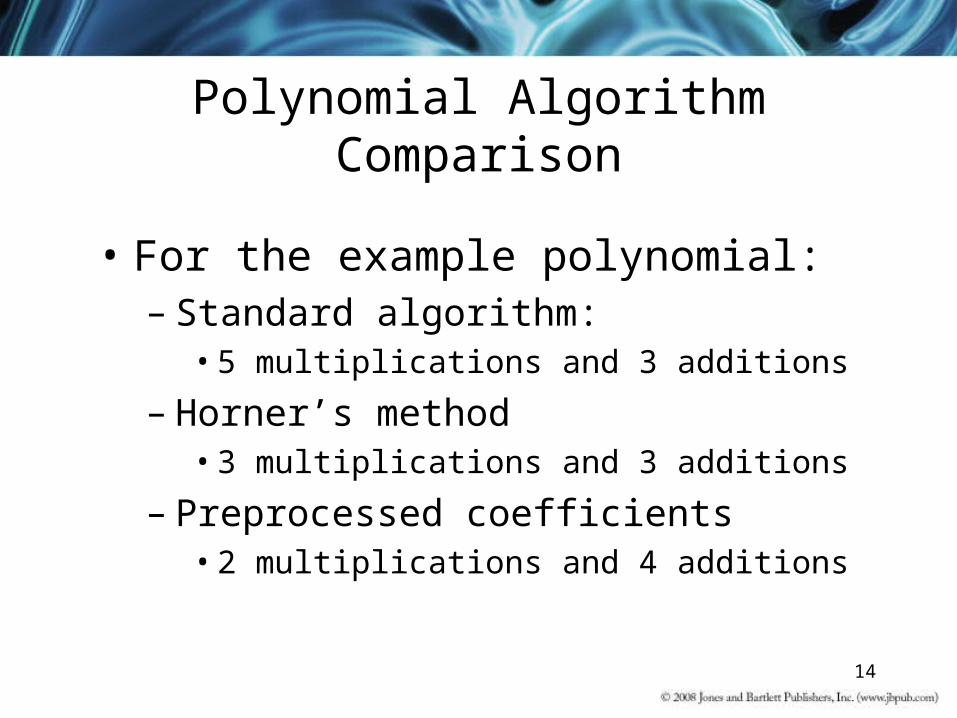
Polynomial Algorithm Comparison

• For the example polynomial:– Standard algorithm:

• 5 multiplications and 3 additions

– Horner’s method• 3 multiplications and 3 additions

– Preprocessed coefficients• 2 multiplications and 4 additions

15

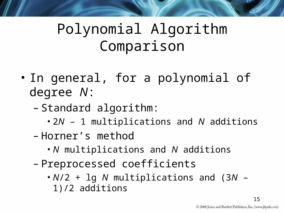
Polynomial Algorithm Comparison

• In general, for a polynomial of degree N:– Standard algorithm:

• 2N – 1 multiplications and N additions

– Horner’s method• N multiplications and N additions

– Preprocessed coefficients• N/2 + lg N multiplications and (3N – 1)/2 additions

16

Linear Equations

• A system of linear equations is a set of N equations in N unknowns:

a11x1 + a12x2 + a13x3 + … + a1NxN = b1

a21x1 + a22x2 + aa3x3 + … + a2NxN = b2

aNx1 + aN2x2 + aN3x3 + … + aNNxN = bN

17

Linear Equations

• When these equations are used, the coefficients (a values) are constants and the results (b values) are typically input values

• We want to determine the x values that satisfy these equations and produce the indicated results

18

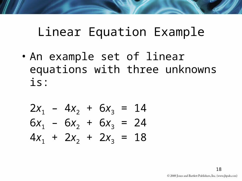
Linear Equation Example

• An example set of linear equations with three unknowns is:

2x1 – 4x2 + 6x3 = 146x1 – 6x2 + 6x3 = 244x1 + 2x2 + 2x3 = 18

19

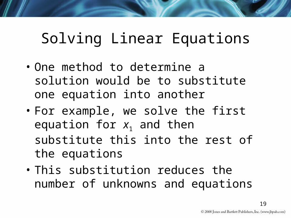
Solving Linear Equations

• One method to determine a solution would be to substitute one equation into another

• For example, we solve the first equation for x1 and then substitute this into the rest of the equations

• This substitution reduces the number of unknowns and equations

20

Solving Linear Equations

• If we repeat this, we get to one unknown and one equation and can then back up to get the values of the rest

• If there are many equations, this process can be time consuming, prone to error, and is not easily computerized

21

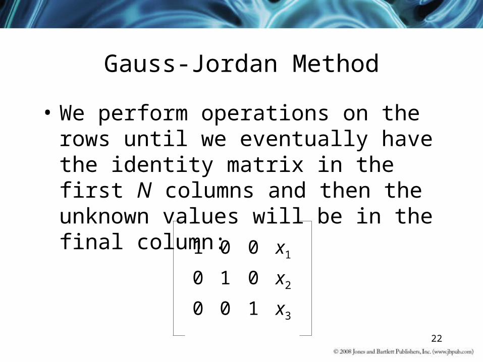
Gauss-Jordan Method

• This method is based on the previous idea

• We store the equation constants in a matrix with N rows and N+1 columns

• For the example, we would get:

2 -4 6 14

6 -6 6 24

4 2 2 18

22

Gauss-Jordan Method

• We perform operations on the rows until we eventually have the identity matrix in the first N columns and then the unknown values will be in the final column:

1 0 0 x1

0 1 0 x2

0 0 1 x3

23

Gauss-Jordan Method

• On each pass, we pick a new row and divide it by the first element that is not zero

• We then subtract multiples of this row from all of the others to create all zeros in a column except in this row

• When we have done this N times, each row will have one value of 1 and the last column will have the unknown values

24

Example

• Consider the example again:

• We begin by dividing the first row by 2, and then subtract 6 times it from the second row and 4 times it from the third row

2 -4 6 14

6 -6 6 24

4 2 2 18

25

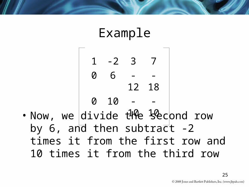
Example

• Now, we divide the second row by 6, and then subtract -2 times it from the first row and 10 times it from the third row

1 -2 3 7

0 6 -12 -18

0 10 -10 -10

26

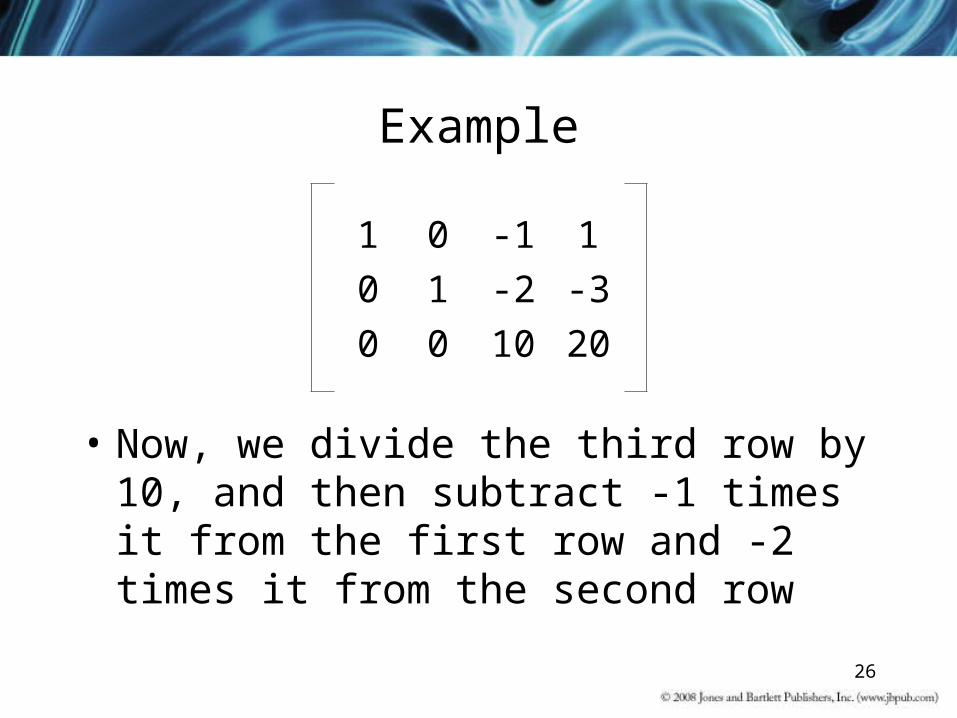
Example

• Now, we divide the third row by 10, and then subtract -1 times it from the first row and -2 times it from the second row

1 0 -1 1

0 1 -2 -3

0 0 10 20

27

Example

• This gives the result of:

• And we have that x1 = 3, x2 = 1, and x3 = 2

1 0 0 3

0 1 0 1

0 0 1 2