Embed Size (px)
Citation preview
1
Book: Constraint ProcessingAuthor: Rina Dechter
Chapter 10: Hybrids of Search and Inference Time-Space Tradeoffs
Zheying Jane Yang
Instructor: Dr. Berthe Choueiry
2
Outline
Combining Search and Inference--Hybrid Idea- Cycle Cutset Scheme
Hybrids: Conditioning-first- Hybrid Algorithm for Propositional Theories
Hybrids: Inference-first- The Super Cluster Tree Elimination - Decomposition into non-separable Components- Hybrids of hybrids
A case study of Combinational Circuits- Parameters of Primary Join Trees- Parameters Controlling Hybrids
Summary

3
Part IHybrids of Search and
Inference
4
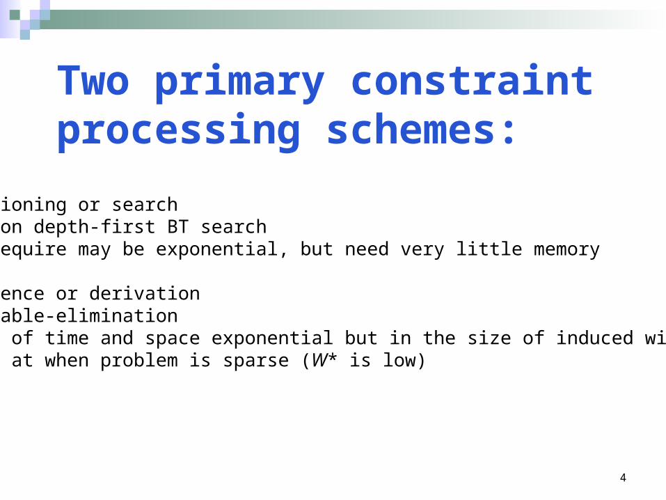
Two primary constraint processing schemes:
1. Conditioning or search Based on depth-first BT search time require may be exponential, but need very little memory
2. Inference or derivation Variable-elimination Both of time and space exponential but in the size of induced width. Good at when problem is sparse (W* is low)
5
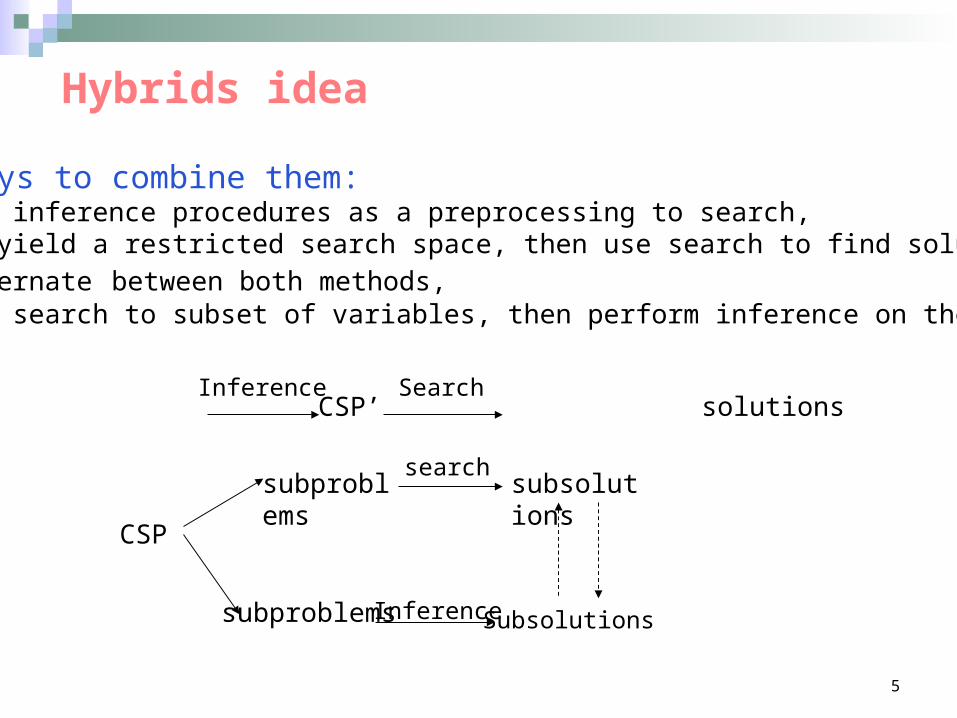
Hybrids idea
Two ways to combine them:• To use inference procedures as a preprocessing to search, then yield a restricted search space, then use search to find solutions.• To alternate between both methods, apply search to subset of variables, then perform inference on the rest
CSP CSP’ solutionsInference Search
CSP
subproblems
subproblems
search
Inference
subsolutions
Subsolutions
6
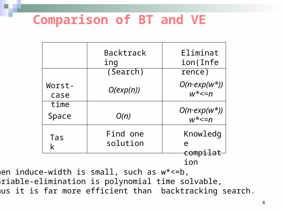
Backtracking(Search)
Elimination(Inference)
Worst-casetime
O(exp(n))O(n·exp(w*))
w*<=n
Space O(n)O(n·exp(w*))
w*<=n
Task Find one solution
Knowledge compilation
When induce-width is small, such as w*<=b, variable-elimination is polynomial time solvable, thus it is far more efficient than backtracking search.
Comparison of BT and VE
7
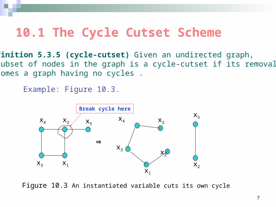
10.1 The Cycle Cutset Scheme
Definition 5.3.5 (cycle-cutset) Given an undirected graph, a subset of nodes in the graph is a cycle-cutset if its removalbecomes a graph having no cycles .
Example: Figure 10.3.
x5x2x4
x3 x1
x2
x4
x1
x3
x2
x5
x2
Break cycle here
Figure 10.3 An instantiated variable cuts its own cycle
8
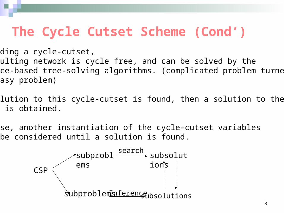
•When finding a cycle-cutset, The resulting network is cycle free, and can be solved by the inference-based tree-solving algorithms. (complicated problem turned to be easy problem)
• If a solution to this cycle-cutset is found, then a solution to the entire problem is obtained.
• Otherwise, another instantiation of the cycle-cutset variables should be considered until a solution is found.
The Cycle Cutset Scheme (Cond’)
CSP
subproblems
subproblems
search
Inference
subsolutions
subsolutions
9
Tradeoff between Finding a Small Cycle-cutsetand Using Search + Tree-Solving
A small cycle-cutset is desirable. However, finding a minimal-size cycle-cutset is NP-hard
Compromise between BT search and tree-solving algorithm
Step1: using BT to keep track of the connectivity status of the constraint graphStep2: As soon as the set of instantiated variables constitutes a cycle-cutset, the search algorithm is switched to the tree-solving algorithm.Step3: Either finding a consistent extension for the remaining variables find solution.Step4: Or no such extension exists, in this case, BT takes place again and try another instantiation.
10
B
A
CD
E
A
B E C D
C D C D
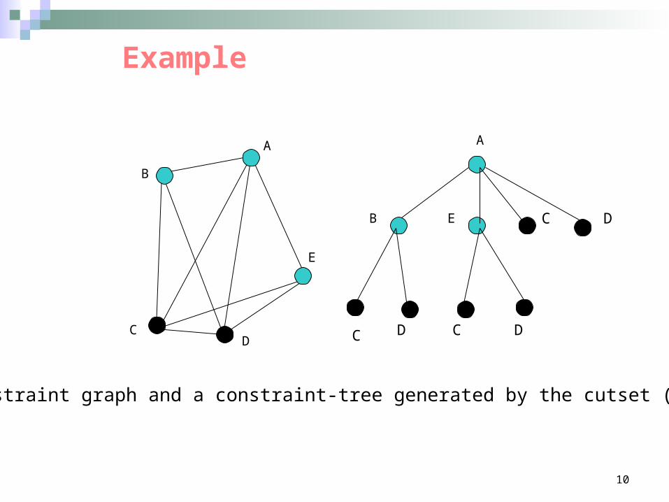
A constraint graph and a constraint-tree generated by the cutset (C,D)
Example
11
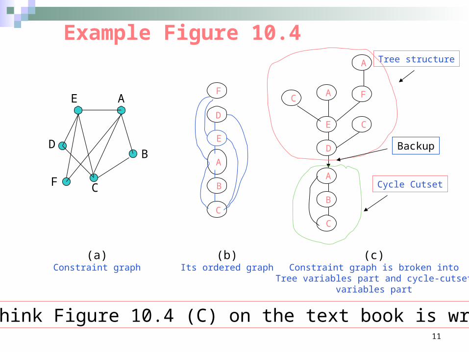
Example Figure 10.4
* I think Figure 10.4 (C) on the text book is wrong!
F
D
E
A
B
C
(a)Constraint graph
(b)Its ordered graph
A
AC
CE
F
D
C
B
Tree structure
Cycle Cutset
(c)Constraint graph is broken into
Tree variables part and cycle-cutsetvariables part
AE
D
F C
B
A
Backup
12
• When the original problem has a tree-constraint graph, the cycle-cutset scheme coincides with a tree-algorithm.
• When the constraint graph is complete, the algorithms reverts to regular backtracking. (Why?)
Two extreme cases:
13
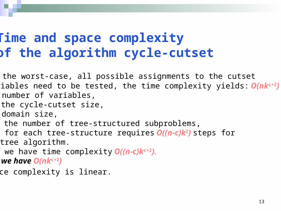
Time and space complexity of the algorithm cycle-cutset
• In the worst-case, all possible assignments to the cutset variables need to be tested, the time complexity yields: O(nkc+2) n is number of variables, c is the cycle-cutset size, k is domain size, kc is the number of tree-structured subproblems, then for each tree-structure requires O((n-c)k2) steps for the tree algorithm. Thus we have time complexity O((n-c)kc+2). Then we have O(nkc+2)• Space complexity is linear.
14
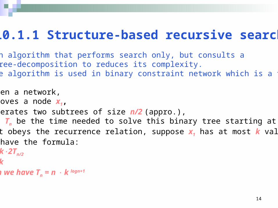
10.1.1 Structure-based recursive search
• An algorithm that performs search only, but consults a tree-decomposition to reduces its complexity.• The algorithm is used in binary constraint network which is a tree.
Given a network,Removes a node x1,Generates two subtrees of size n/2 (appro.),Let Tn be the time needed to solve this binary tree starting at x1, it obeys the recurrence relation, suppose x1 has at most k values,we have the formula: Tn = k2Tn/2 T1 = k Then we have Tn = n k logn+1
15
Theorem 10.1.3
A constraint problem with n variables and k values having a tree decomposition of tree-width w*, can be solved by recursive search in linear space and in O(nk2w*(logn+1) time
16
10.2 Hybrids: conditioning first
• Conditioning in cycle-cutset.
• This suggestion a framework of hybrid algorithms parameterized by a bound b on the induced-width of subproblems solved by inference.
• And conditioning in b-cutset.
17
Conditioning Set or b-cutset
The algorithm removes a set of cutset variables, gets a constraint graph with an induced-width bounded by b. we call such a conditioning set or b-cutset.
Definition 10.2.1 (b-cutset) Given a graph G, a subset of nodes is called a b-cutset iff when the subset is removed the resulting graph has an induced-width less than or equal to b. A minimal b-cutset of a graph has a smallest size among all b-cutsets of the graph. A cycle-cutset is a 1-cutset of a graph.
18
How to Find a b-cutset
Step1: Given a ordering d = {x1,…,xn} of G, a b-cutset relative to d is obtained by processing the nodes from last to first.Step2: When node x is processed, if its induced-width is greater than b, it is added to the b-cutset.
Step3: Else, its earlier neighbors are connected.Step4: The adjusted induced-width relative to a b-sutset is b.
Step5: A minimal b-cutset is a smallest among all b-cutset.
Definition 10.2.3 (finding a b-cutset) Given a graph G = (V,E) and a constant b, find a minimal b-cutset. Namely, find a smallest subset of nodes U, such that G’ = (V-U, E’), where E’ includes all the edges in E that are not incident to nodes in U, has induced-width less than or equal b.
19
The Purpose of Algorithm elim-cond(b)
• Original problem is divided two smaller parts: Cutset variables Remaining variables (subproblems)
• We can runs BT search on the cutset variables• Run bucket elimination on the remaining variables.
This yields elim-cond(b) algorithm The constant b can be used to control the balance between search and variable-elimination, and thus effect the tradeoff between time and space.
20
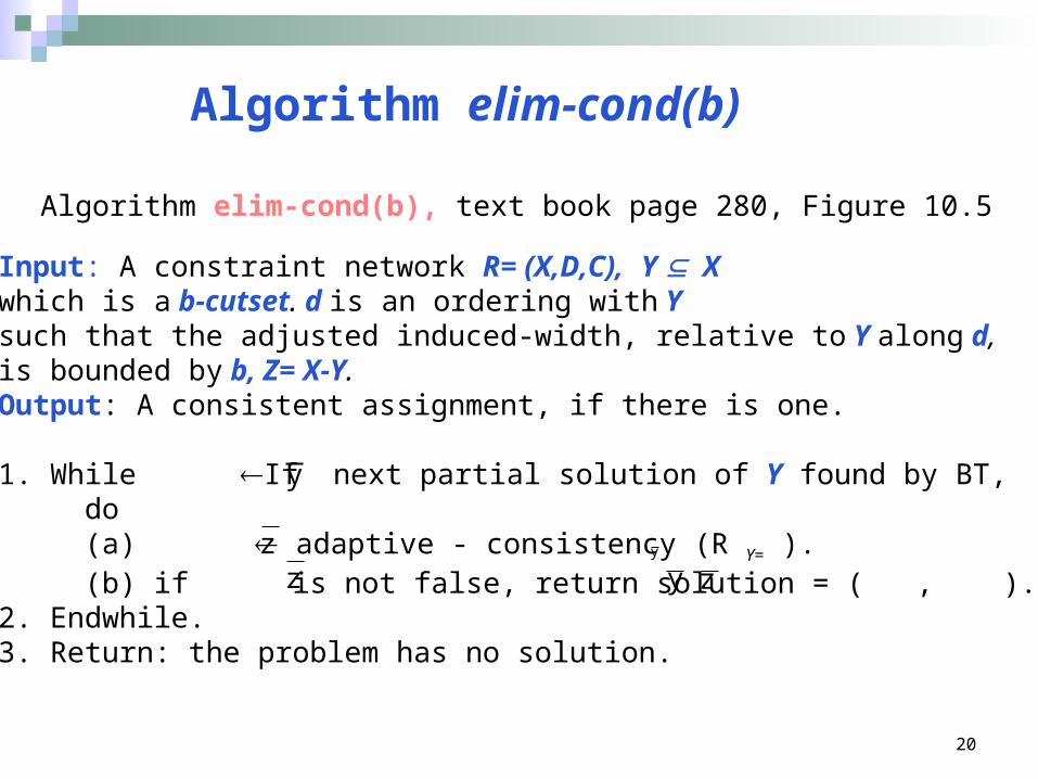
Algorithm elim-cond(b)
Algorithm elim-cond(b), text book page 280, Figure 10.5
Input: A constraint network R= (X,D,C), Y Xwhich is a b-cutset. d is an ordering with Y such that the adjusted induced-width, relative to Y along d, is bounded by b, Z= X-Y. Output: A consistent assignment, if there is one.
1. While If next partial solution of Y found by BT, do (a) adaptive - consistency (R Y= ). (b) if is not false, return solution = ( , ).2. Endwhile.3. Return: the problem has no solution.
y
z y
z zy
21
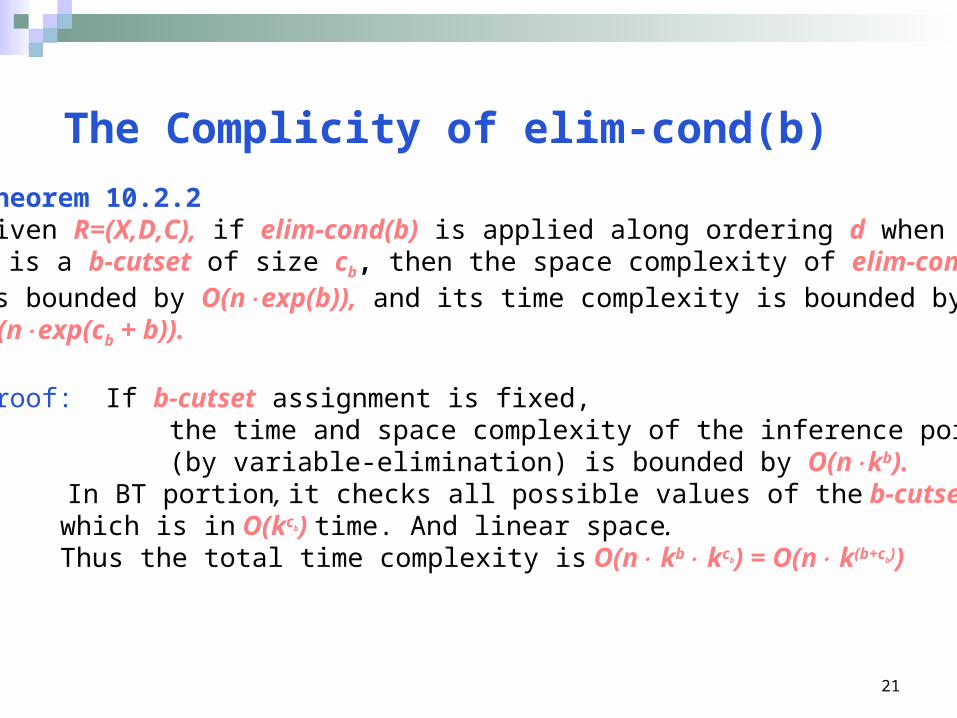
The Complicity of elim-cond(b)
Theorem 10.2.2Given R=(X,D,C), if elim-cond(b) is applied along ordering d when Y is a b-cutset of size cb, then the space complexity of elim-cond(b) is bounded by O(nexp(b)), and its time complexity is bounded by O(nexp(cb + b)).
Proof: If b-cutset assignment is fixed, the time and space complexity of the inference portion (by variable-elimination) is bounded by O(nkb). In BT portion, it checks all possible values of the b-cutset, which is in O(kcb) time. And linear space. Thus the total time complexity is O(n kb kcb) = O(n k(b+cb))

22
Part IITrade-off between
search and inference
23
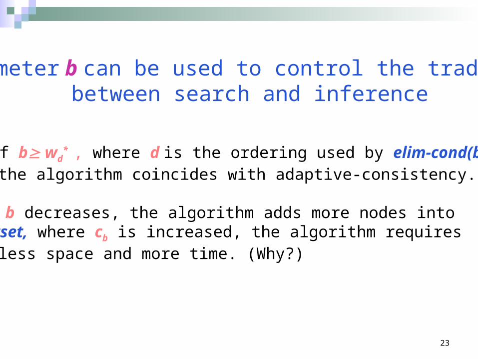
If b wd* , where d is the ordering used by elim-cond(b)
the algorithm coincides with adaptive-consistency. As b decreases, the algorithm adds more nodes into cutset, where cb is increased, the algorithm requires less space and more time. (Why?)
Parameter b can be used to control the trade-off between search and inference
24
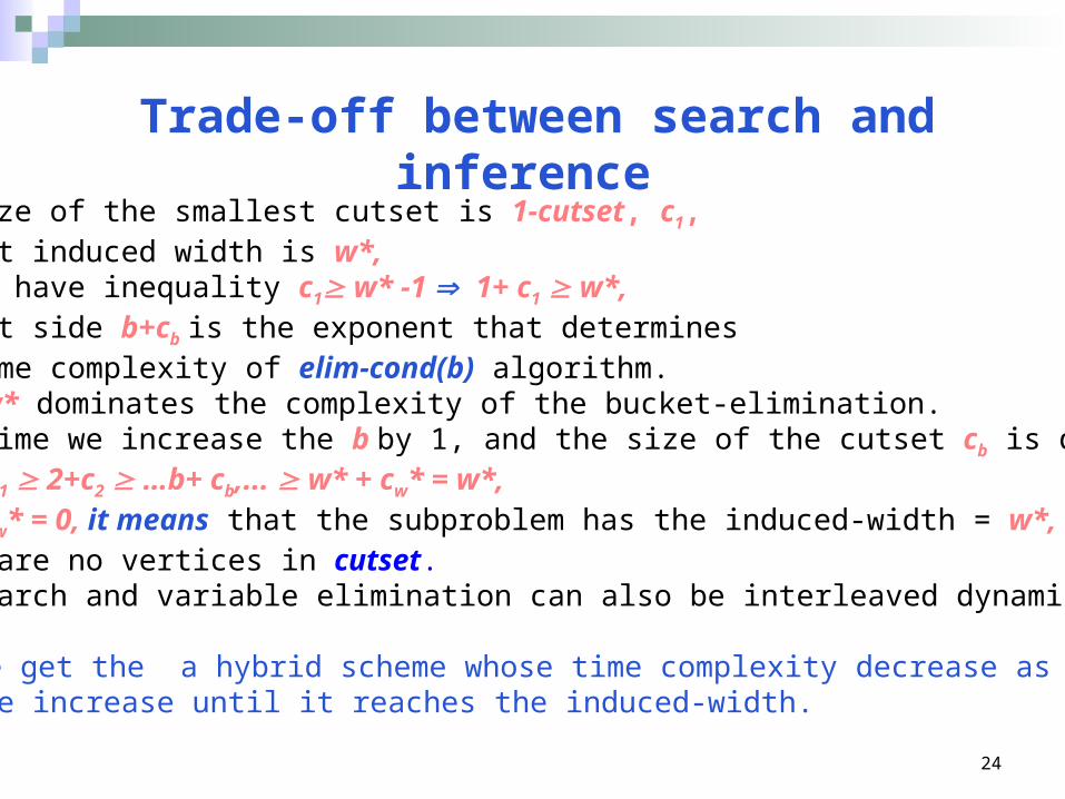
• Let size of the smallest cutset is 1-cutset, c1,• Smallest induced width is w*, • Then we have inequality c1 w* -1 1+ c1 w*,• The left side b+cb is the exponent that determines the time complexity of elim-cond(b) algorithm.• While w* dominates the complexity of the bucket-elimination. • Each time we increase the b by 1, and the size of the cutset cb is decreased.
1+ c1 2+c2 …b+ cb,... w* + cw* = w*, When cw* = 0, it means that the subproblem has the induced-width = w*, there are no vertices in cutset. • Thus search and variable elimination can also be interleaved dynamically.
Thus we get the a hybrid scheme whose time complexity decrease as its space increase until it reaches the induced-width.
Trade-off between search and inference
25
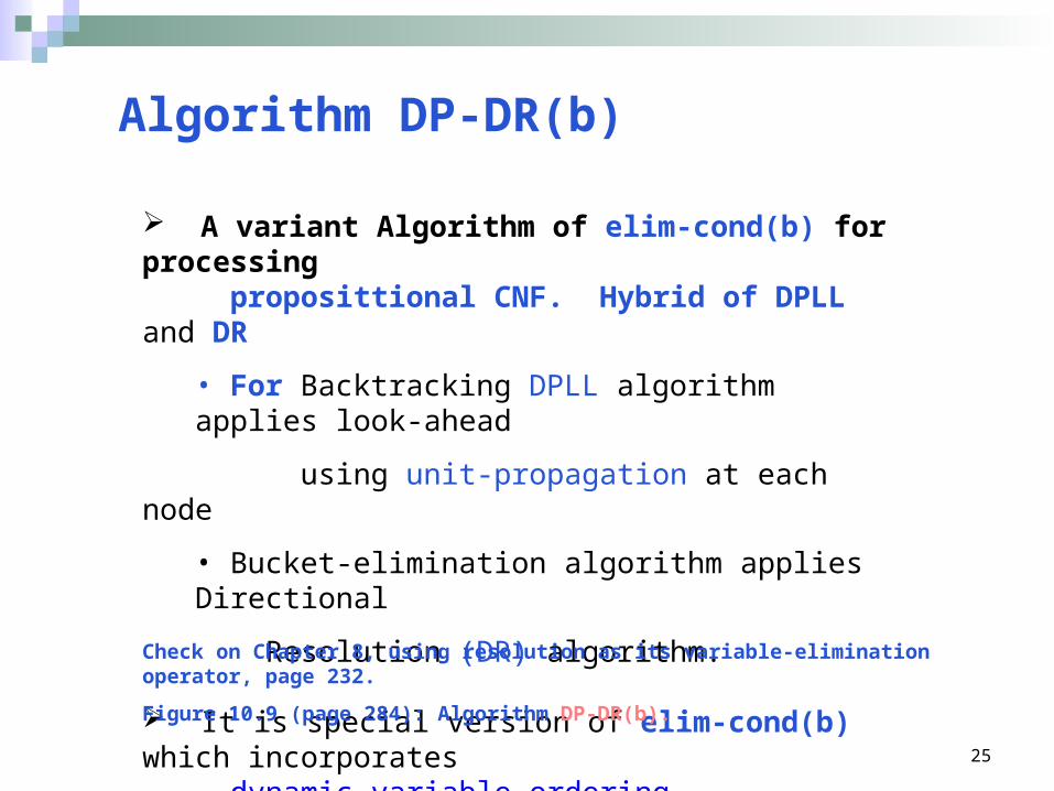
Algorithm DP-DR(b)
A variant Algorithm of elim-cond(b) for processing proposittional CNF. Hybrid of DPLL and DR
• For Backtracking DPLL algorithm applies look-ahead
using unit-propagation at each node
• Bucket-elimination algorithm applies Directional
Resolution (DR) algorithm.
It is special version of elim-cond(b) which incorporates dynamic variable-ordering.
Check on Chapter 8, using resolution as its variable-elimination operator, page 232.
Figure 10.9 (page 284): Algorithm DP-DR(b).
26
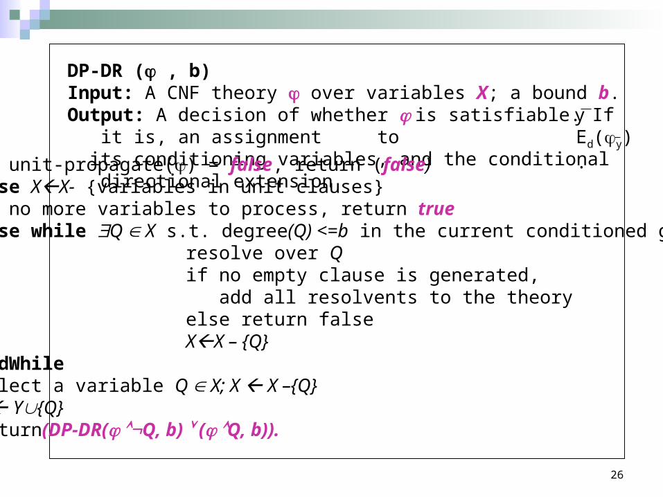
DP-DR ( , b)Input: A CNF theory over variables X; a bound b.Output: A decision of whether is satisfiable. If it is, an assignment to its conditioning variables, and the conditional directional extension
y Ed(y).
•If unit-propagate() = false, return (false)•Else XX- {variables in unit clauses}•If no more variables to process, return true•Else while Q X s.t. degree(Q) <=b in the current conditioned graph• resolve over Q• if no empty clause is generated,• add all resolvents to the theory• else return false• XX – {Q}•EndWhile•Select a variable Q X; X X –{Q}•Y Y{Q}•Return(DP-DR( Q, b) ( Q, b)).
27
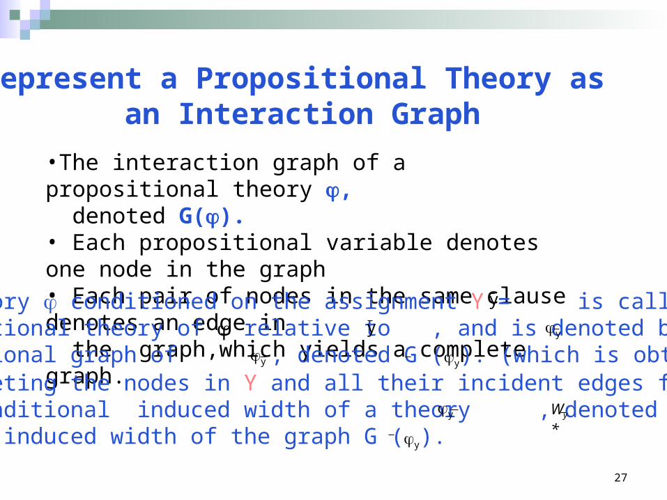
Represent a Propositional Theory as an Interaction Graph
•The interaction graph of a propositional theory , denoted G(). • Each propositional variable denotes one node in the graph• Each pair of nodes in the same clause denotes an edge in the graph,which yields a complete graph.
•The theory conditioned on the assignment Y = is called a conditional theory of relative to , and is denoted by . • Conditional graph of , denoted G (y). (which is obtained by deleting the nodes in Y and all their incident edges from G().• The conditional induced width of a theory , denoted , is the induced width of the graph G (y).
y
y y
y Wy*
y
28
A
B C
E
DA
B C
E
DResolution over A
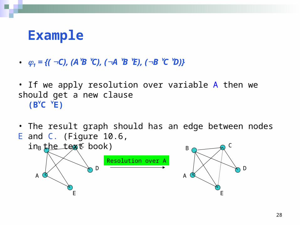
• 1 = {( C), (AB C), (A B E), (B C D)}
• If we apply resolution over variable A then we should get a new clause (BC E)
• The result graph should has an edge between nodes E and C. (Figure 10.6, in the text book)
Example
29
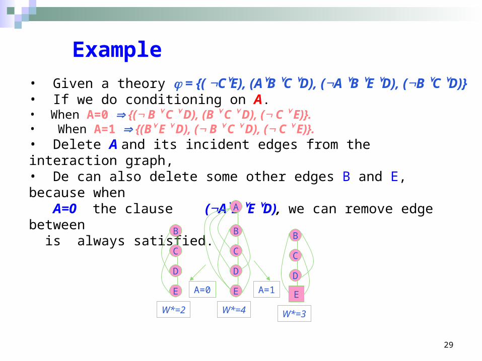
• Given a theory = {( CE), (AB C D), (A B E D), (B C D)} • If we do conditioning on A.• When A=0 {( B C D), (B C D), ( C E)}. • When A=1 {(B E D), ( B C D), ( C E)}.• Delete A and its incident edges from the interaction graph, • De can also delete some other edges B and E, because when A=0 the clause (AB E D), we can remove edge between is always satisfied.
B
C
D
E A=1A=0
B
C
D
E
A
W*=4W*=2
B
C
D
W*=3
E
Example
30
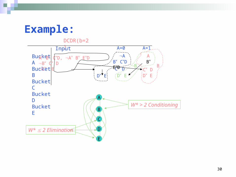
Example:DCDR(b=2)
Bucket ABucket BBucket CBucket DBucket E
Input
A B CD, A B EDB C DC E C D
A=0
A
A=1
AB CD B ED
B BC DD ED ED E
B
C
D
E
A
W* > 2 Conditioning
W* 2 Elimination
31
Complexity of DP-DR(b)
Theorem 10.2.5 • The time complexity of algorithm DP-DR(b) is O(nexp(cb + b)), where cb is the largest cutset to be conditioned upon.
• The space complexity is O(nexp(b)).
32
Empirical evaluation of DP-DR (b)
Evaluation of DP-DR(b) on Conditioning-first hybrids Empirial results from experiments with different structured CNFs.
• Use random uniform 3-CNFs with 100 variables and 400 clauses• (2, 5) -trees with 40 cliques and 15 clauses per clique• (4, 8) -trees with 50 cliques and 20 clauses per clique• In general, (k, m) -trees are trees of cliques each having m+k nodes
and separators size of k. • The randomly generated 3-CNFs were designed to have an interaction
graph that corresponds to (k, m)-trees. The performance of DP-DR(b) depends on the induced width of the theories. When b=5, the overall performance is best. See Figure 10.10, on page 285.
33
Part III
Non-separable components and
tree-decomposition
34
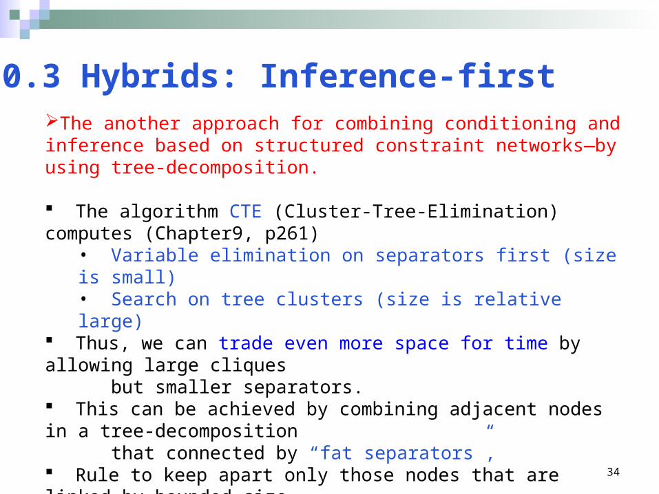
10.3 Hybrids: Inference-firstThe another approach for combining conditioning and inference based on structured constraint networks—by using tree-decomposition. The algorithm CTE (Cluster-Tree-Elimination) computes (Chapter9, p261)
• Variable elimination on separators first (size is small) • Search on tree clusters (size is relative large)
Thus, we can trade even more space for time by allowing large cliques but smaller separators. This can be achieved by combining adjacent nodes in a tree-decomposition that connected by “fat separators”, Rule to keep apart only those nodes that are linked by bounded size separators.
35
Tree Decomposition
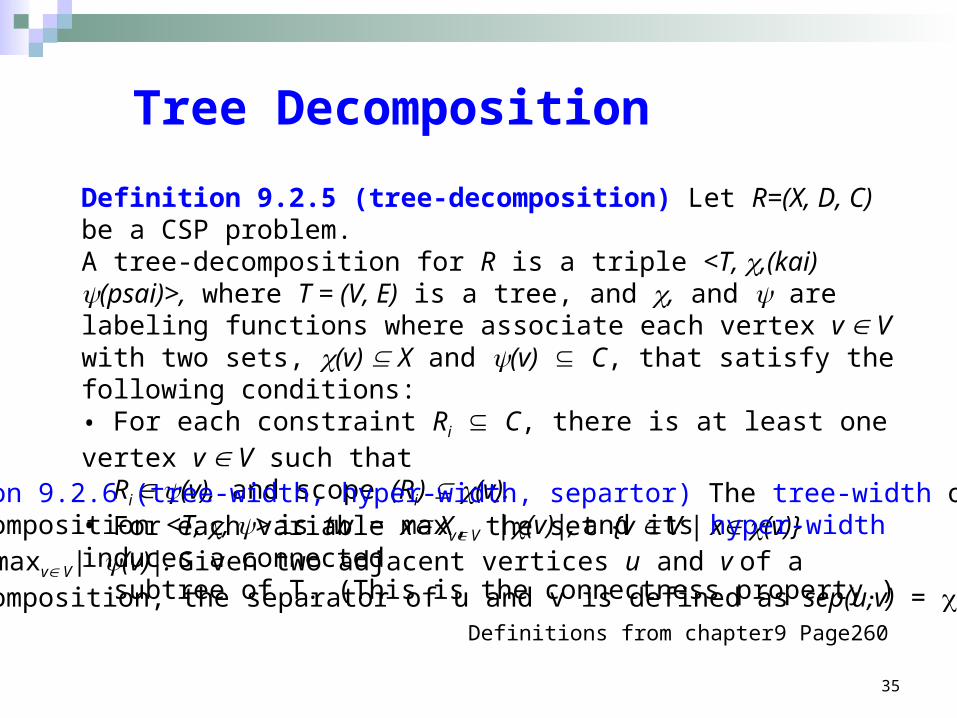
Definition 9.2.5 (tree-decomposition) Let R=(X, D, C) be a CSP problem.A tree-decomposition for R is a triple <T, ,(kai) (psai)>, where T = (V, E) is a tree, and , and are labeling functions where associate each vertex v V with two sets, (v) X and (v) C, that satisfy the following conditions:• For each constraint Ri C, there is at least one vertex v V such that Ri (v), and scope (Ri) (v).• For each variable x X, the set {v V | x (v)} induces a connected subtree of T. (This is the connectness property.)
Definition 9.2.6 (tree-width, hyper-width, separtor) The tree-width of atree-decomposition <T, , > is tw = maxv V |(v)|, and its hyper-widthis hw = maxv V| (v)|. Given two adjacent vertices u and v of a tree-decomposition, the separator of u and v is defined as sep(u,v) = (u) (v).
Definitions from chapter9 Page260
36
Assume a CSP problem has a tree-decomposition, which has tree- width r and separator size s.
Assume the space restrictions do not allow memory space up to O(exp(s)) One way to overcome this problem is to collapse these nodes in the tree that are connected by large separators
let previous connected two nodes include the variables and constraints The resulting tree-decomposition will has larger subproblems but smaller separators. As s decrease, both r and hw increase.
Tree-Decomposition
37
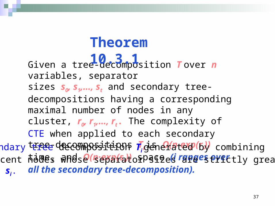
Given a tree-decomposition T over n variables, separator sizes s0, s1,…, st and secondary tree-decompositions having a corresponding maximal number of nodes in any cluster, r0, r1,…, rt. The complexity of CTE when applied to each secondary tree-decompositions Ti is O(n·exp(ri)) time, and O(n·exp(si)) space (i ranges over all the secondary tree-decomposition).
• Secondary tree decomposition Ti generated by combining adjacent nodes whose separator sizes are strictly greater than si.
Theorem 10.3.1
38
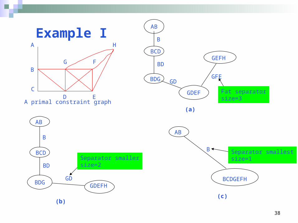
Example IA
B
C
G
D
F
E
H
AB
GDEF
BCD
BDG
GEFH
B
BD
GDGFE
Fat separatorsize=3
BDG
AB
BCD
GDEFH
B
BD
GD
Separator smallersize=2
AB
BCDGEFH
B Separator smallestsize=1
(a)
(b)(c)
A primal constraint graph
39
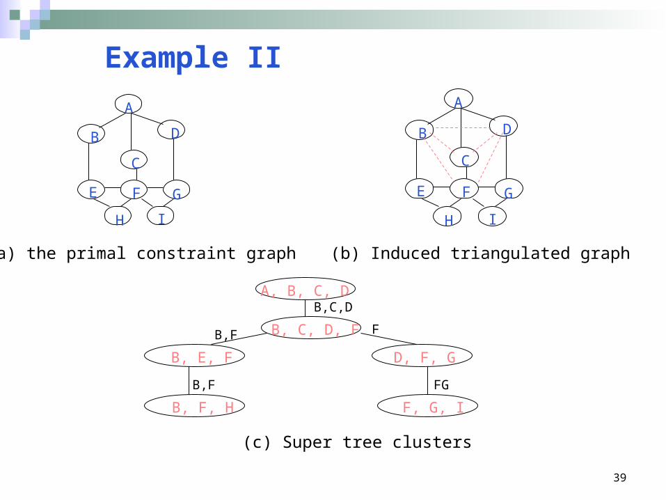
Example II
A
B
C
D
E F G
H I
(a) the primal constraint graph (b) Induced triangulated graph
A
B
C
D
E F G
H I
A, B, C, D
B, C, D, F
B, E, F D, F, G
F, G, I B, F, H
(c) Super tree clusters
B,C,D
B,F F
B,F FG
40
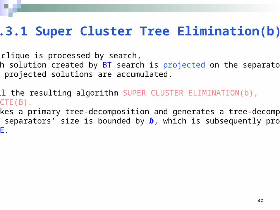
Each clique is processed by search, • each solution created by BT search is projected on the separator • the projected solutions are accumulated.
We call the resulting algorithm SUPER CLUSTER ELIMINATION(b), or SCTE(B).• It takes a primary tree-decomposition and generates a tree-decomposition whose separators’ size is bounded by b, which is subsequently processed by CTE.
10.3.1 Super Cluster Tree Elimination(b)
41
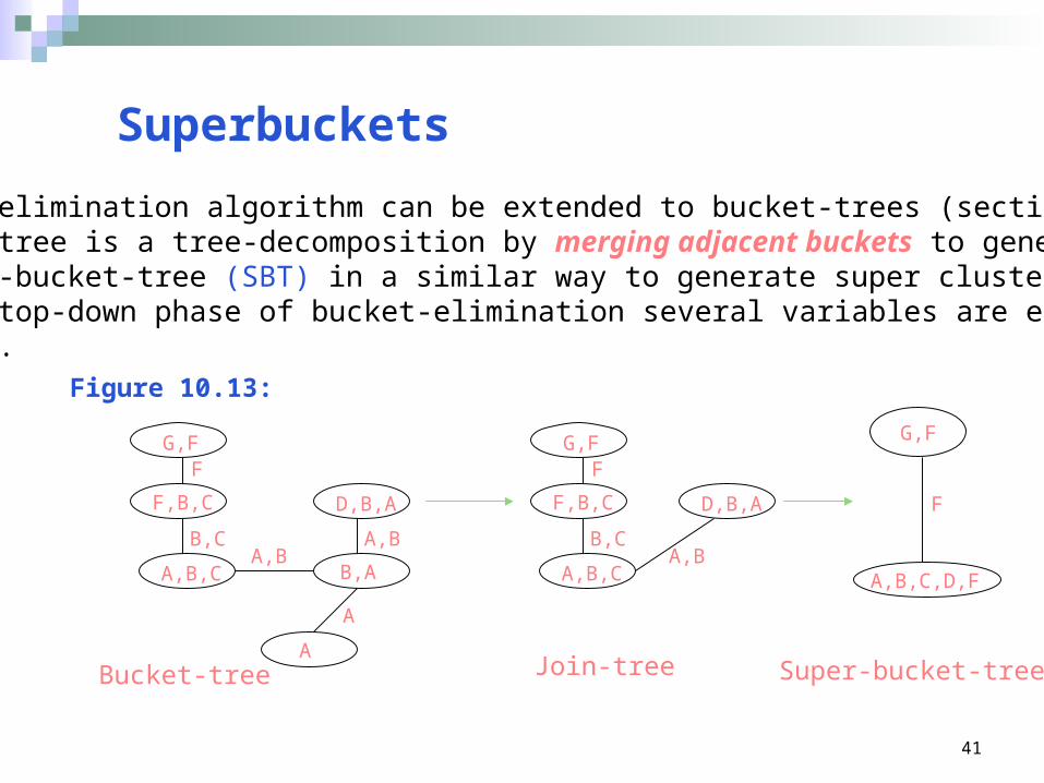
Superbuckets
Bucket-elimination algorithm can be extended to bucket-trees (section 9.3)Bucket-tree is a tree-decomposition by merging adjacent buckets to generatea super-bucket-tree (SBT) in a similar way to generate super clusters.In the top-down phase of bucket-elimination several variables are eliminatedat once.
Figure 10.13:
G,F
F,B,C
A,B,C
F
B,C
G,F
F,B,C
A,B,C
F
B,CA,B
B,A
A
D,B,A
A,B
A
A,B
G,F
D,B,A
A,B,C,D,F
F
Bucket-tree Join-tree Super-bucket-tree
42
A connected graph G = (V, E) is said to have separation node v if there exist nodes a and b such that all paths connection a and b pass through v.
• A graph that has a separation node is called separable, and one that has none is called non-separable. • A subgraph with no separation nodes is called a non-separable component (or a bi-connected component).
Definition 10.3.3 (non-separable components)
43
10.3.2 Decomposition into non-separable components
Generally we cannot find the best-decomposition having a bounded separators’ size in polynomial time.Tree-decomposition--all the separators are singeton variables: It requires only linear space {O(n·exp(sep)), where size of sep=1).
• The variables of the nodes are those appearing in each component
• The constraints can be placed into a component that contains
their scopes
• Applying CTE to such a tree requires linear space, (CTE space
complexity is O(N·exp(sep)), chapter9, page263)
• Each node corresponds to a component
• But it is time exponential in the components’ sizes
44
G C3 C4
A
B
D
C
F
E
H
I
J
(a)
F E
C2
C
C1
(b)
C,F,E
G,F,J
E,H,I
A,B,C,D
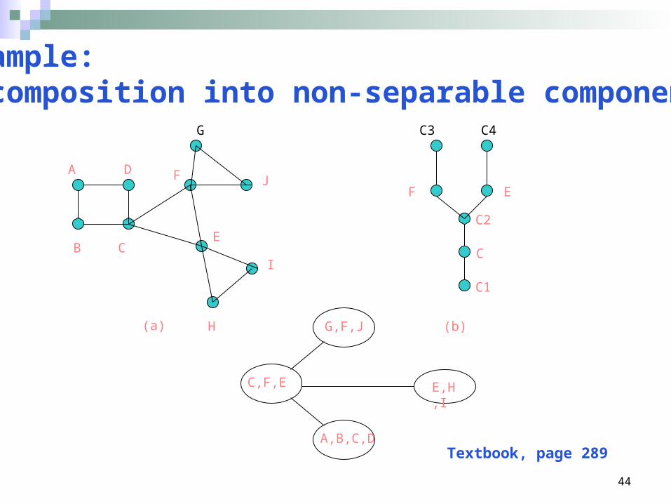
Example: Decomposition into non-separable components
Textbook, page 289
45
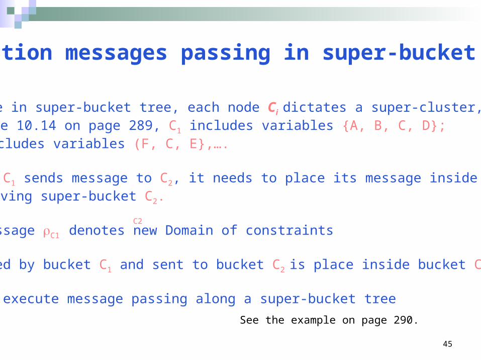
Execution messages passing in super-bucket tree
Because in super-bucket tree, each node Ci dictates a super-cluster, i.e., Figure 10.14 on page 289, C1 includes variables {A, B, C, D}; C2 includes variables (F, C, E},….
If the C1 sends message to C2, it needs to place its message inside the receiving super-bucket C2.
The message C1 denotes new Domain of constraints
Computed by bucket C1 and sent to bucket C2 is place inside bucket C2.
How to execute message passing along a super-bucket tree
C2
See the example on page 290.
46
Part IVHybrids of hybrids
47
10.3.3 Hybrids of hybrids
Advantage: The space complexity of this algorithm is linear but its time complexity can be much better than the cycle-cutset scheme or the non-separable component alone.
Example: Case study for c432, c499,… see Figure 10.19
48
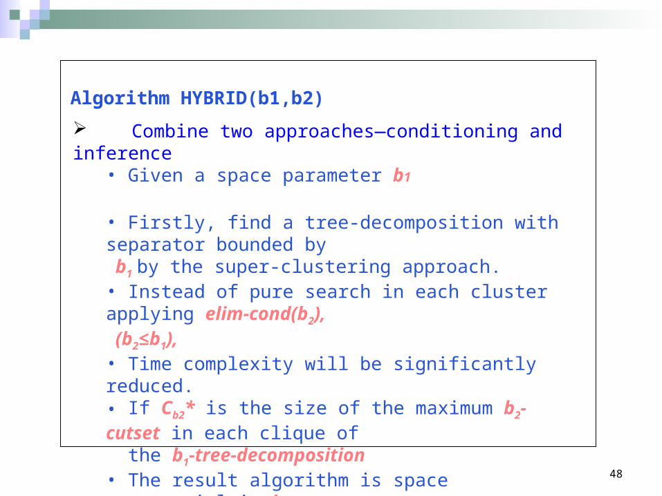
Combine two approaches—conditioning and inference• Given a space parameter b1
• Firstly, find a tree-decomposition with separator bounded by b1 by the super-clustering approach.• Instead of pure search in each cluster applying elim-cond(b2), (b2≤b1),• Time complexity will be significantly reduced. • If Cb2* is the size of the maximum b2-cutset in each clique of the b1-tree-decomposition• The result algorithm is space exponential in b1
(separator is restricted by b1)• But time exponential in Cb2* (cycle-cutsize is bound by b2)
Algorithm HYBRID(b1,b2)
49
Two special cases
1. Apply the cycle-cutset scheme (hybrid(b1,1)) in each clique. Real circuits problem—for circuit diagnosis tasks shows that the reduction in complexity bounds for complex circuits is tremendous.
2. When b1=b2, for b=1, hybrid(1,1) corresponds to applying the non-separable components as a tree-decomposition and utilizing the cycle-cutset in each component.
50
Method Using triangulation approach to decompose each circuit graph.
• Selecting an ordering for the nodes• Triangulating the graph • Generating the induced graph • Identifying its maximum cliques (maximal-cardinality)
o Using heuristic the min-degree ordering, will yield the smallest cliques sizes and separators.
See Fig 10.18
10.4 A case study of combinatorial circuitsTextbook Page 291-294
51
Parameters of primary join trees
For each primary join tree generated, three parameters are computed:
(1) The size of cliques,(2) The size of cycle-cutsets in each of the subgraphs defined by
clique sizes.(3) The size of the separator sets.
• The nodes of the join tree are labeled by the clique (cluster) sizes• In Figure 10.18 shows us, some cliques and separators require memory space exponential in 28 for circuit c432 and exponential in 89 for circuit C3540.• This is unacceptable using hybrid(b,1).• We can select parameter b to control the balance of time and space.• Figure 10.19
52
Parameters controlling hybrids
• For each separator size, si, in primary join tree T0 listed from largest to smallest, • A tree decomposition Ti generated by combining adjacent clusters whose separators’ sizes are strictly larger than si.• Ci denotes the largest cycle-cutset size computed in any cluster of Ti. • Secondary join tree are indexed by the separator sizes of the primary tree, which range from 1 to 23 ( see Figure 10.20).
• As the separator size decreases, the maximum clique size increases, the both of the size and depth of the tree decreases.• The clique size for the root node is much larger than for all other nodes, and it increases as the size of the separators decreases.
53
Summary This chapter presents a structured based hybrid scheme that uses inference and search as its two extremes Using single design parameter b, to allow the users to control the storage-time tradeoff in accordance with the problem domain and the available resources. Two architectures for hybrids are proposed:
The conditioning first• Find a small variable set Y, assign them values, the result
subproblems have low induced width, and solve them by variable-elimination.
The inference first• Limit space by using tree-decompositions whose separator size is
bounded by b. And further a hybrid of the two hybrids allows even better time complexity for every fixed space restrictions
54
Reference
1. R. Dechter, Constraint Processing. 2. Jeff Bilmes, Introduction to Graphical Models. Spring 2002, scribs3. R. Dechter. Enhancement schemes for constraint processing: Backjumping, learning and cutset decomposition. AI, 41:273-312, 19904. R. Dechter and J. Pearl. The cycle-cutset method for improving search
performance in AI applications. In Processing of the 3rd IEEE Conference on AI Application, pages 224-230, Orlando, Florida, 1987.5. R. Dechter and J. Peral. Tree clustering for constraint networks. AI, pages 353-366, 1989.