Embed Size (px)
Citation preview
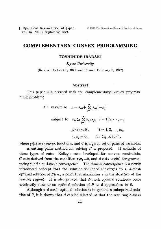
J. Operations Research Soc. of Japan Vol. 15, No. 3, September 1972.
COMPLEMENTARY CONVEX PROGRAMMING
TOSHIHIDE IBARAKI
Kyoto University
(Received October 8, 1971 and Revised February 9, 1972)
Abstract
This paper is concerned with the complementary convex program
ming problem:
.. P: maximize z = aoo+ ;E aoj (-Xj) ,-1
subject to ..
a.o~ ;E a'j Xj, i = 1,2, . .. , m1 ,-1 i= 1,2,· .. ,m2
XpX, = 0, for (xp, Xq) E C ,
where g.(x) are convex functions, and C is a given set of pairs of variables. A cutting plane method for solving P is proposed. It consists of
three types of cuts: Kelley's cuts developed for convex constraints,
C-cuts derived from the condition xpX'l =0, and J-cuts useful for guaran
teeing the finite J-mesh convergence. The J-mesh convergence is a newly introduced concept that the solution sequence converges to a J-mesh
optimal solution of P(i.e., a point that maximizes z in the J-lattice of the feasible region). It is also proved that J-mesh optimal solutions come
arbitrarily close to an optimal solution of P as J approaches to O.
Although a J-mesh optimal solution is in general a suboptimal solu
tion of P, it is shown that J can be selected so that the resulting J-mesh
138
© 1972 The Operations Research Society of Japan
Complementarg Convex Programming 139
optimal solution is an exact optimal solution in case P has no convex
constraint (i.e., mz=O).
1. Introduction
In this paper, we will deal with complementary convex programming
problems (CCP problems), which are convex programming problems with
one more constraint, the complementarity condition (see (2) below),
added. Several application areas of the complementarity condition are
discussed in [6J, [7J. A cutting plane method for solving a CCP problem will be developed.
It is guaranteed to converge to a J-mesh optimal solution in a finite number of steps. The J-mesh optimal solution is a lattice point of the
J-mesh in the feasible region of the problem, which maximizes the ob
jective value. It is in practice a good approximate solution to an optimal
solution of the given problem. There are cases in which J-mesh optimal solution is also a real optimal solution. One is when an additional
constraint that makes only lattice points of J-mesh feasible (consider the
integer programming problem which assumes J = 1) is imposed. The other is a complementary linear programming problem (Le., LP problem
with the complementarity condition) for which it is known that J can
be selected so that the resulting J-mesh optimal solution is a real optimal solution.
The cutting plane method presented in this paper consists of three
types of cuts: Kelley's cut [9J for the convex constraints, C-cuts for the complementarity condition and J-cuts for guaranteeing the finite J-mesh convergence. J-cuts are developed by extending the concept of
Gomory's cuts [3J, [4J, [5J for integer constraints.
First let us define a convex programming (CVP) problem* by
n Q: maximize z(x) = aoo+ ;E aOj(-xj)
J-1
* Althollgh the second constraints Xj= - (-lfj) are not really restrictions, they must be here to carry Ollt the simplex method based on the lexicographical order, discussed in Section 3.
Copyright © by ORSJ. Unauthorized reproduction of this article is prohibited.
140 Toshihide Ibaraki
n (I ) subject to X .. +; = a;o + ~ a;j (-Xj)' i = 1,2, ... , ml
;-1
X;=-(-Xj), j=I,2, ... ,n
X,+; = -g; (x) , i = 1,2, ... , m 2
Xk20, k= 1,2, ···,n+ml+m2
where r=n +m1, X= (Xl' X 2, .. , x .. ) ER", a;j E R, and g;(x) are convex functions of X. x,,+;ER, i=l, 2, . . ,ml+m2 are slack variables. Note that the objective function is linear. Q has ml linear constraints (constraints given by linear inequalities) and m2 convex constraints.
Let C be a set of pairs of variables Xl> X2, •• , X,.
The complementarity condition is defined for C by
(2) xp Xq = 0 for every (xp, x,) E C .
A complementary convex programming (CCP) problem P is a CVP problem
Q restricted further by the complementarity condition (2). For problem 5(=P, Q or anything else), solutions (Xl' X2,' .,x,,)ER"
are feasible if they satisfy 5's constraints. The feasible region of 5, F(5),
is the set of all feasible solutions. An optimal solution x of 5 is a feasible solution satisfying z(x) 2 z(x) for all xEF(5). The set of all optimal solutions of 5 is denoted by 0(5).
2. ..::2-Mesh Optimality
The A-mesh R,/,cR" is defined by the set of all vectors xER" such that their components are all multiples of A, where .1>0 and AER. In other words, xERA" if and only if x=Ax' where x' is an integer vector. Let
FA (5) =F(5) n R,t,
where 5 is P, Q or anything else. xEFA(5) is a A-mesh optimal solution
of 5 if x satisfies z(X) 2 z(x) for all xEFA(5). We denote the set of all A-mesh optimal solutions by 0 A(5).
Copyright © by ORSJ. Unauthorized reproduction of this article is prohibited.
Complementarg Convex Programming 141
Throughout this paper, we assume that z and X .. +i, i=l, 2, .. ,ml'
also take on multiples of J only for all x E R,,/. This assumption is for example accomplished if
(3) aoo=O, aoj: integers, /= 1,2, "',n
aio E R4 , aij: integers, i = 1,2, .. " ml
1·=12 .. ·n • " J
hold in (1). (In practice this does not lose any generality because if original coefficients and J are all rational numbers, we can multiply a positive number with those coefficients so that (3) may hold true.)
The last half of the condition (3) may be deleted from the assump
tion if we regard each linear constraint
n x,,+i=aio+ I: aij I-Xj) , X .. +i:;::: 0
j-l
as a special case of the convex constraint
X'+i = - g; (x) , X,+; :;::: ()
(i.e., ml is set to 0 and m2 is set to 1nl +m2)' In this case, however, it should be noticed that variables xp and Xg of the complementarity condition cannot be variables X;'+i, i = 1, 2, .. , ml .
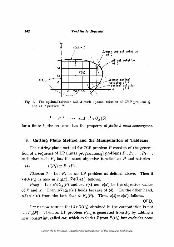
J-mesh optimal solutions of a CCP problem and a CVP problem are illustrated in Fig. 1. F(Q) of the given CVP problem Q is the region surrounded by Xl and X2 axes, and the curve given by g(x) =0. J-mesh optimal solution of Q is also indicated in Fig. 1. On the other hand, F(P) is given by two line segments on the Xl axis and X2 axis, because of the
complementarity condition XlX2=O. Thus the optimal solution and Jmesh optimal solution of P are on the Xl axis as shown in Fig. 1.
Consider a sequence of solutions
If .the sequence {Xk} converges to a .~-mesh optimal solution of S, it is said to have the property ofJ-mesh convergence. In particular, if
Copyright © by ORSJ. Unauthorized reproduction of this article is prohibited.
142
F(P)
Toshihide Ibaraki
g(x) = 0
A-mesh optimal sol ution of Q
optimal sol ution of Q
3A~-r--+--+--+-~~
A-mesh optimal solution of P ~ optimal solution
~~~~--~~T-~~'~,~--~x1 ofP , , \ \
Fig. 1. The optimal solution and A-mesh optimal solution of CVP problem Q and CCP problem P.
Xk = xk +1 = . .. and xk E O,d (5)
for a finite k, the sequence has the property of finite A-mesh convergence.
3. Cutting Plane Method and the Manipulation of Tableaus
The cutting plane method for CCP problem P consists of the generation of a sequence of LP (linear programming) problems PI' P 2, • • , P k , •• ,
such that each P k has the same objective function as P and satisfies
(4) F(Pk ) ~ F,d (P) .
Theorem 1: Let P k be an LP problem as defined above. Then if XEO(Pk ) is also in F"iP), XEO,d(P) follows.
Proof: Let x' E ° ,d(P) and let z(x) and z(x') be the objective values of x and x'. Then z(x) ~ z(x') holds because of (4). On the other hand, z(x) sz(x') from the fact that xEF ,d(P). Thus, z(X) =z(x') follows.
QED. Let us now assume that x E ° (Pk) obtained in the computation is not
in F ,d(P). Then, an LP problem P k+l is generated froro Plo by adding a new constraint, called cut, which excludes x froro F(Pk ) but excludes none
Copyright © by ORSJ. Unauthorized reproduction of this article is prohibited.
Complementary Convex Programming 143
of points in F ,d(P). Thus Pk+l also satisfies (4) with k replaced by k+ 1. This process is repeated until a J-mesh optimal solution of P is obtained.
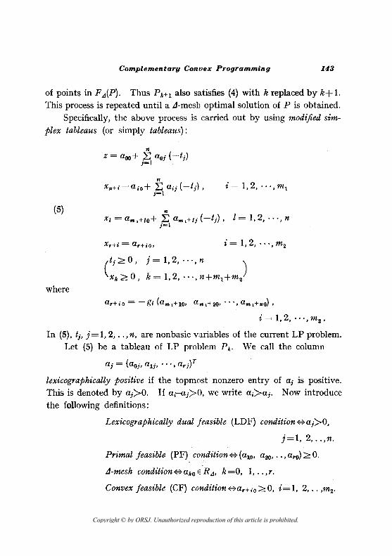
Specifically. the above process is carried out by using modified sim
plex tableaus (or simply tableaus):
(5)
where
i = 1.2 •...• m l
n XI = am,+IO+ L am,+/j (-tj ). I = 1.2 •...• n
j-l
X,+i = a,+io. i=I.2 •...• m2
Cj:?; 0. j = 1.2 •.. '. n )
Xk :?; 0. k = 1.2 •.. '. n+ml +m2
i = 1.2 •...• m2 •
In (5). tj. j = 1.2 •..• n. are nonbasic variables of the current LP problem. Let (5) be a tableau of LP problem P k • We call the column
lexicographically positive if the topmost nonzero entry of aj is positive. This is denoted by aj>O. If ai-aj>O. we write ai>aj. Now introduce the following definitions:
Lexicographically dual feasible (LDF) condition#aj>O.
j=l. 2 •. .• n.
Primal feasible (PF) condition # (alO. a20 •..• a,o):?; 0.
J-mesh condition#uko E, R,d. k=O. I •.. • r.
Convex feasible (CF) condition #ar+ io :?;O. i=l. 2 •.. • m 2•
Copyright © by ORSJ. Unauthorized reproduction of this article is prohibited.
144 Toshihide Ibaraki
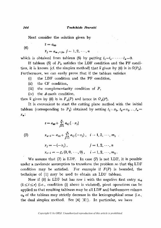
Next consider the solution given by
(6) Xj = a"'l+jo, j = 1,2, ... , n
which IS obtained from tableau (5) by putting t1=t2=··· =t,,=O. If tableau (5) of P k satisfies the LDF condition and the PF condi
tion, it is known (cf. the simplex method) that x given by (6) is in O(Pk).
Furthermore, we can easily prove. that if the tableau satisfies (i) the LDF condition and the PF condition, (ii) the CF condition, (iii) the complementarity condition of P, (iv) the LI-mesh condition,
then x given by (6) is in F A(P) and hence in 0 A{P), It is convenient to start the cutting plane method with the initial
tableau (corresponding to PI) obtained by setting t1=X1, t2 =X2, •• ,t .. =
X,,:
(7) n
x .. +.=aiO+I:aij(-Xj), i=I,2,···,m1 j-l
Xj=-(-Xj), j=I,2, ... ,n
X,+i = - gi (0,0, ···,0) , i = 1,2, ... , m 2 •
We assume that (7) is LDF. In case (7) is not LDF, it is possible under a moderate assumption to transform the problem so that th~ LDF
t·
condition may be satisfied. For example if F(P) is bounded, the technique of [IJ may be used to obtain an LDF tableau.
Now if (5) is LDF but has row i with the negative first entry aiO
(I ::;;.i::;;'r) (i.e., condition (i) above is violated), pivot operations can be applied so that resulting tableaus may be all LDF and furthermore column ao of the tableau may strictly decrease in the lexicographical sense (i.e., the dual simplex method. See [4J [5J). In particular, we have
Copyright © by ORSJ. Unauthorized reproduction of this article is prohibited.
Complementarg Convex Programming 145
(8) Z(l) ::?; Z(2) ::?; '" ::?; Z(k) ;2: ... ,
where z(k) is Qoo in the k-th tableau. After a finite number of pivot operations a tableau satisfying the PF condition results if it is feasible.
In the cutting plane method, a cut is generated if one of (ii) , (iii) and (iv) discussed above is not satisfied. The cut is written by
(9)
where
S::?;O
Po < 0,
in terms of the nonbasic variables t l , j = 1, 2, .. , n. After (9) added, a pivot operation is again incurred because (9) has the negative first entry Po. Now it is time to discuss three types of cuts corresponding to cases (ii) , (iii) and (iv).
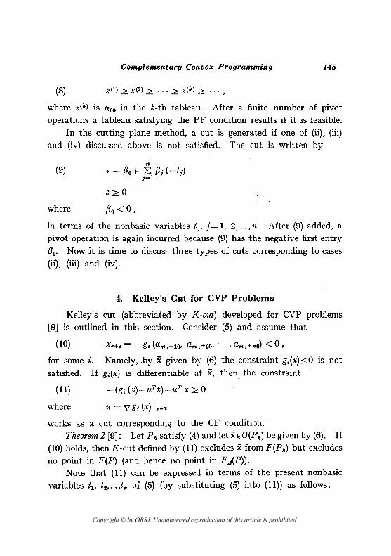
4. Kelley's Cut for CVP Problems
Kelley's cut (abbreviated by K-cut) developed for CVP problems [9] is outlined in this section. Consider (5) and assume that
(10) X,+j = - gj (a", ,+10' am ,+20' .. " a""+,,o) < 0 ,
for some i. Namely, by x given by (6) the constraint g;(x):::;:O IS not satisfied. If gj(x) is differentiable at X, then the constraint
(11)
where
-(gj (x)-UTX)-UT x::?; 0
u = V' gj (x) !s=%
works as a cut corresponding to the CF condition. Theorem 2 [9J: Let P k satisfy (4) and let XEO(Pk ) be given by (6). If
(10) holds, then K-cut defined by (11) excludes x from F(Pk) but excludes no point in F(P) (and hence no point in F ,d(P)).
Note that (11) can be expressed in terms of the present nonbasic variables t1, t2, •• ,t" of (5) (by substituting (5) into (11)) as follows:
Copyright © by ORSJ. Unauthorized reproduction of this article is prohibited.
146 Toshihide Ibaraki
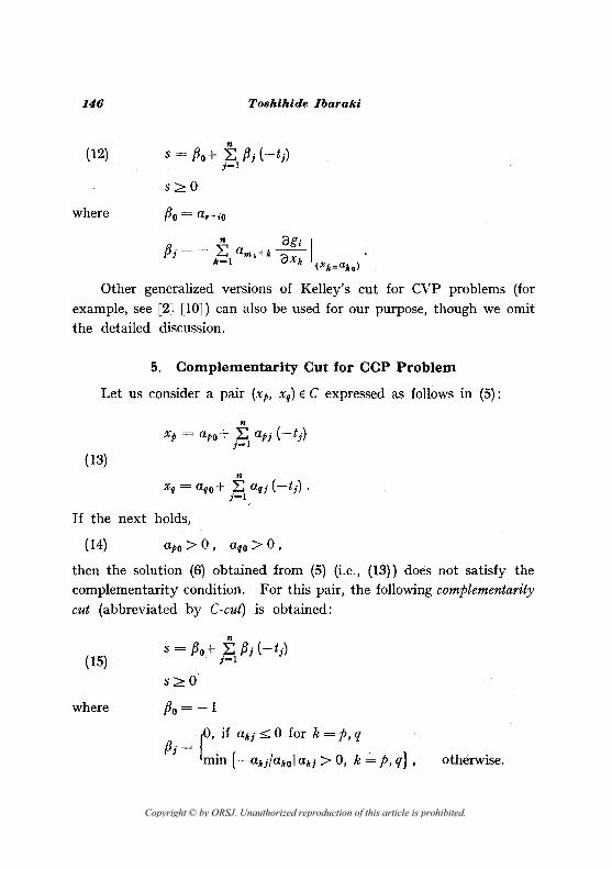
(12)
S20
where
Other generalized versions of KeUey's cut for CVP problems (for
example, see [2J [1OJ) can also be used for our purpose, though we omit the detailed discussion.
5. Complementarity Cut for CCP Problem
Let us consider a pair (xp, Xq) E C expressed as follows in (5):
(13)
If the next holds,
(14) apo>O, aqo>O,
then the solution (6) obtained from (5) (i.e., (13)) does not satisfy the complementarity condition. For this pair, the following complementarity
cut (abbreviated by C-cut) is obtained:
( 15)
where
S20
Po = -1
f>, if Ukj::;: 0 for k = P, q pj = L·
mm {-akj!akOI Ukj > 0, k = P, q} , otherwise.
Copyright © by ORSJ. Unauthorized reproduction of this article is prohibited.
Complementary Convex Programming 147
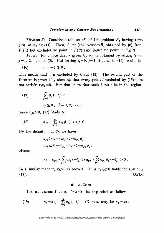
Theorem 3: Consider a tableau (5) of LP problem Plo having rows (13) satisfying (14). Then, C-cut (15) excludes X, obtained by (6), from
F(P,,) but excludes no point in F(P) (imd hence no point in F A(P)), Proof: First note that x given by (6) is obtained by letting t;="O,
j=l, 2, . . ,n, in (5). But letting tj=O, j=l, 2, . . ,n, in (15) results in
(16) s = -1 4: ° . This means that x is excluded by C-cut (15). The second part of the theorem is proved by showing that every point t excluded by (15) does not satisfy XpXg=O. For that, note that such t must be in the region
n (17) L:(3·(-t·)<1
j_1 J J
tf;z 0, j = 1,2, "', n .
Since IT{>o> 0, (17) leads to
(18)
By the definition of (31, we have
Hence
apj > 0 => apj ::;;: -apo (3j
ap!::;;: 0 => apj::;;: 0::;;: -al;o(3j.
In a similar manner, xq>O is proved. Thus XpXg>O holds for any t in QED. (In
6. A-Guts
Let us assume that Xi, O::;;:i::;;:r, be expanded as follows:
(19) n
Xi = aiO + ?: aij (-tj ). (Note Xi may be Xo = z) • J=I
Copyright © by ORSJ. Unauthorized reproduction of this article is prohibited.
148 Toshihide lbaraki
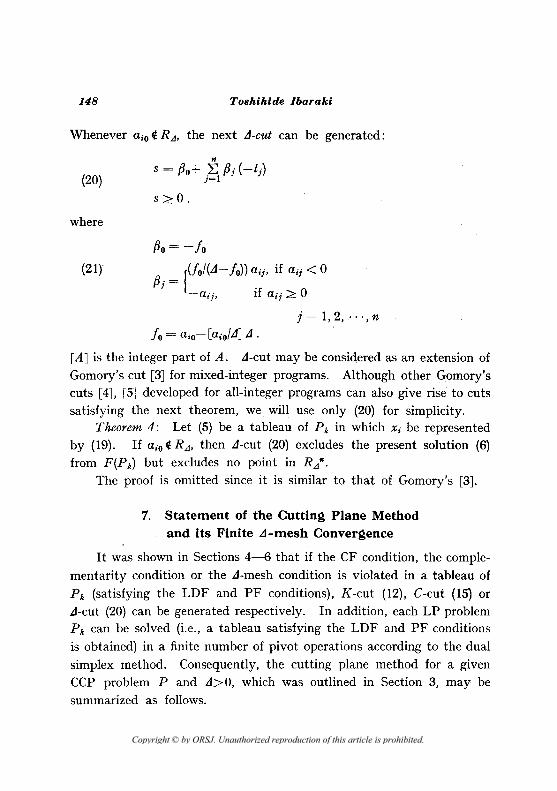
Whenever aiO It RA' the next ,1-cut can be generated:
(20)
where
(21)
s:;:::: O.
Po = -10
{(fo/(,1-10)} aij, if aij < 0 p. =
J -aij, if aij :;:::: 0
j=I,2, ... ,n
10 = aiO- [a,o/,1J ,1 .
[AJ is the integer part of A. ,1-cut may be considered as an extension of Gomory's cut [3J for mixed-integer programs. Although other Gomory's cuts [4J, [5J developed for all-integer programs can also give rise to cuts satisfying the next theorem, we. will use only (20) for simplicity.
Theorem 4: Let (5) be a tableau of P k in which Xi be represented by (19). If aiO It RA' then ,1-cut (20) excludes the present solution (6) from F(Pk} but excludes no point in RA".
The proof is omitted since it is similar to that of Gomory's [3].
7. Statement of the Cutting Plane Method and its Finite ,1-mesh Convergence
It was shown in Sections 4-6 that if the CF condition, the complementarity condition or the ,1-mesh condition is violated in a tableau of
P k (satisfying the LDF and PF conditions), K-cut (12), C-cut (IS) or ,1-cut (20) can be generated respectively. In addition, each LP problem P k can be solved (i.e., a tableau satisfying the LDF and PF conditions
is obtained) in a finite number of pivot operations according to the dual simplex method. Consequently, the cutting plane method for a given CCP problem P and ,1>0, which was outlined in Section 3, may be
summarized as follows.
Copyright © by ORSJ. Unauthorized reproduction of this article is prohibited.
Complementary Convex Programming 149
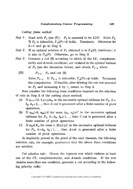
Cutting plane method:
Step 1: Start with P l (see (7)). PI is assumed to be LDF. Solve PI' If PI is infeasible, F ,d(P) =1> holds. Terminate. Otherwise let k=1 and go to Step 2.
Step 2: If an optimal solution of P k obtained is in F,d(P), terminate; it is also in O,d(P). Otherwise, go to Step 3.
Step 3: Generate a cut (9) according to which of the CF, complementarity and i1-mesh conditions, are violated in the optimal tableau of P k (see the discussion below), and obtain P k+l where
(22) P k+l: P k and cut (9).
Solve P k+1• If P k+ l is infeasible, F ,d(P) =1> holds. Terminate the computation. If feasible, after deleting the cut row annexed to P k and increasing k by 1, return to Step 2.
Now consider the following three conditions imposed on the selection of cuts in Step 3 of the cutting plane method.
(a) If a,+i<O, l::;:i::;:m2, in the successive optimal tableaus for Ph, k=
ko, ko+ 1, .. , then K-cut is generated after a finite number of pivot operations.
(b) If apo>O, ago>O for some (xl'> Xg) E C in the successive optimal tableaus for Pk, k=ko, ko+ 1, .. , then C-cut is generated after a finite number of pivot operations.
(c) If aio ft R,d for some i, (O:O;::i::;:r} in the successive optimal tableaus
for Pk, k=ko, ko+ 1, .. , then i1-cut is generated after a finite number of pivot operations.
As implicitly proved in the proof of the next theorem, the following selection rule, for example, guarantees that the above three conditions are satisfied.
Cut selection rule: Choose the topmost row which violates at least one of the CF, complementarity, and i1-mesh conditions. If the row violates more than one condition, generate a cut accOIding to the follow
ing priority order.
Copyright © by ORSJ. Unauthorized reproduction of this article is prohibited.
150 Toshihide Ibaraki
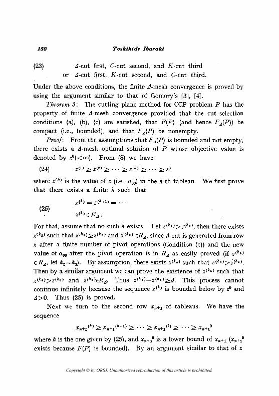
(23) LI-cut first, C-cut second, and K-cut third or LI-cut first, K-cut second, and C-cut third.
Under the above conditions, the finite A-mesh convergence is proved by using the argument similar to that of Gomory's [3J, [4].
Theorem 5: The cutting plane method for CCP problem P has the property of finite LI-mesh convergence provided that the cut selection conditions (a), (b), (c) are satisfied, that F(P) (and hence F A(P)) be compact (i.e., bounded), and that FA(P) be nonempty.
Proof: From the assumptions that F A(P) is bounded and not empty, there exists a LI-mesh optimal solution of P whose objective value is denoted by i'«oo). From (8) we have
(24) Z(l) ::?: Z(2) ::?: •.• :;;:: Z(k) ::?: ... ::?: ZO
where Z(k) is the value of z (i.e., aoo) in the k-th tableau. We first prove that there exists a finite k such that
(25) Z(k) E RA •
For that, assume that no such k exists. Let z(kd>z(k.), then there exists z(k g ) such that z(kl)::?:Z(k.) and z(k.) ERA, since LI-cut is generated from row
z after a finite number of pivot operations (Condition (c)) and the new value of aoo after the pivot operation is in RA as easily proved (if Z(k.)
E RA, let k2=k3). By assumption, there exists z(k.) such that z(k·»i(k.).
Then by a similar argument we can prove the existence of Z(k,) such that Z(kl»Z(k,) and z(k·)ERA• Thus Z(kl)-Z(k'):;;::LI. This process cannot continue infinitely because the sequence z(k) is bounded below by i' and LI>O. Thus (25) is proved.
Next we turn to the second row X,,+l of tableaus. We have the
sequence
X"+l(k):;;:: X"+l(k+1):;;:: ••• :;;:: X"+l(l):;;:: ••• :::: x .. +1o
where k is the one given by (25), and X"+lO is a lower bound of X"+l (X"+lO
exists because F(P) is bounded). By an argument similar to that of z
Copyright © by ORSJ. Unauthorized reproduction of this article is prohibited.
Complementary Con.vex Programming
we can prove that after a finite number t,
is satisfied.
X n+1 (I) = X n+1 (I +1) = ...
Xn+1 (1) E R,:j
151
Applying this argument to X n+ 2 •.. ,X"+,,, l' Xl' .. , Xn successively, we will see that after a finite number of pivot operations,
X(S) = X(S+l) = ...
x(S)ER,:j"
holds. x(S) must be in F,:j(P) , since otherwise K-cut or C-cut must be generated after a finite number of pivot operations and it provides a
new different solution, contradicting the fact that X has converged to x(s). Also, x(S) must be in O,:j(P) because F(Pu)~F,:j(P) from the defini
tion of cuts, where the s-th tableau is generated for LP problem Pu .
QED. Although conditions (a), (b) and (c) are introduced to guarantee the
finite convergence, other selection rules sometimes may prove effective
in speeding up the convergence. For example the following rule appears reasonable that selects C-cuts or K-cuts first, until the improvement in the objective values becomes very small, and then relies on i1-cuts. After an appropriate number of Lt-cuts, C-cuts or K-cuts are again generated, and the process is repeated.
8. Example
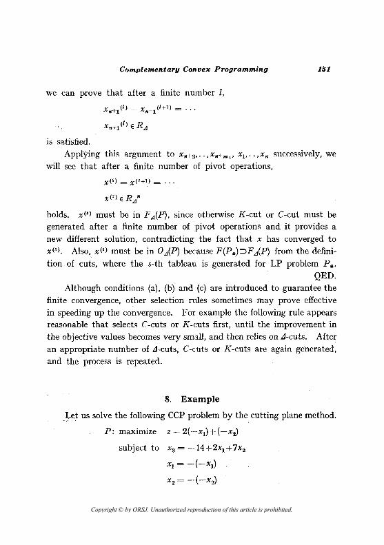
L~t us solve the following CCP problem by the, cutting plane method.
P: maximize z = 2(--x1) + (-x2)
subject to X3= --14+2X1+7X2
Xl = -(-Xl)
X2 = --(-X2)
Copyright © by ORSJ. Unauthorized reproduction of this article is prohibited.
152 Toshihide lbaraki
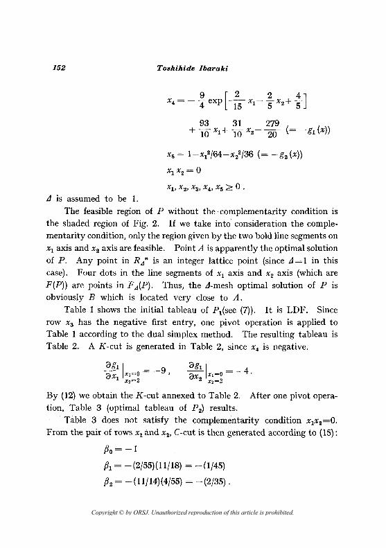
x = - ~ exp [_2_ x - ~ x + ..!] 4 4 15 I 5 2 5
LI is assumed to be 1.
The feasible region of P without the· complementarity condition is the shaded region of Fig. 2. If we take into consideration the complementarity condition, only the region given by the two bold line segments on Xl axis and X2 axis are feasible. Point A is apparently the optimal solution of P. Any point in RA" is an integer lattice point (since LI = 1 in this case). Four dots in the line segments of Xl axis and X2 axis (which are F(P)) are points in FA(P). Thus, the LI-mesh optimal solution of P is obviously B which is located very close to A.
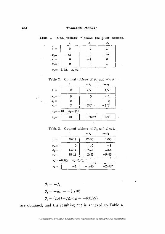
Table 1 shows the initial tableau of PI(see (7)). It is LDF. Since row Xa has the negative first entry, one pivot operation is applied to Table 1 according to the dual simplex method. The resulting tableau is Table 2. A K-cut is generated in Table 2, since X4 is negative.
By (12) we obtain the K-cut annexed to Table 2. After one pivot operation, Table 3 (optimal tableau of P 2) results.
Table 3 does not satisfy the complementarity condition X IX2=O.
From the pair of rows Xl and X2, C-cut is then generated according to (15):
Po = -1
PI = - (2/55){1l/18) = - 0/45)
P2 = - (11/14)(4/55) = - (2/35) .
Copyright © by ORSJ. Unauthorized reproduction of this article is prohibited.
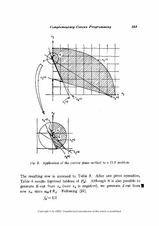
Complementary Convex Programming 153
Fig. 2. Application of the cutting plane method to a CCP problem.
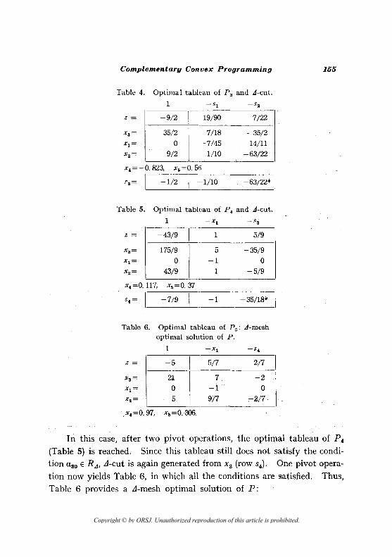
The resulting row is annexed to Table 3. After one pivot operation, Table 4 results (optimal tableau of P 3). Although it is also possible to generate K-cut from X 4 (note X 4 is negative), we generate J-cut fromll
row X2' since a30 ft RA. Following (21),
10'= 1/2
Copyright © by ORSJ. Unauthorized reproduction of this article is prohibited.
154 Toshihide Ibaraki
Table 1. Initial tableau; * shows the pivot element.
1
Z= 0 1 2 1
-14 -2 -7* 0 -1 0 0 0 -1
Table 2. Optimal tableau of PI and K-cut.
1 -Xl -X3
Z= -2
0 0 2
x.=-lO, x5=8/9
Sl= I -10
1 12/7 1/7
0 -1 ~l 0
2/7 -1/7
-55/7* -4/7
Table 3. Optimal tableau of P 2 and C-cut.
1 -Sl -X3
Z= -46/11 I 12/55 1/55
0 .0 -1
14/11 -7/55 4/55 18/11 2/55 -9/55
"
X.=-0.05, xli=0.61 S2 = 1-----1---.1 ---1-/4-"5-;""":"""'---2-/3-5-*-1
Po = - fo
PI = -aS1 = -(1/10)
P2 = Uo/(I- fo)) aS2 = -(63/22)
are obtained, and the resulting cut is annexed to Table 4.
Copyright © by ORSJ. Unauthorized reproduction of this article is prohibited.
Complementary COn1Jex Programming
Table 4. Optimal tableau of P a and A-cut.
1 -51 -52
Z= -9/2 19/90
Xl = 0 -7/45 X 2= 9/2 1/10
7/22
-35/2 14/11
-63/22
Xa= ~35/2 7/18
----------, x,=-0.823, x.=O.56
sa = 1 -1/2 _.-1-/1-0-----6-3/-2-2*-1
Table 5. Optimal tableau of p. and A-cut.
1 -Xl -Sa
Z= -43/9 1 5/9
X3= 175/9 5 -35/9 x l = 0 -1 0 x2 = 43/9 1 -5/9
x.=0.117, x.=0.37
5.= I -7/9 -1 -35/18* 1
Table 6. Optimal tableau of p.: A-mesh optimal solution of P.
1 -Xl -5.
Z= -5 5/7 2/7
X3= 2,1. 7 -2 x l = 0 -1 0
x.= 5 9/7 .,-217 -
-,x.=0.97, x5=0.306
155
In this case, after two pivot operations, the optimal tableau of P 4
(Table 5) is reached. Since this tableau still does not satisfy the condition a30 ERA, J-cut is again generated from X 2 (row S4)' One pivot operation now yields Table 6, in which all the conditions are satisfied. Thus, Table 6 provides a J-mesh optimal solution of P:
Copyright © by ORSJ. Unauthorized reproduction of this article is prohibited.
156 Toshihide Ibaraki
Z= -5
Xl = O. x 2 = 5.
The trajectory of solutions obtained for PI> P 2 •• • • p s is also illustrated in Fig. 2.
Note that. however. the solution of Table 5 is also incidentally
feasible in p. though aao tt RA' Thus if we terminated the computation at this stage. a better solution
Z = -(43/9)
X 2 = 43/9
would have been obtained. Although this situation does not always
occur. it will provide a better solution than the .:I-mesh optimal solution.
9. Relation between .:I-mesh Optimal Solutions
and Optimal Solutions
The selection of .:I plays a crucial role in the cutting plane method.
If the value of .:I is too large. the displacement from the real optimal
solution of P could be intolerable. whereas if .:I is too small. the conver
gence speed would be slow. The next theorem relates the size of .:I with the accuracy of .:I-mesh optimal solution: .:I-mesh optimal solution can
come arbitrarily close to some optimal solution of P if an appropriate .:I
is chosen.
Let x E O{P) and ] (x) c {I. 2 •...• r} be such that
(a) j E](X) implies Xj = O. and
(b) either p or q E] (x) for every (xp. Xq) E C . (26)
We define that CCP problem P has C-interior if P has x E O{P). ](x) and
x E R" such that
X'*X = O. if k E]{X)
Xk { :;:::O.ifktt]{x). k=I.2.···.n
Copyright © by ORSJ. Unauthorized reproduction of this article is prohibited.
Complementary Convex Programming 157
(27)
i=1,2,···,ml
X,+. = -g. (Xl' X2, ••• , _i,,) > 0, i = 1,2, ... , m z .
Theorem 6: Let us assume that coefficients of CCP problem Pare all integers, F(P) is compact and P has C-interior. Let X.d stand for a J-mesh optimal solution of P. Then for any E>O, there exists .1 such that II~-x.dll ::::E. Furthermore there exists a sequence .11, .12" • ,Jk , • • such that Hm X.dk E O(P).
k-+oo
Proof: Let x E O(P), ](x) and x be defined by (26) and (27). Let H be the set of x E RIO such that
=O,ifjE](x)
xd:e:o, if jf](x), j== 1,2, ···,n
X,,+. {
= 0, if n+i E] (x)
:e:O, if n+i f](X), i= 1,2, ···,ml
X,+i = -gi (x) > 0, i=1,2,···,m2 •
H is nonempty (by assumption), convex and HcF(P). Now, for xEH, x(A.)=Xi+(1-X)~, 1:e:X>0, is also in H since H is convex.
Let B.(x(A.))={YEHI IIy-x(X)II<E}. Then for each A. and e it is
possible to select .1 such that
(28) B. (x(X)) n RA" *' cp i.e., B. (x(X)) n F.d (P) *' cp •
(By assumption on P, there exists XE:F(P) n B.(x("-)), whose components Xi, i = 1, 2, .. ,n, are all rational numbers. Then let .1 be any positive number satisfying 1/.1: integer and x,/J: integer for i=1, 2, .. , n.) Obviously any x'EB.(x(X))nRA" satisfies z(x):e:z(X.d):e:z(x'). Now for each A.k, k= 1, 2, .. , such that Hm "-k'=O, we can choose Ek and J k satisfy-
k-+oo
Copyright © by ORSJ. Unauthorized reproduction of this article is prohibited.
158 Toshihide lbaraki
ing (28) and lim ck =0. Thus lim X(Xk) =x and hence lim lim x' =X k-.cJO k-+co Ak-O! k-O
imply that z(x) =lim z(X.::Ik)' lim X.::Ik EF(P) follows from the compactness k-+oo k-oo
of F(P). (Even if this limit does not exist, we can choose a subsequence {..1 j } of {..1d so that X.::Ij has a limit, since F(P) is compact. Then {..1;} may be regarded as the sequence t.1d.) This proves the second half of the theorem. The first half immediately follows from the second half.
QED. From this theorem, we see that the sequence of ..1 j ' j=l, 2, .. , for
example such that .1j =IJj always contains a subsequence {..1k} having the property lim X.::Ik E O(P). .
k-oo
10. Discussion
When problem P has no convex constraint (i.e., 1#2=0), P is called a complementary linear programming (CLP) problem. In this case, the cutting plane method is considerably simplified; o~ly C-cuts and ..1-cuts are required to carry out the computation. This is a great saving
because K-cut requires the differentiation of g. which is quite time consuming.
Another advantage is that an exact optimal solution can be obtained , ,'.'., ,
by the cutting plane method if we choose an appropriate value of ..1. As proved in [6J, there exists ..1 such:that
(29) F.::I (P) n O(P) =1= 1>
for each ctp problem, under the· assumption that coefficients are all
rational numbers (This follows from the fact that there exists XEO(P) which is also a basic solution of Q and that there exists only a finite number of basic solutions). Therefore if we use ..1 satisfying (29) and
apply the cutting plane method, the resulting ..1-mesh optimal solution is also an optimal solution of P. The calculation of .1 of (29), however, is not easy for most of CLP problems. 'Thus it is difficult to consid~r this
Copyright © by ORSJ. Unauthorized reproduction of this article is prohibited.
Complementary Conl'ex Programming 159
approach as a practical method applicable to all CLP problems. In some
cases such as CLP problems with unimodular coefficient matrices, however, it is trivial to calculate J satisfying (29) and. the cutting plane
method may be used to obtain an exact optimal solution. Finally, note that our method can also be applied to CVP problems
which do not have the complementarity condition. It still has the property of finite J-mesh convergence. This makes a contrast with the conventional cutting plane methods for CVP problems [9J, [IOJ, none of which has the property of finite convergence.
Acknowled~ment
The author wishes to express his appreciation to Prof. H. Mine of Kyoto University for his support and. valuable comments on the study. He is also indebted to one of the referees who has suggested a shorter
proof of Theorem 3, which is adopted in this revision.
References
[1] Dantzig, G.B., L.R. Ford, and D.R. Fulkerson, "A Primal-Dual Algorithm for Linear Programs," in Linear Inequalities and Related Systems, H.W. Kuhn and A.W. Tucker (eds.), Princeton University Press, Princeton, 1956.
[2] Eaves, B.C. and W.!. Zangwill, "Generalized Cutting Plane Algorithms," Technical Report, Department of Operations Research, Stanford University, 1969.
[3] Gomory, R.E., "An Algorithm for the Mixed Integer Problem," P-1885, The RAND Corp. Inc., 1960.
[4] Gomory, R.E., "An Algorithm for Integer Solutions to Linear Programs," in Recent Advances in Mathematical Programming, R.L. Graves and P. Wolfe (eds.), McGraw-Hill, New York, 19G3.
[5] Gomory, R.E., "An All-Integer Integer Programming Algorithm," in Industrial Scheduling, J.R. Muth and G. L. Thompson (eds.). Prentice-Hall, 1963.
[6] Ibaraki, T., "Complementary Progracnming," (in Japanese) Keiei Kagaku, 16 (1972), 33-51.
[7] Ibaraki, T., "Complementary Programming," OPerations Research, 19 (1971), 1523-1529.
Copyright © by ORSJ. Unauthorized reproduction of this article is prohibited.
160 Toshihide Ibaraki
[8] Ibaraki, T., "The Use of Cuts in Complementary Programming," to appear in Contributions to Programming and Applications, E. Balas, R.W. Cottle, T.C. Hu and M.J.L. Kirby (eds.), ORSA, 1973.
[9] Kelley, J.E., Jr., "The Cutting-Plane Method for Solving Convex Programs," J. of SIAM, 8 (1960), 703-712.
[10] Topkis, D.M., "Cutting-Plane Methods without Nested Constraint Sets," Operations Research, 18 (1970), 404-413.
Copyright © by ORSJ. Unauthorized reproduction of this article is prohibited.