1

Anomaly testingJames Theiler

Space Data Science and Systems GroupLos Alamos National Laboratory

Abstract

An anomaly is something that in some unspecified way stands out from its background, and thegoal of anomaly testing is to determine which samples in a population stand out the most. This chapterpresents a conceptual discussion of anomalousness, along with a survey of anomaly detection algorithmsand approaches, primarily in the context of hyperspectral imaging. In this context, the problem can beroughly described as target detection with unknown targets. Because the targets, however tangible theymay be, are unknown, the main technical challenge in anomaly testing to characterize the background.Further, because anomalies are rare, it is the characterization not of a full probability distribution butof its periphery that most matters. One seeks not a generative but a discriminative model, an envelopeof unremarkability, the outer limits of what is normal. Beyond those outer limits, hic sunt anomalias.

CONTENTS

I Introduction 2I-A Anomaly testing as triage . . . . . . . . . . . . . . . . . . . . . . . . . . . 2I-B Anomalies drawn from a uniform distribution . . . . . . . . . . . . . . . . 2

I-B1 Nonuniform distributions of anomalousness . . . . . . . . . . . 4I-C Anomalies as pixels in spectral imagery . . . . . . . . . . . . . . . . . . . 4

I-C1 Global and local anomaly detectors . . . . . . . . . . . . . . . 5I-C2 Regression framework . . . . . . . . . . . . . . . . . . . . . . . 6

II Evaluation 6

III Periphery 7

IV Subspace 9

V Kernels 10V-A Kernel density estimation . . . . . . . . . . . . . . . . . . . . . . . . . . . 10V-B Feature space interpretation: the “kernel trick” . . . . . . . . . . . . . . . 10

VI Change 13VI-A Subtraction-based approaches to anomalous change detection . . . . . . . 13VI-B Distribution-based approaches to anomalous change detection . . . . . . . 15VI-C Further comments on anomalous change detection . . . . . . . . . . . . . 16

VII Conclusion 16

Appears as: Chapter 19 in Statistical Methods for Materials Science: The Data Science of MicrostructureCharacterization, J. P. Simmons, C. A. Bouman, M. De Graef, and L. F. Drummy, Jr., eds. (CRC Press, 2018).ISBN 9781498738200.

2

I. INTRODUCTION

Traditionally, anomalies are defined in a negative way, not by what they are but by what theyare not: they are data samples that are not like the data samples in the rest of data. “There isnot an unambiguous way to way to define an anomaly,” one review notes, and then goes onto ambiguously define it as “an observation that deviates in some way from the backgroundclutter” [1]. Anomalies are defined “without reference to target signatures or target subspaces”and “with reference to a model of the background” [2]. Indeed, as Ashton [3] remarks, “thebasis of an anomaly detection system is accurate background characterization.”

This exposition will concentrate on anomaly detection in the context of imagery, with particularemphasis on hyperspectral imagery (in which each pixel encodes not the usual red, green, andblue of visible images, but a spectrum of radiances over a range of wavelengths that oftenincludes upwards of a hundred spectral channels). Testing for anomalies is an exercise thathas application in a variety of scenarios, however. Since anomalies are deviations from what isnormal, particularly in situations where the nature of that deviation is not be predictable or wellcharacterized, anomaly detection has been used in a variety of fault detection contexts [4]–[8].

What we are calling anomaly testing here is essentially the same as what the machine learningcommunity calls “novelty detection” [9]–[11] or “one-class classification” [12], [13].

A. Anomaly testing as triageAlthough we may have difficulty defining anomalies, the reason we seek them is that (being

rare and unlike most of the data) they are potentially interesting and possibly meaningful. Wehave to acknowledge that “interesting” is even harder to define than “anomalous” but in thisexposition, we will make this distinction, partly because it separates the mystical “by definitionundefined” [14] aspect of the interesting-data detection problem into two components, whichcorrespond to the two boxes in Fig. 1.

We can indeed define “anomalous,” but will leave “interesting” and “meaningful” to be domain-specific concepts. From this point of view, anomaly detection is a kind of triage. If anomaliescan be defined and detected in a relatively generic way, then experts in the specific area ofapplication can decide which anomalies are interesting or meaningful.

Here the goal of anomaly detection is to reduce the quantity of incoming data to a level thatcan be handled by the more expensive downstream analysis. It is this later analysis that judgeswhich of the anomalous items are in fact meaningful for the application at hand. This judgmentcan be very complicated and domain-specific, and can involve human acumen and intuition.What makes anomaly detection useful as a concept is that the anomaly detection module hasmore generic goals, and is consequently more amenable to formal mathematical analysis.

B. Anomalies drawn from a uniform distributionAnomalies are rare, and where we expect to find them is in the far tails of the background

distribution pb(x). We can express “anomalousness” as varying inversely with with this densityfunction, and can derive this expression in two distinct ways, each providing its own insight.

In the first and most direct approach, we make an explicit generative model for anomalies,and say that they are samples drawn from a uniform distribution. This is a simple statement, butit is in some ways revolutionary; in contrast to conventional wisdom [1]–[3], we are defininganomalies directly, without respect to the background distribution. To distinguish these anomaliesfrom the background, we treat the detection as a hypothesis testing problem. The null hypothesis

3

Interesting

AnomalyDetector

DataAnomalous

Data

Some kind offurther analysis

Data

Fig. 1. Anomaly testing as triage. In this picture, anomaly detection provides a way to reduce the raw quantity of data thatneeds to be considered by further analysis. That further analysis might be expensive domain-specific automated processing, orit may involve human inspection, with trained analysts making judgments about whether the potentially interesting anomaly isindeed interesting or meaningful or important.

is that the measurement x is drawn from the background distribution (x = z with z ∼ pb), andthe alternative hypothesis is that x is drawn from the anomalous distribution (x = t with t ∼ u).This leads to the likelihood ratio

L(x) = P (x = t)

P (x = z)=

u(x)

pb(x)=

c

pb(x)(1)

where u(x) = c is the uniform distribution from which anomalies are drawn.1 The expressionin Eq. (1) is a candidate for “anomalousness” because a large value of L(x) indicates a higherlikelihood that x is drawn from the anomalous distribution.

In the second approach, we avoid making an explicit model of what an anomaly is, but weassume that the effect of the anomaly on the scene is additive. In particular, we say that a pixelwith an anomaly in it is of the form x = z + t where t is the unknown target, and z is thebackground. We employ the generalized likelihood ratio test to write

L(x) = P (x = z+ t)

P (x = z)=

maxt pb(x− t)

pb(x)=

maxz pb(z)

pb(x)=

c′

pb(x)(2)

where the (again, irrelevant) constant c′ is the maximum value of pb and does not depend on x.This second approach produces the same result as the first, but the argument used to get thatresult has two problems: one, the additive assumption is very restrictive and may not apply tothe scenario of interest; and two, it uses a generalized likelihood ratio test (GLRT). Althoughthe GLRT is a popular and often practical tool, it has ambiguous properties, and can producedetectors that are not only sub-optimal, but in some cases inadmissible [16], [17]. This is not tosay that the detector in Eq. (2) is inadmissible; indeed, it is identical to the detector in Eq. (1).The objection is not to the detector but to this second derivation of the detector via the GLRT. Asupposed advantage of this second derivation is that it makes “no assumptions” about the natureof the anomaly, but this is a spurious argument. In fact, it is making implicit assumptions aboutthe distribution of an anomaly, but it is not providing the algorithm designer with access to alterthose implicit assumptions.

Although there are many reasons to favor the first approach, it is the second argument that ismost widely invoked in the hyperspectral anomaly detection literature.

1The constant c is irrelevant to our purposes, and in fact it is possible to make this argument in a more formal way that treatsu(x) not as a proper probability distribution, but more generally as a measure [15].

4

We remark that the first approach can also accommodate additive anomalies. Here, the nu-merator of the likelihood ratio is a Bayes factor, but it still evaluates to a constant independentof x:

L(x) = P (x = z+ t)

P (x = z)=

∫pb(x− t)u(t)dt

pb(x)=c∫pb(z)dz

pb(x)=

c′′

pb(x)(3)

We again obtain the result that anomalousness varies inversely with pb(x), the probability densityfunction of the background. Contours of anomalousness will be level curves of the backgrounddensity functions. For a Gaussian distribution, these contours are ellipsoids of constant Ma-halanobis distance [18], with larger distances corresponding to smaller densities and greateranomalousness; we can therefore use Mahalanobis distance as a measure of anomalousness

A(x) = (x− µ)TR−1(x− µ) (4)

where µ is a vector-valued mean and R is a covariance matrix.The Mahalanobis distance is the basis of the Reed-Xiaoli (RX) detector [19]–[21]. Although

RX, as originally introduced [19], refers specifically to multispectral imagery, and in fact is alocal anomaly detector, the term “RX” is often used as a shorthand for Mahalanobis distancebased anomaly detection.

1) Nonuniform distributions of anomalousness: Since the assumption of a uniform distributionfor anomalies is explicit in the derivation of Eq. (1) – and by extension, Eq. (4) – that allows us toconsider other, nonuniform, distributions if we are looking for other kinds of anomalies. Examplesinclude anomalous change (to be further discussed in Section VI), and anomalous “color” inmultispectral imagery. Here, in place of a uniform distribution of anomalies, a distribution ofanomalously colored pixels are generated from the product of marginal distributions associatedwith each individual spectral band. To sample at random from this distribution, one creates avector-valued pixel where each component is independently sampled from the correspondingcomponent of the multispectral image [22].

Another example is given by the blind gas detection algorithm. In the traditional gas detectionproblem, one is looking for plumes that contain a gas-phase chemical of interest. When theabsorption spectrum of that chemical of interest is known, one can derive a matched filter thatcan detect impressively low concentrations of the chemical [23]. In the blind gas detectionproblem, one does not have a single chemical (or even a short list of chemicals) of interest; onewants to detect chemical plumes without knowing the chemical species in the plume. But onedoes know that gas-phase chemicals usually have very sparse spectral signatures – i.e., there iszero or nearly-zero absorption at all but a few wavelengths. A sparse RX (or “spaRX”) algorithmwas developed for detecting spectrally sparse additive anomalies t based on the RX derived inEq. (2), but with t constrained to a limited number of nonzero components [24].

C. Anomalies as pixels in spectral imageryTraditional statistical analysis treats data as a set of discrete samples that are drawn from a

common distribution. Because each pixel in a hyperspectral image contains so much information(a many-channel spectrum of reflectances or radiances), one can often quite profitably treat thepixels as independent and identically distributed. It is as if the image were a “bag of pixels.” Buthowever spectrally informative individual pixels are, they comprise an image, and the spatialstructure in an image provides further leverage for characterizing the background and discoveringanomalies.

5

Hyperspectral imagery provides a rich and irregular data set, with complex spatial and spectralstructure. And the more accurately we can model this cluttered background, the better ourdetection performance. Simple models can be very effective, but the mismatch between simplemodels and the complicated nature of real data has driven research toward the development ofmore complex models [25].

1) Global and local anomaly detectors: A pixel is anomalous in the context of a background.In global anomaly detection that background is the full image, but in local anomaly detectionthat background restricted to the immediate neighborhood, often defined in terms of an annulusthat surrounds the pixel. Local anomaly detection is one of the most straightforward (and, inpractice, more effective) ways to exploit the spatial structure of imagery.

Indeed, the initial formulation of the RX algorithm [19] computed anomalousness at eachpixel in terms of a local mean and a local covariance matrix, each computed from the pixelsin an annulus surrounding that pixel. The trade-off in choosing the size of the annulus is thata larger annulus will have better “statistics” – since it has more pixels, it will better averageout the fluctuations in the pixels values; but a smaller annulus will be less affected by spatialnonstationarity [26]. Matteoli et al. [1] observed that one could use a smaller annulus for thelocal mean and a larger annulus for the local covariance. This is very sensible, since the need for“good statistics” is greater for the covariance matrix than for the mean vector. As the covarianceannulus approaches the size of the image, this approach can be simplified by using a local meanand a global covariance, but with the global covariance based on subtraction of the spatiallyvarying local mean. A broad survey of approaches used to improve estimates of local covariance,including regularization, segmentation, and robustification, is provided by Matteoli et al. [27].

The importance of regularization derives from the fact that RX requires the inverse of thecovariance matrix. If the covariance matrix is singular, then the inverse does not exist, andregularization is required. But even for a well-conditioned covariance matrix, the best estimator ofthe inverse is not the same as the inverse of the best estimator, and some amount of regularizationis still beneficial. The most common and straightforward regularization is by shrinkage. Here,we estimate the covariance matrix with a linear combination of the sample covariance Rs (whichtends to overfit the data) and a very simple estimator Ro that tends to underfit the data

R = (1− α)Rs + αRo (5)

where typically α � 1. In the simplest case, Ro is just a multiple of the identify matrix [28],[29] (choosing the multiple so that Ro has trace equal to Rs ensures that α is dimensionless).An argument can be made for shrinkage against the diagonal matrix [30], [31], an approach thatis generalized in the sparse matrix transform [32], [33]. Caefer et al. [34] recommended a quasi-local estimator that combines local and global covariance estimators by using local eigenvalueswith global eigenvectors.

The idea of segmentation is to replace the moving window with a static segment of similarpixels that surround the pixel of interest in a more irregular way. Here the image is partitionedinto distinct segments of (usually contiguous) pixels, and a pixel’s anomalousness is based onthe mean and covariance of the pixels in the segment to which the pixel belongs [34], [35]. Thissometimes leads to extra false alarms on the boundaries of the segments, and one way to dealwith this problem is with overlapping segments [36].

The estimation of covariance in the local annulus can be corrupted by one or a few outliers2and2Outliers and anomalies are essentially the same thing, and we make no formal distinction between them. But informally we

think of anomalies as rare nuggets deserving of further analysis, while outliers are nuisance samples that contaminate the dataof interest.

6

robust estimates of covariance [37]–[39] exclude or suppress the outliers in the computation.Excluding outliers is advisable in global estimates of covariance as well [40], [41].

2) Regression framework: By estimating what the target-free radiance should be at a pixel,we have a point of comparison with what the measured value of that pixel actually happensto be. It is common to make this estimate using the mean of pixels in an annulus around thepixel of interest. But there is more information in the annulus than this mean value [42], [43],and that suggests using more general estimators than just the mean. The derivation in [44] usesmultivariate regression of the central pixel against the pixels in the surrounding annulus. Thiscan be done on a band-by-band basis, or with multiple bands simultaneously. Other variants usemedian instead of mean [45], and a patch-based nearest neighbors regressor was also developed[46].

It is worth noting that the problem of estimating a central pixel, using the specific pixels thatimmediately surround it, along with the statistical context of the rest of the image, is a specialcase of the “inpainting” problem. In this case, only a single pixel is being inpainted at a time,but this inpainting is done for every pixel in the image.

II. EVALUATION

A conceptual problem with anomaly detection is the ambiguous nature of “interestingness.”But a more technical problem is that, since anomalies are by definition rare, it is difficult to findenough of them to do statistical comparisons of algorithms, and it is easy to be misdirected byanecdotal results.

Section I-B described how to resolve the ambiguity issue by treating anomalies as samples froma specific and well-defined, yet very broad and flat (e.g., uniform), distribution. This resolutionled, for instance in Eq. (1), to likelihood-based algorithms for anomaly detection.

An arguably more important advantage to treating anomalies as samples from a distributionis that it leads to a direct quantitative way to measure the performance of an anomaly detectionalgorithm, without relying on anecdotally identified anomalies in a given scene. The moststraightforward way of exploiting this model is to use it to create artificial targets that canbe “implanted” into the scene [26], [47]. This is usually performed at a judiciously chosensubset of locations, to avoid contaminating the background estimation with an unrealisticallylarge number of targets. But in some cases one can more efficiently place a target at effectivelyevery location in the image, producing matched pairs of with-target and without-target pixelsfrom which to learn a target detector [48].

An advantage of explicit implanting is that it can be made as realistic as the simulationwill allow. A potential disadvantage is that this explicit simulation can be expensive, mayrequire ad hoc choices. Particularly for anomaly detection, where physical properties of thetarget are generally not well known, or at least not well specified, more generic approaches maybe desirable.

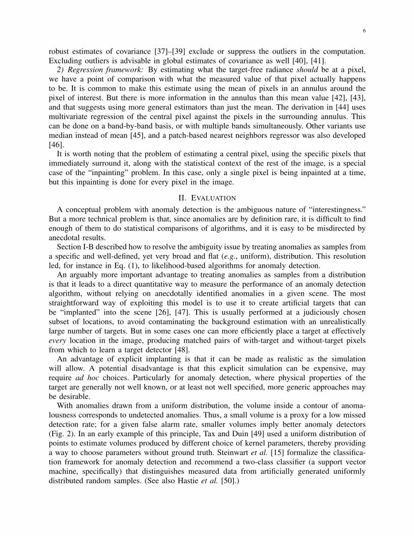
With anomalies drawn from a uniform distribution, the volume inside a contour of anoma-lousness corresponds to undetected anomalies. Thus, a small volume is a proxy for a low misseddetection rate; for a given false alarm rate, smaller volumes imply better anomaly detectors(Fig. 2). In an early example of this principle, Tax and Duin [49] used a uniform distribution ofpoints to estimate volumes produced by different choice of kernel parameters, thereby providinga way to choose parameters without ground truth. Steinwart et al. [15] formalize the classifica-tion framework for anomaly detection and recommend a two-class classifier (a support vectormachine, specifically) that distinguishes measured data from artificially generated uniformlydistributed random samples. (See also Hastie et al. [50].)

7

Fig. 2. Three anomaly detectors with the same false alarm rate (Pfa = 0.001). The contour marks the boundary between whatis normal (inside) and what is anomalous (outside). If anomalies are presumed to be uniformly distributed, then the anomalydetector with smallest volume will have the fewest missed detections.

Plotting volume (or log-volume, which is often more convenient, especially in high dimen-sions) against false alarm rate provides a ROC-like curve that characterizes the anomaly detector’sperformance [51], [52].

For a covariance matrix, the volume is proportional to the determinant of the matrix. For localanomaly detectors described in Section I-C1, one can still use a global covariance based onthe difference between measured and estimated (e.g., by local mean) values at each pixel, andthe smaller that covariance, the better the estimator. A natural choice, from a signal processingperspective is the total variance of that difference,∑

n

(xn − xn)T (xn − xn) (6)

which corresponds to the trace of the covariance matrix. Smaller values of this variance implythat x is closer to x, but Hasson et al. [45] point out that, in terms of target and anomalydetection performance, closer is not necessarily better.

When, instead of a global covariance estimator, we use a separate covariance for each pixel,based on the local neighborhood of that pixel, then it is more complicated. It is clear that thevolumes of the individual covariances should be small, but it is not obvious how best to combinethem. In Bachega et al. [53], it is argued, more on practical than theoretical grounds, that anaverage of the log volume is a good choice.

III. PERIPHERY

For anomaly detection, low false alarm rates are imperative. So the challenge is to characterizethe background density in regions where the data are sparse; that is, on the periphery (or “tail”)of the distribution. Unfortunately, traditional density estimation methods, especially parametricestimators (e.g., Gaussian), are dominated by the high-density core. And it bears pointing outthat “robust” estimation methods (e.g., [37], [54], [55]) achieve their robustness by paying evenless attention to the periphery.

Robustness to outliers can be achieved by essentially removing the outliers from the data set.This direct approach is taken by the MCD (Minimum Covariance Determinant) of Rousseeuw etal. [37], [55]. For a data set of N samples, the idea is to take a core subset H of h < N samplesand to compute the mean and covariance from just the samples in H, ignoring the rest. The

8

More robustagainst outliers

↓All data samples Subset of h samples

Sample covariance matrix Mahalanobis/RX MCD

More attentionto periphery → Minimum volume matrix MVEE MVEE-h

Fig. 3. Four algorithms for estimating ellipsoidal contours. All four algorithms seek ellipsoidal contours for the data, and canall four be expressed with an equation of the form A(x) = (x−µ)TR−1(x−µ). The top two algorithms use sample mean andsample covariance to estimate µ and R, respectively; the bottom two seek a minimum volume ellipsoid that strictly enclosesthe data. The left two algorithms use all of the data in the training set; the right two algorithms use a subset H that includesalmost all of the data. Note that the MVEE-h algorithm [41] is both robust to outliers and sensitive to data on the periphery ofthe distribution.

formal aim is to choose the subset so as to minimize the volume of the ellipsoid correspondingto the sample covariance. Specifically,

minH

det(R) where R = (1/h)∑xn∈H

(xn − µ)(xn − µ)T

and µ = (1/h)∑xn∈H

xn

and #{H} ≥ h

(7)

As stated, this is an NP-hard problem, but an iterative approach can be employed to find anapproximate optimum. Given an initial set of core samples H, we can compute µ and R assample mean and covariance of the core set. With this µ and R, we can use Eq. (4) to computeA(x) for all of the samples. Taking the h samples with smallest A(x) values yields a new coreset H′. This process can be iterated, and is guaranteed to converge, though it is not guaranteedto converge to the global optimum defined in Eq. (7). Various tricks can be used both to speedup the iterations and to achieve lower minima [55].

Where MCD concentrates on identifying the core, the Minimum Volume Enclosing Ellipsoid(MVEE) algorithm concentrates on the periphery of the data. In contrast to Eq. (7), the aim isto optimize

minµ,R

det(R) where (xn − µ)TR−1(xn − µ) ≤ 1 for all n (8)

Unlike the optimization in Eq. (7), the optimization here is convex and can be efficiently per-formed, using Khachiyan’s algorithm [56], possibly including some of the further improvementsthat have since been suggested [57], [58].

Although robustness against outliers and sensitivity to the periphery are seemingly oppositerequirements, practical anomaly detection actually wants both. For data sets in which a verysmall number of samples are truly outliers (or are truly anomalies), we do not want to includethese samples in our characterization of the background. But absent these outliers, we do wantto identify where the tail of background distribution is, and that requires attention to the sampleson the periphery [51].

Fig. 3 illustrates this tension between attention to the periphery and robustness to outliers byshowing four algorithms lined up along two axes. All four algorithms seek ellipsoidal contours

9

for the data, and all four can be expressed with an equation of the form in Eq. (4); what differs isthe methodology for estimating µ and R. As Fig. 3 suggests, it is possible to combine MCD andMVEE to create a new algorithm, called MVEE-h, that identifies a minimum volume ellipsoidthat fully encloses not all, but most (in particular, a subset H) of the data [41].

Other approaches have also been suggested for modifying the sample covariance in a waythat better respects the points on the periphery. One family of such approaches uses the samplecovariance to define eigenvectors, but modifies the eigenvalues in each of these eigenvectordirections. This is consistent with the observation, noted by several authors [59]–[61], that tailstend to be heavier in some directions than others. The approach taken by Adler-Golden [61] wasbased on the observation that the heavy-tailed distribution has different properties in differenteigenvector directions. A model is fit for each of these directions (but it’s only one-dimensionalso the fit is generally stable and robust), and this leads to a modified anomaly detector:

A(x) =∑i

(ai|x(i)|

)pi , (9)

where x(i) = λ−1/2i uTi (x−µ) is the ith whitened coordinate of x. Here, where ui and λi are the

ith eigenvector and eigenvalue respectively, and ai and pi are obtained from the model fit foreach component. If ai = 1 and pi = 2, then this is equivalent to Eq. (4). A related approach hasalso been suggested, in which A(x) =

∑i x

2(i)/σ

2i and σi is based on inter-percentile difference

instead of variance [51].

IV. SUBSPACE

For many data sets, the covariance matrix usually exhibits a wide range of eigenvalues, andthe smallest values correspond to directions that can be projected out of the data with minimalloss in accuracy. Indeed, it is often the case that data can be accurately represented by a lower-dimensional plane (or manifold [62]–[66]), and there are often advantages to analyzing the datain that lower-dimensional space. For anomaly detection, however, one has to be extra careful.

Qualitatively speaking, there are two kinds of anomalies: “in-plane” anomalies and “out-of-plane” anomalies. The in-plane anomalies are unusual with respect to the distribution that isprojected onto the lower-dimensional high-variance subspace (“the plane”), and thus these tendto be large magnitude samples. The out-of-plane anomalies are unusual in that they are far fromthe plane, where “far” refers to distances larger than the smallest eigenvalues. Thus an out-of-plane anomaly can be a lower magnitude sample, and if the data sample is projected into thesubspace, it may lose its anomalousness.

A simple measure of out-of-plane anomalousness is Euclidean distance to the subspace [67](or, in more sophisticated cases, to the manifold [68]). The subspace RX (SSRX) algorithmeffectively computes a Mahalanobis distance to the subspace [21]. In practice this is achievedby projecting to a dual subspace (that is, projecting out the high-variance directions) and thenperforming standard RX in that space.

The qualitative difference between the high-variance and low-variance directions has led to avariety of Gaussian/Non-Gaussian (G/NG) models for high-dimensional distributions. In thesemodels, the low variance directions are modeled as Gaussian, but the high variance directionsare modeled with simplex-based [52] or histogram-based [69] distributions. This enables moresophisticated models to be employed, but because they are only used for a few high-variancedirections, the complexity is bounded, and the curse of dimensionality is ameliorated.

10

Another approach based on projection to a lower dimensional space was proposed by Kwon etal. [70]; here the projection operator is based on eigenvalues of a matrix that is the differenceof two covariance matrices, one computed from an inner window (centered at the pixel undertest in a moving window scenario) and one from an outer window (an annulus that surroundsthe inner window and provides local context).

V. KERNELS

A. Kernel density estimationGiven that the aim of anomaly detection is to estimate the background distribution pb(x), one

of the most straightforward estimators is the kernel density estimator, or Parzen windows [71]estimator:

pb(x) = (1/N)N∑n=1

κ(x,xn), (10)

where the sum is over all points in the data set, and where κ is a kernel function that is integrableand is everywhere non-negative. A popular choice is the Gaussian radial basis kernel,

κ(x,xi) =1√2πσd

exp

(‖x− xi‖2

2σ2

). (11)

Eq. (11) requires the user to choose a “bandwidth” σ that characterizes, in some sense, therange of influence of each point. Since density can vary widely over a distribution, variable anddata-adaptive bandwidth schemes have been proposed [72], [73].

In the limit as bandwidth goes to zero, the anomalousness at x is dominated by the κ(x,xi)associated with the xi that is closest to x. Indeed, the anomalousness in that case is equivalent tothat distance. An anomaly detector based on distance to the nearest point has been proposed [74],though with an additional step that uses a graph-based approach to eliminate a small fraction(typically 5%) of the points to be used as xi. An updated variant was later proposed [75] thatincluded normalization, subsampling, and a distance defined by the average of the distances tothe third, fourth, and fifth nearest points.

B. Feature space interpretation: the “kernel trick”A particularly fruitful (if initially counter-intuitive) interpretation of kernel functions is as dot

products in a (usually higher-dimensional) feature space.Let φ(x) be a function that maps x to some some feature space. Typically φ is nonlinear,

and the map is to a feature space that is of higher dimension than x. Scalar dot product inthis feature space can be expressed as (again, typically nonlinear) functions of the values in theoriginal data space. That is:

κ(r, s) = φ(r)Tφ(s). (12)

The “kernel trick” is the observation that even though the function φ and the feature space arepresumed to “exist” in some abstract mathematical sense, we do not actually need to use φ, aslong as we have the kernel function κ. A popular choice is the Gaussian kernel

κ(r, s) = exp

(−‖r− s‖2

2σ2

), (13)

11

but many options are available. Polynomial kernels, for example, are of the form κ(r, s) = (c+rT s)d for some polynomial dimension d. More general radial-basis kernels are scalar functionsof the scalar value ‖r− s‖2; functions that are more heavy-tailed than the Gaussian have beenproposed for this purpose [76].

This enables us re-derive the Parzen window detector from a different point of view. Givenour data, {x1, . . . ,xN}, we first map to the feature space: {φ(x1), . . . , φ(xN)}. In this featurespace we define the centroid

µφ =1

N

N∑n=1

φ(xn) (14)

and we define anomalousness as distance to the centroid in this feature space.

A(x) = ‖φ(x)− µφ‖2

= (φ(x)− µφ)T (φ(x)− µφ)

= φ(x)Tφ(x)− 2φ(x)Tµφ + µTφµφ (15)

We observe that first term φ(x)Tφ(x) = κ(x,x) is constant for radial basis kernels, that thethird term is also constant, and that

φ(x)Tµφ =1

N

N∑n=1

φ(x)Tφ(xn) =1

N

N∑n=1

κ(x,xn). (16)

This leads to

A(x) = constant− 2

N

N∑n=1

κ(x,xn), (17)

which is a negative monotonic transform of the density estimator (1/N)∑N

n=1 κ(x,xn), andtherefore equivalent to anomaly detection based on Parzen windows density estimation. Thepower of kernels in this case is that a seemingly trivial anomaly detector (Euclidean distance tothe centroid of the data) in feature space maps back to a more complex data-adaptive anomalydetector in the data space.

The power of this feature-space interpretation of kernels is that it enables us to derive otherexpressions for anomaly detection, starting with very simple models in feature space that arethen mapped back to more sophisticated data-adaptive anomaly detectors in the data space.

For instance, instead of Euclidean distance to the centroid µφ, consider a more periphery-respecting model that uses an adaptive center aφ that is adjusted to minimize the radius of thesphere that encloses all of the data (see Fig. 4). That is,3

minr,aφ

r2 subject to: ‖φ(xn)− aφ‖2 ≤ r2 (18)

or more generally, that mostly encloses the data:

minr,aφ,ξ

r2 + c∑n

ξn (19)

subject to: ‖φ(xn)− aφ‖2 ≤ r2 + ξn (20)and: ξn ≥ 0, (21)

3Another way of expressing the centroid µφ is as the solution to the minimization of the average squared radius: µφ =argminµ

∑n ‖φ(xn)−µ‖2; by comparison, we can say aφ is the solution to the minimization of the maximum squared radius:

aφ = argminamaxn‖φ(xn)− a‖2. We can interpret Eq. (19) as the minimization of a “soft” maximum.

12

µφ

aφ

Fig. 4. Adaptive center versus data centroid. Data samples in feature space are indicated by black dots. Here, µφ =

(1/N)∑Nn=1 φ(xn) is the centroid of the data, and aφ is the adaptive center that enables the data to be enclosed by a smaller

circle.

which is equivalent to Eq. (18) in the large c limit (which forces the “slack” variables ξn tozero). This optimization leads to the Support Vector Domain Decomposition (SVDD) anomalydetector [77], [78], which has the form

A(x) = ‖φ(x)− aφ‖2 = constant−∑n

anκ(x,xn) (22)

where the scalar coefficients an are positive and sum to 1. This is very much like the kerneldensity estimator for anomaly detection in Eq. (17), but it puts uneven weight on the points inthe dataset. The SVDD is very similar to the support vector machine for one-class classification[9], and has the property that an = 0 for points deep in the interior of the distribution.

In keeping with the general strategy of mapping data to kernel space, and applying anomalydetection in this kernel space, we can also “kernelize” the RX algorithm. Here, given the data ismapped to kernel space {φ(x1), . . . , φ(xN)}, we need to compute a mean and covariance matrix.The mean µφ is defined in Eq. (14); to compute the covariance, we write

Rφ =∑n

[φ(xn)− µφ][φ(xn)− µφ]T (23)

A key step in the computation of RX anomalousness is the inversion of this covariance matrix.But Rφ has bounded rank (it is at most n− 1), and depending on the dimension of the featurespace, may not be invertible.

In Cremers et al. [79], this problem was addressed by regularizing to covariance, so thatthat Rφ + λI was inverted, where λ was taken to be a small but nonzero value. In Kwon and

13

Nasrabadi [80], the pseudoinverse was taken. The effect of the pseudoinverse is to project data(in the feature space) to the in-sample data plane, but this projection can be problematic foranomaly detection [81]. Anomalies are different from the rest of the data, and this differencewill be suppressed by projection back into the in-sample data plane.

Indeed, another kernelization that can be effective is the kernel subspace anomaly detector[82], [83]. Here, principal components analysis is performed in the feature space, and a subspaceis defined that includes the first few principal components. Anomalousness is defined in termsof the distance to this subspace.

VI. CHANGE

For the anomalous change detection problem, the aim is to find interesting differences betweentwo images, taken of the same scene, but at different times and typically under different viewingconditions [84]. There will be some differences that are pervasive – e.g., differences due tooverall calibration, contrast, illumination, look-angle, focus, spatial misregistration, atmosphericor even seasonal changes – but there may also be changes that occur in only a few pixels.These rare changes potentially indicate something truly changed in the scene, and the idea isto use anomaly detection to find them. But our interest is in pixels where changes between thepixels are unusual, not so much in unusual pixels that are “similarly unusual” in both images.Informally speaking, we want to learn the “patterns” of these pervasive differences, and then thechanges that do not fit the patterns are identified as anomalous.

An important precursor to anomalous change detection is the co-registration of the two images.We say that images are registered if corresponding pixels in the two images correspond to thesame position in the scene. Registering imagery is a nontrivial task, yet misregistration is oneof the main confounds in change detection [85]–[88]. In what follows, let x and y refer tocorresponding pixels in two images.

A. Subtraction-based approaches to anomalous change detectionThe most straightforward way to look for changes in a pair of images is to subtract them,

e = y − x, and then to restrict analysis to the difference image e [89]. Simple subtraction,although it has the advantage of being simple, has the disadvantage that it folds in pervasivedifferences along with the anomalous changes.

Most anomalous change detection algorithms are based on subtracting images, but involvetransforming the images to make them more similar. For instance, the chronochrome [90] seeksa linear transform of the first image to make it as similar as possible (in a least squares sense)to the second image. That is, it seeks L so that ‖y − Lx‖2, averaged over the whole image, isminimized. To simplify notation, we will assume means have been subtracted from x and y,and define the covariance matrices X =

⟨xxT

⟩, Y =

⟨yyT

⟩, and C =

⟨yxT

⟩. The linear

transform that minimizes the least square fit of y to Lx is given by L = CX−1. Now thesubtraction that is performed is e = y−Lx, and this reduces the effect of pervasive differenceson e while still “letting through” the anomalous changes. Note that there is an asymmetry in thechronochrome; by swapping the role of x and y, and seeking L′ to minimize ‖e = x−L′y‖2, oneobtains a different anomalous change detector. Clifton [91] proposed a neural network versionof chronochrome, in a nonlinear function L(x) is chosen to minimize e = y − L(x), with theaim of even further suppressing the pervasive differences.

A more symmetrical approach, which is sometimes called covariance equalization [92], [93]or whitening/de-whitening [94], transforms the data in both images before it subtracts them:

14

(a) (b)

pa(x,y) = u(x)u(y)

(c) (d)

pa(x,y) = p(x)u(y)

(e) (f)

pa(x,y) = u(x)p(y)

(g) (h)

pa(x,y) = p(x)p(y)

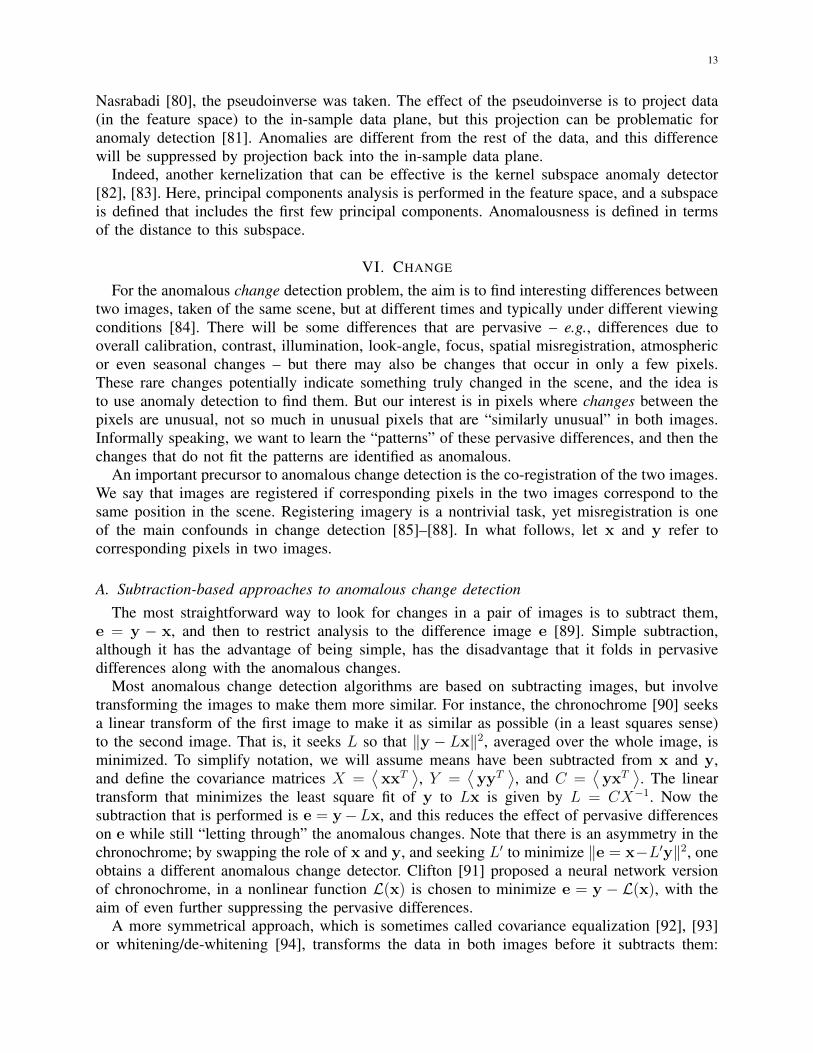
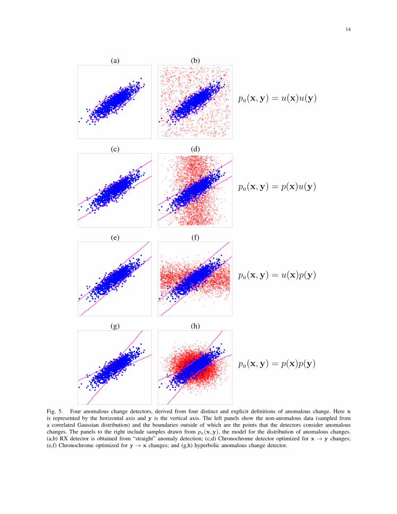
Fig. 5. Four anomalous change detectors, derived from four distinct and explicit definitions of anomalous change. Here xis represented by the horizontal axis and y is the vertical axis. The left panels show the non-anomalous data (sampled froma correlated Gaussian distribution) and the boundaries outside of which are the points that the detectors consider anomalouschanges. The panels to the right include samples drawn from pa(x,y), the model for the distribution of anomalous changes.(a,b) RX detector is obtained from “straight” anomaly detection; (c,d) Chronochrome detector optimized for x → y changes;(e,f) Chronochrome optimized for y→ x changes; and (g,h) hyperbolic anomalous change detector.

15

e = Y −1/2y−X−1/2x. It can be shown [95] that this is related to canonical coordinate analysisand to Nielsen’s multivariate alteration detection (MAD) algorithm [96] and to a “total leastsquares” change detection algorithm [97]. One reason there are so many variants is that thereis not a unique whitening transform: if U is an arbitrary orthogonal matrix, then UX−1/2 willalso whiten the x samples. That is: if x = UX−1/2x, then we say that x is whitened because⟨xxT

⟩= I .

In all of these algorithms, a vector-valued difference, e, is produced. For anomaly detection,we need a scalar valued measure of anomalousness, and the RX formula provides the moststraightforward way to achieve that. Let E =

⟨eeT

⟩be the covariance matrix of the residuals,

and then take the anomalousness to be

A(e) = eTE−1e (24)

As a particular example, we can write Eq. (24) for the chronochrome detector. Here e =y − CX−1x, and

A(x,y) = (y − CX−1x)T [Y − CX−1C]−1(y − CX−1x) (25)

B. Distribution-based approaches to anomalous change detectionWhile subtracting (suitably transformed) images is an intuitively plausible way to look for

anomalous changes, we can take more of a machine learning point of view and treat the problemas one of two-class classification, where the two classes are pervasive differences and anomalouschanges. If we can write down expressions for the underlying distributions of these two classes,then their ratio will be an optimal detector of anomalous changes.

The distribution for the pervasive differences is just the distribution of the data itself. Wecan call this pb(x,y) to indicate that it is the “background” distribution. What we need is agenerative model for anomalous changes; that is, a distribution pa(x,y) that describes what wemean when we speak of anomalous changes. What that in hand, our anomaly detector is givenby the likelihood ratio

L(x,y) = pa(x,y)

pb(x,y). (26)

The simplest choice, following our experience with straight anomaly detection, is a uniformdistribution. We can write this pa(x,y) = u(x)u(y). This is not an unreasonable choice, butit does not put any particular emphasis on change. A pair of pixels (x,y) that are “similarlyanomalous” in both images (e.g., the pixel might be unusually bright in both images) do notparticularly indicate that something has changed at that pixel position in the scene.

But there are alternative models pa(x,y) that correspond to different notions of what ananomalous change is. For instance, if we are thinking specifically of changes x→ y, where x isa kind of “reference” image, and y is the new image that might contain the changes of interest,then pa(x,y) = pb(x)u(y). This corresponds to a non-anomalous x and an anomalous y. It isinteresting to note that using this definition of anomaly in Eq. (26) leads to L(x,y) = 1/pb(y|x),so that anomalousness of y varies inversely with the conditional probability density of y. Aswith the chronochrome4, there is an asymmetry in this model of anomalous change; its mirrorimage is the situation in which y is considered the reference image and it is y → x changesthat are of particular interest; here, pa(x,y) = u(x)pb(y).

4In fact, the chronochrome can be obtained from this model in the special case that pb(x,y) is Gaussian [98].

16

Another choice for pa(x,y) has also been suggested [99]. Here, pa(x,y) = pb(x)pb(y), andx → y and y → x changes are treated equally. The informal interpretation is that unusualchanges are pixel pairs (x,y) which are collectively unusual, but individually normal. That is,the x pixel value is typical for the x-image, and the y pixel value is typical for the y-image, butthe (x,y) pair is unusual. If we use this model for anomalies in Eq. (26), and take a logarithm,we obtain

logL(x,y) = log pb(x) + log pb(y)− log pb(x,y) (27)

an expression for anomalousness that looks like negative mutual information of x and y.In the case of Gaussian pb(x,y), Eq. (27) reduces to a quadratic expression in x and y that has

hyperbolic contours (see Fig. 5(g,h)). Experiments with real and simulated anomalous changesin real imagery indicated that this hyperbolic anomalous change detection (HACD) generallyoutperformed the subtraction-based anomaly detectors [95].

A further advantage of the distribution-based approach is that the distribution needn’t be Gaus-sian. Indeed, we can take a purely nonparametric view, and treat the problem of distinguishingpervasive differences from anomalous changes as a machine learning classification. Steinwart etal. [100] used support vector machines for just this purpose. But a simpler approach, that has alsoproven effective, is to consider a parametric distribution, but one slightly more general than theGaussian. The class of elliptically-contoured (EC) distributions are, like the Gaussian, primarilyparameterized by a mean vector and covariance matrix, but do not share the sharp e−r

2 tailof the Gaussian. Heavy-tailed EC distributions have been suggested for hyperspectral imageryin general [101], and for anomalous change detection in particular [102], [103]. Although ECdistributions do not affect the “straight anomaly detector” shown in Fig. 5(a,b), they do generalizechronochrome and hyperbolic anomalous change detectors in a way that can lead to improvedperformance [103]. Kernelization of the EC-based change detector has also been shown to beadvantageous [104].

C. Further comments on anomalous change detectionThe description here treats pixel pairs as independent samples from an unknown distribution.

But there is a lot of spatial structure in imagery, and further gains can be made by incorporatingspatial aspects along with the spectral [105], [106]. The description here also considers onlypairs of images; often there are more than two images, and these algorithms can be extended tothat case [107], [108], though this approach may not be optimal for sequences of images (e.g.,anomalous activities in video) where the order of the images in the sequence matters. Anotherissue that arises in remote sensing is that the anomalous targets may be subpixel in extent, whichleads to a different optimization problem [109].

Anomalous change detection is a problem that is particularly well matched to remote sensingimagery, and in that context, a variety of practical issues have been discussed [110], [111]. Oneof the biggest of these issues is misregistration, when the images don’t exactly line up (and theynever exactly line up). Although the effects of misregistration can to some extent be learnedfrom the pervasive differences it creates in image pairs, it is still one of the main confoundsto change detection [85], [86]. Gains can be made by explicitly adapting the change detectionalgorithm to be more robust to misregistration error [87], [88].

VII. CONCLUSION

Anomaly detection is seldom a goal in its own right. It is the first step in a search for datasamples that are relevant, meaningful, or – in some sense that depends on where the data came

17

from and what they are being used for – interesting.The mystical “by definition undefined” aspect of anomaly detection mostly derives from

the ambiguity of what one means by “interesting” and this has led to a wide variety of adhoc anomaly detection algorithms, justified by hand-waving arguments and validated (if atall) by anecdotal performance on imagery with a statistically inadequate number of pre-judgedanomalies.

By employing a framework in which anomalies are in fact well-defined, as samples drawnfrom some broad and flat distribution, anomaly detection algorithms can be objectively tested,and improvements can be confidently constructed.

Within this framework, many of the tools that have been developed for signal processing,machine learning, and data analytics in general, can be brought to bear on the detection ofanomalies. These range from the venerable Gaussian distribution to kernels and subspaces (andkernelized subspaces!), and invoke the usual issues in underfitting and overfitting data.

The technical challenge of anomaly detection is not usually the anomalies themselves, but withcharacterizing what can be a complex and highly structured background. Since most anomalydetection scenarios require a low false alarm rate, it is out on the periphery of this backgroundwhere the modeling is emphasized. This is something of a challenge, since the data density ismuch lower there. The modeling, however is discriminative, not generative, which means thatthe aim is not the model the distribution per se, but to find the boundary that separates thenon-anomalous data from the anomalies.

REFERENCES

1. S. Matteoli, M. Diani, and G. Corsini, “A tutorial overview of anomaly detection in hyperspectral images.”IEEE A&E Systems Magazine 25, 5–27 (2010).

2. D. W. J. Stein, S. G. Beaven, L. E. Hoff, E. M. Winter, A. P. Schaum, and A. D. Stocker, “Anomaly detectionfrom hyperspectral imagery.” IEEE Signal Processing Magazine 19, 58–69 (Jan, 2002).

3. E. A. Ashton, “Multialgorithm solution for automated multispectral target detection.” Optical Engineering38, 717–724 (1999).

4. B. A. Whitehead and W. A. Hoyt, “Function approximation approach to anomaly detection in propulsionsystem test data.” J. Propulsion and Power 11, 1074–1076 (1995).

5. K. Worden, “Structural fault detection using a novelty measure.” J. Sound and Vibration 201, 85–101 (1997).6. C. Manikopoulos and S. Papavassiliou, “Network intrusion and fault detection: a statistical anomaly

approach.” IEEE Communications Magazine 40, no. 10, 76–82 (2002).7. M. Thottan and C. Ji, “Anomaly detection in IP networks.” IEEE Trans. Signal Processing 51, 2191–2204

(2003).8. D. M. Cai, M. Gokhale, and J. Theiler, “Comparison of feature selection and classification algorithms in

identifying malicious executables.” Computational Statistics and Data Analysis 51, 3156–3172 (2007).9. B. Scholkopf, R. C. Williamson, A. J. Smola, J. Shawe-Taylor, and J. C. Platt, “Support vector method for

novelty detection.” Advances in Neural Information Processing Systems 12, 582–588 (1999).10. M. Markou and S. Singh, “Novelty detection: a review – part 1: statistical approaches.” Signal Processing

83, 2481–2497 (2003).11. M. Markou and S. Singh, “Novelty detection: a review – part 2: neural network based approaches.” Signal

Processing 83, 2499–2521 (2003).12. D. M. Tax, One-class classification: Concept-learning in the absence of counter-examples. (TU Delft, Delft

University of Technology, 2001).13. L. M. Manevitz and M. Yousef, “One-class SVMs for document classification.” J. Machine Learning Res.

2, 139–154 (2001).14. J. Theiler, “By definition undefined: adventures in anomaly (and anomalous change) detection.” Proc. 6th

IEEE Workshop on Hyperspectral Signal and Image Processing: Evolution in Remote Sensing (WHISPERS)(2014).

18

15. I. Steinwart, D. Hush, and C. Scovel, “A classification framework for anomaly detection.” J. Machine LearningResearch 6, 211–232 (2005).

16. E. L. Lehmann and J. P. Romano, Testing Statistical Hypotheses. (Springer, New York, 2005).17. J. Theiler, “Confusion and clairvoyance: some remarks on the composite hypothesis testing problem.” Proc.

SPIE 8390, 839003 (2012).18. P. C. Mahalanobis, “On the generalised distance in statistics.” Proc. National Institute of Sciences of India

2, 49–55 (1936).19. I. S. Reed and X. Yu, “Adaptive multiple-band CFAR detection of an optical pattern with unknown spectral

distribution.” IEEE Trans. Acoustics, Speech, and Signal Processing 38, 1760–1770 (1990).20. A. D. Stocker, I. S. Reed, and X. Yu, “Multi-dimensional signal processing for electro-optical target detection.”

Proc. SPIE 1305, 218–231 (1990).21. A. Schaum, “Hyperspectral anomaly detection: Beyond RX.” Proc. SPIE 6565, 656502 (2007).22. J. Theiler and D. M. Cai, “Resampling approach for anomaly detection in multispectral images.” Proc. SPIE

5093, 230–240 (2003).23. A. Hayden, E. Niple, and B. Boyce, “Determination of trace-gas amounts in plumes by the use of orthogonal

digital filtering of thermal-emission spectra.” Applied Optics 35, 2802–2809 (1996).24. J. Theiler and B. Wohlberg, “Detection of unknown gas-phase chemical plumes in hyperspectral imagery.”

Proc. SPIE 8743, 874315 (2013).25. S. Matteoli, M. Diani, and J. Theiler, “An overview background modeling for detection of targets and

anomalies in hyperspectral remotely sensed imagery.” IEEE J. Sel. Topics in Applied Earth Observationsand Remote Sensing 7, 2317–2336 (2014).

26. Y. Cohen, Y. August, D. G. Blumberg, and S. R. Rotman, “Evaluating sub-pixel target detection algorithmsin hyper-spectral imagery.” J. Electrical and Computer Engineering 2012, 103286 (2012).

27. S. Matteoli, M. Diani, and G. Corsini, “Improved estimation of local background covariance matrix foranomaly detection in hyperspectral images.” Optical Engineering 49, 046201 (2010).

28. J. H. Friedman, “Regularized discriminant analysis.” J. Am. Statistical Assoc. 84, 165–175 (1989).29. N. M. Nasrabadi, “Regularization for spectral matched filter and RX anomaly detector.” Proc. SPIE 6966,

696604 (2008).30. J. P. Hoffbeck and D. A. Landgrebe, “Covariance matrix estimation and classification with limited training

data.” IEEE Trans. Pattern Analysis and Machine Intelligence 18, 763–767 (1996).31. J. Theiler, “The incredible shrinking covariance estimator.” Proc. SPIE 8391, 83910P (2012).32. G. Cao and C. A. Bouman, “Covariance estimation for high dimensional data vectors using the sparse matrix

transform.” Advances in Neural Information Processing Systems 21, 225–232 (2009).33. J. Theiler, G. Cao, L. R. Bachega, and C. A. Bouman, “Sparse matrix transform for hyperspectral image

processing.” IEEE J. Selected Topics in Signal Processing 5, 424–437 (2011).34. C. E. Caefer, J. Silverman, O. Orthal, D. Antonelli, Y. Sharoni, and S. R. Rotman, “Improved covariance

matrices for point target detection in hyperspectral data.” Optical Engineering 47, 076402 (2008).35. M. J. Carlotto, “A cluster-based approach for detecting man-made objects and changes in imagery.” IEEE

Trans. Geoscience and Remote Sensing 43, 374–387 (2005).36. J. Theiler and L. Prasad, “Overlapping image segmentation for context-dependent anomaly detection.” Proc.

SPIE 8048, 804807 (2011).37. P. J. Rousseeuw and A. M. Leroy, Robust Regression and Outlier Detection. (Wiley-Interscience, New York,

1987).38. S. Matteoli, M. Diani, and G. Corsini, “Hyperspectral anomaly detection with kurtosis-driven local covariance

matrix corruption mitigation.” IEEE Geoscience and Remote Sensing Lett. 8, 532–536 (2011).39. S. Matteoli, M. Diani, and G. Corsini, “Impact of signal contamination on the adaptive detection performance

of local hyperspectral anomalies.” IEEE Trans. Geoscience and Remote Sensing 52, 1948–1968 (2014).40. W. F. Basener, “Clutter and anomaly removal for enhanced target detection.” Proc. SPIE 7695, 769525 (2010).41. G. Grosklos and J. Theiler, “Ellipsoids for anomaly detection in remote sensing imagery.” Proc. SPIE 9472,

94720P (2015).42. J. Theiler and J. Bloch, “Multiple concentric annuli for characterizing spatially nonuniform backgrounds.”

The Astrophysical Journal 519, 372–388 (1999).43. C. E. Caefer, M. S. Stefanou, E. D. Nelson, A. P. Rizzuto, O. Raviv, and S. R. Rotman, “Analysis of false

alarm distributions in the development and evaluation of hyperspectral point target detection algorithms.”

19

Optical Engineering 46, 076402 (2007).44. J. Theiler, “Symmetrized regression for hyperspectral background estimation.” Proc. SPIE 9472, 94721G

(2015).45. N. Hasson, S. Asulin, S. R. Rotman, and D. Blumberg, “Evaluating backgrounds for subpixel target detection:

when closer isn’t better.” Proc. SPIE 9472, 94720R (2015).46. J. Theiler and B. Wohlberg, “Regression framework for background estimation in remote sensing imagery.”

Proc. 5th IEEE Workshop on Hyperspectral Image and Signal Processing: Evolution in Remote Sensing(WHISPERS) (2013).

47. W. F. Basener, E. Nance, and J. Kerekes, “The target implant method for predicting target difficulty anddetector performance in hyperspectral imagery.” Proc. SPIE 8048, 80481H (2011).

48. J. Theiler, “Matched-pair machine learning.” Technometrics 55, 536–547 (2013).49. D. Tax and R. Duin, “Uniform object generation for optimizing one-class classifiers.” J. Machine Learning

Res. 2, 155–173 (2002).50. T. Hastie, R. Tibshirani, and J. Friedman, Elements of Statistical Learning: Data Mining, Inference, and

Prediction. (Springer-Verlag, New York, 2001). This anomaly detection approach is developed in Chapter14.2.4, and illustrated in Fig 14.3.

51. J. Theiler and D. Hush, “Statistics for characterizing data on the periphery.” Proc. IEEE Int. Geoscience andRemote Sensing Symposium (IGARSS) 4764–4767 (2010).

52. J. Theiler, “Ellipsoid-simplex hybrid for hyperspectral anomaly detection.” Proc. 3rd IEEE Workshop onHyperspectral Image and Signal Processing: Evolution in Remote Sensing (WHISPERS) (2011).

53. L. Bachega, J. Theiler, and C. A. Bouman, “Evaluating and improving local hyperspectral anomaly detectors.”IEEE Applied Imagery and Pattern Recognition (AIPR) Workshop 39 (2011).

54. N. A. Campbell, “Robust procedures in multivariate analysis I: Robust covariance estimation.” AppliedStatistics 29, 231–237 (1980).

55. P. J. Rousseeuw and K. Van Driessen, “A fast algorithm for the minimum covariance determinant estimator.”Technometrics 41, 212–223 (1999).

56. L. G. Khachiyan, “Rounding of polytopes in the real number model of computation.” Mathematics ofOperations Research 21, 307–320 (1996).

57. P. Kumar and E. A. Yildirim, “Minimum-volume enclosing ellipsoids and core sets.” J. Optimization Theoryand Applications 126, 1–21 (2005).

58. M. J. Todd and E. A. Yildirim, “On Khachiyan’s algorithm for the computation of minimum-volume enclosingellipsoids.” Discrete Applied Mathematics 155, 1731–1744 (2007).

59. J. Theiler, B. R. Foy, and A. M. Fraser, “Characterizing non-Gaussian clutter and detecting weak gaseousplumes in hyperspectral imagery.” Proc. SPIE 5806, 182–193 (2005).

60. P. Bajorski, “Maximum Gaussianity models for hyperspectral images.” Proc. SPIE 6966, 69661M (2008).61. S. M. Adler-Golden, “Improved hyperspectral anomaly detection in heavy-tailed backgrounds.” Proc. 1st

IEEE Workshop on Hyperspectral Image and Signal Processing: Evolution in Remote Sensing (WHISPERS)(2009).

62. S. T. Roweis and L. K. Saul, “Nonlinear dimensionality reduction by locally linear embedding.” Science 290,2323–2326 (2000).

63. J. B. Tenenbaum, V. de Silva, and J. C. Langford, “A global geometric framework for nonlinear dimensionalityreduction.” Science 290, 2319–2323 (2000).

64. C. M. Bachmann, T. L. Ainsworth, and R. A. Fusina, “Exploiting manifold geometry in hyperspectralimagery.” IEEE Trans. Geoscience and Remote Sensing 43, 441–454 (2005).

65. D. Lunga, S. Prasad, M. M. Crawford, and O. Ersoy, “Manifold-learning-based feature extraction forclassification of hyperspectral data: A review of advances in manifold learning.” IEEE Signal ProcessingMagazine 31, 55–66 (Jan, 2014).

66. A. K. Ziemann and D. W. Messinger, “An adaptive locally linear embedding manifold learning approach forhyperspectral target detection.” Proc. SPIE 9472, 94720O (2015).

67. K. Ranney and M. Soumekh, “Hyperspectral anomaly detection within the signal subspace.” IEEE Geoscienceand Remote Sensing Letters 3, 312–316 (2006).

68. L. Ma, M. M. Crawford, and J. Tian, “Anomaly detection for hyperspectral images based on robust locallylinear embedding.” J. Infrared Millimeter Terahertz Waves 31, 753–762 (2010).

69. G. A. Tidhar and S. R. Rotman, “Target detection in inhomogeneous non-Gaussian hyperspectral data based

20

on nonparametric density estimation.” Proc. SPIE 8743, 87431A (2013).70. H. Kwon, S. Z. Der, and N. M. Nasrabadi, “Adaptive anomaly detection using subspace separation for

hyperspectral imagery.” Optical Engineering 42, 3342–335171. E. Parzen, “On estimation of probability density function and mode.” Ann. Mathematical Statistics 33, 1065–

1076 (1962).72. S. Matteoli, T. Veracini, M. Diani, and G. Corsini, “Background density nonparametric estimation with data-

adaptive bandwidths for the detection of anomalies in multi-hyperspectral imagery.” IEEE Geoscience andRemote Sensing Lett. 11, 163–167 (2014).

73. S. Matteoli, T. Veracini, M. Diani, and G. Corsini, “A locally adaptive background density estimator: Anevolution for RX-based anomaly detectors.” IEEE Geoscience and Remote Sensing Lett. 11, 323–327 (2014).

74. B. Basener, E. Ientilucci, and D. Messinger, “Anomaly detection using topology.” Proc. SPIE 6565, 65650J(2007).

75. W. F. Basener and D. W. Messinger, “Enhanced detection and visualization of anomalies in spectral imagery.”Proc. SPIE 7334, 73341Q (2009).

76. C. Scovel, D. Hush, I. Steinwart, and J. Theiler, “Radial kernels and their reproducing kernel Hilbert spaces.”J. Complexity 26, 641–660 (2010).

77. D. Tax and R. Duin, “Data domain description by support vectors.” In Proc. ESANN99, M. Verleysen, ed.(D. Facto Press, Brussels, 1999), pp. 251–256.

78. A. Banerjee, P. Burlina, and C. Diehl, “A support vector method for anomaly detection in hyperspectralimagery.” IEEE Trans. Geoscience and Remote Sensing 44, 2282–2291 (2006).

79. D. Cremers, T. Kohlberger, and C. Schnorr, “Shape statistics in kernel space for variational imagesegmentation.” Pattern Recognition 36, 1929–1943 (2003).

80. H. Kwon and N. Nasrabadi, “Kernel RX-algorithm: A nonlinear anomaly detector for hyperspectral imagery.”IEEE Trans. Geoscience and Remote Sensing 43, 388–397 (2005).

81. J. Theiler and G. Grosklos, “Problematic projection to the in-sample subspace for a kernelized anomalydetector.” IEEE Geoscience and Remote Sensing Lett. (2016). To appear.

82. H. Hoffmann, “Kernel PCA for novelty detection.” Pattern Recognition 40, 863–874 (2007).83. N. M. Nasrabadi, “Kernel subspace-based anomaly detection for hyperspectral imagery.” Proc. 1st IEEE

Workshop on Hyperspectral Signal and Image Processing: Evolution in Remote Sensing (WHISPERS) (2009).84. A. Schaum and E. Allman, “Advanced algorithms for autonomous hyperspectral change detection.” IEEE

Applied Imagery Pattern Recognition (AIPR) Workshop 33, 33–38 (2005).85. J. Theiler, “Sensitivity of anomalous change detection to small misregistration errors.” Proc. SPIE 6966,

69660X (2008).86. J. Meola and M. T. Eismann, “Image misregistration effects on hyperspectral change detection.” Proc. SPIE

6966, 69660Y (2008).87. J. Theiler and B. Wohlberg, “Local co-registration adjustment for anomalous change detection.” IEEE Trans.

Geoscience and Remote Sensing 50, 3107–3116 (2012).88. K. Vongsy, M. T. Eismann, and M. J. Mendenhall, “Extension of the linear chromodynamics model for

spectral change detection in the presence of residual spatial misregistration.” IEEE Trans. Geoscience andRemote Sensing 53, 3005–3021 (2015).

89. L. Bruzzone and D. F. Prieto, “Automatic analysis of the difference image for unsupervised change detection.”IEEE Trans. Geoscience and Remote Sensing 38, 1171–1182 (2000).

90. A. Schaum and A. Stocker, “Long-interval chronochrome target detection.” Proc. ISSSR (Int. Symposium onSpectral Sensing Research) (1998).

91. C. Clifton, “Change detection in overhead imagery using neural networks.” Applied Intelligence 18, 215–234(2003).

92. A. Schaum and A. Stocker, “Linear chromodynamics models for hyperspectral target detection.” Proc. IEEEAerospace Conference 1879–1885 (2003).

93. A. Schaum and A. Stocker, “Hyperspectral change detection and supervised matched filtering based oncovariance equalization.” Proc. SPIE 5425, 77–90 (2004).

94. R. Mayer, F. Bucholtz, and D. Scribner, “Object detection by using “whitening/dewhitening” to transformtarget signatures in multitemporal hyperspectral and multispectral imagery.” IEEE Trans. Geoscience andRemote Sensing 41, 1136–1142 (2003).

95. J. Theiler, “Quantitative comparison of quadratic covariance-based anomalous change detectors.” Applied

21

Optics 47, F12–F26 (2008).96. A. A. Nielsen, K. Conradsen, and J. J. Simpson, “Multivariate alteration detection (MAD) and MAF post-

processing in multispectral bi-temporal image data: new approaches to change detection studies.” RemoteSensing of the Environment 64, 1–19 (1998).

97. J. Theiler and A. Matsekh, “Total least squares for anomalous change detection.” Proc. SPIE 7695, 76951H(2010).

98. J. Theiler and S. Perkins, “Resampling approach for anomalous change detection.” Proc. SPIE 6565, 65651U(2007).

99. J. Theiler and S. Perkins, “Proposed framework for anomalous change detection.” ICML Workshop onMachine Learning Algorithms for Surveillance and Event Detection 7–14 (2006).

100. I. Steinwart, J. Theiler, and D. Llamocca, “Using support vector machines for anomalous change detection.”Proc. IEEE Int. Geoscience and Remote Sensing Symposium (IGARSS) 3732–3735 (2010).

101. D. Manolakis, D. Marden, J. Kerekes, and G. Shaw, “On the statistics of hyperspectral imaging data.” Proc.SPIE 4381, 308–316 (2001).

102. A. Schaum, E. Allman, J. Kershenstein, and D. Alexa, “Hyperspectral change detection in high clutter usingelliptically contoured distributions.” Proc. SPIE 6565, 656515 (2007).

103. J. Theiler, C. Scovel, B. Wohlberg, and B. R. Foy, “Elliptically-contoured distributions for anomalous changedetection in hyperspectral imagery.” IEEE Geoscience and Remote Sensing Lett. 7, 271–275 (2010).

104. N. Longbotham and G. Camps-Valls, “A family of kernel anomaly change detectors.” Proc. 6th IEEEWorkshop on Hyperspectral Signal and Image Processing: Evolution in Remote Sensing (WHISPERS) (2014).

105. T. Kasetkasem and P. K. Varshney, “An image change detection algorithm based on Markov random fieldmodels.” IEEE Trans. Geoscience and Remote Sensing 40, 1815–1823 (2002).

106. J. Theiler, “Spatio-spectral anomalous change detection in hyperspectral imagery.” Proc. 1st IEEE GlobalSignal and Information Processing Conference 953–956 (2013).

107. S. M. Adler-Golden, S. C. Richtsmeier, and R. Shroll, “Suppression of subpixel sensor jitter fluctuationsusing temporal whitening.” Proc. SPIE 6969, 69691D (2008).

108. J. Theiler and S. M. Adler-Golden, “Detection of ephemeral changes in sequences of images.” IEEE AppliedImagery Pattern Recognition (AIPR) Workshop 37 (2009).

109. J. Theiler, “Subpixel anomalous change detection in remote sensing imagery.” Proc. IEEE SouthwestSymposium on Image Analysis and Interpretation 165–168 (2008).

110. M. T. Eismann, J. Meola, and R. Hardie, “Hyperspectral change detection in the presence of diurnal andseasonal variations.” IEEE Trans. Geoscience and Remote Sensing 46, 237–249 (2008).

111. M. T. Eismann, J. Meola, A. D. Stocker, S. G. Beaven, and A. P. Schaum, “Airborne hyperspectral detectionof small changes.” Applied Optics 47, F27–F45 (2008).