1

An Asymptotically Optimal Algorithm for the Max k-Armed Bandit

Problem

Matthew Streeter & Stephen SmithCarnegie Mellon

UniversityNESCAI, April 29 2006

2

Outline Problem statement & motivations Modeling payoff distributions An asymptotically optimal algorithm

3

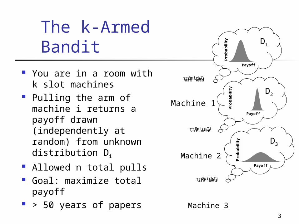
You are in a room with k slot machines

Pulling the arm of machine i returns a payoff drawn (independently at random) from unknown distribution Di

Allowed n total pulls Goal: maximize total payoff

> 50 years of papers

PayoffProbability

QuickTime™ and aTIFF (Uncompressed) decompressorare needed to see this picture.

Machine 1

D1

QuickTime™ and aTIFF (Uncompressed) decompressorare needed to see this picture.

PayoffProbability

Machine 2

D2

QuickTime™ and aTIFF (Uncompressed) decompressorare needed to see this picture.

PayoffProbability

Machine 3

D3

The k-Armed Bandit

4

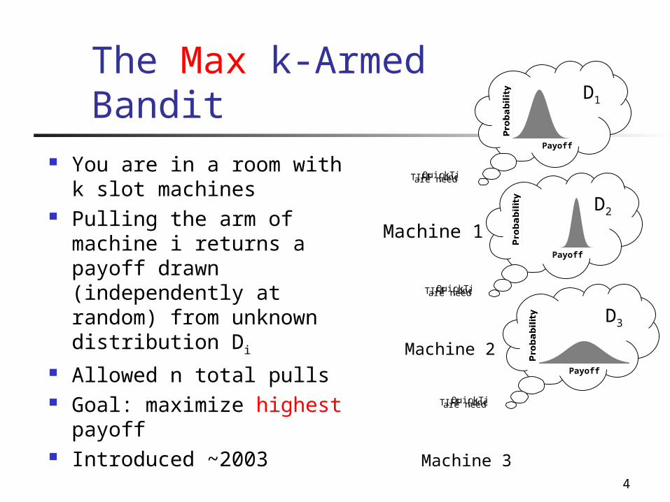
The Max k-Armed Bandit

You are in a room with k slot machines

Pulling the arm of machine i returns a payoff drawn (independently at random) from unknown distribution Di

Allowed n total pulls Goal: maximize highest payoff

Introduced ~2003

PayoffProbability

QuickTime™ and aTIFF (Uncompressed) decompressorare needed to see this picture.

Machine 1

D1

QuickTime™ and aTIFF (Uncompressed) decompressorare needed to see this picture.

PayoffProbability

Machine 2

D2

QuickTime™ and aTIFF (Uncompressed) decompressorare needed to see this picture.

PayoffProbability

Machine 3

D3

5

PayoffProbability

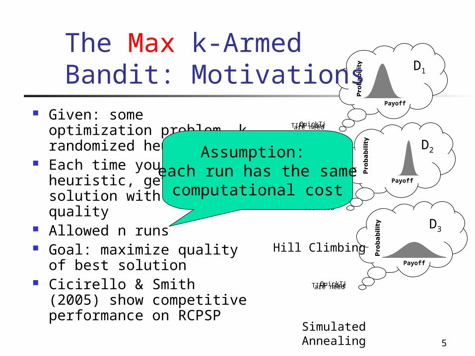
The Max k-Armed Bandit: Motivations

Given: some optimization problem, k randomized heuristics

Each time you run a heuristic, get a solution with a certain quality

Allowed n runs Goal: maximize quality of best solution

Cicirello & Smith (2005) show competitive performance on RCPSP

QuickTime™ and aTIFF (Uncompressed) decompressorare needed to see this picture.

QuickTime™ and aTIFF (Uncompressed) decompressorare needed to see this picture.

QuickTime™ and aTIFF (Uncompressed) decompressorare needed to see this picture.

PayoffProbability

PayoffProbability

Simulated Annealing

Hill Climbing

Tabu Search

D1

D2

D3

Assumption: each run has the samecomputational cost

6

The Max k-Armed Bandit: Example

Given n pulls, what strategy maximizes the (expected) maximum payoff? If n=1, should pull arm 1 (higher mean) If n=1000, should pull arm 2 (higher variance)

QuickTime™ and aTIFF (LZW) decompressor

are needed to see this picture.

7

Modeling Payoff Distributions

8

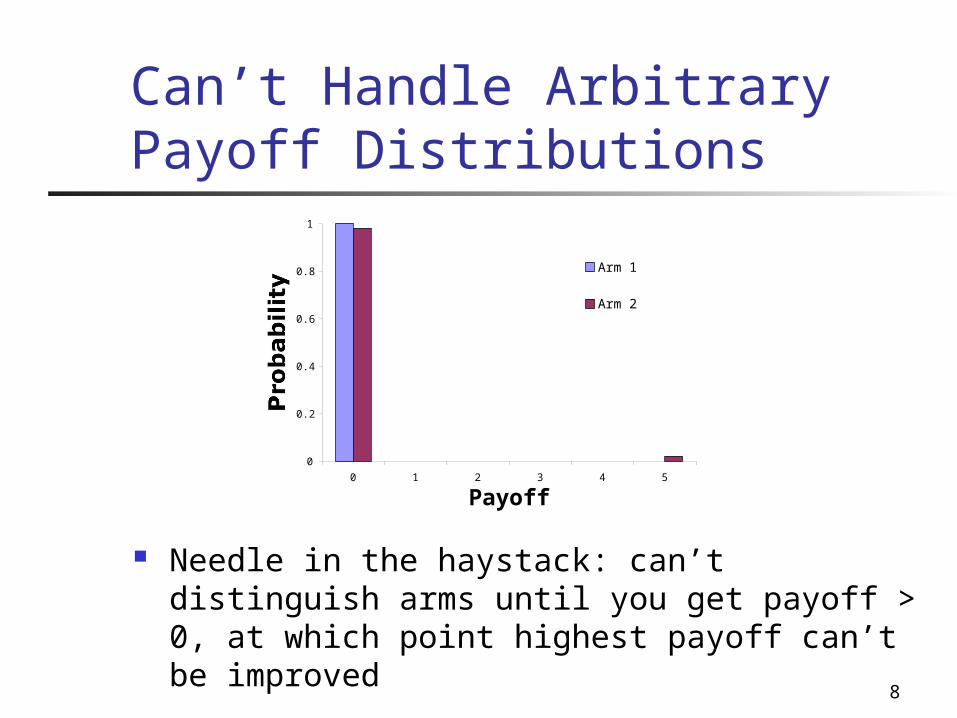
Can’t Handle Arbitrary Payoff Distributions

Needle in the haystack: can’t distinguish arms until you get payoff > 0, at which point highest payoff can’t be improved

0

0.2

0.4

0.6

0.8

1

0 1 2 3 4 5

Payoff

Probability

Arm 1

Arm 2

9

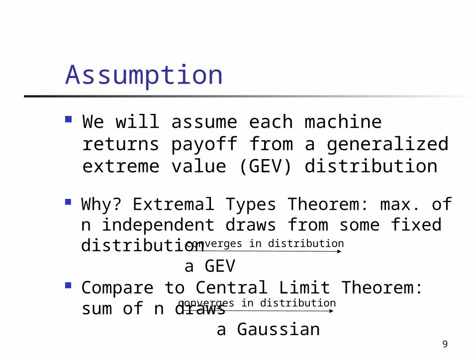
Assumption

We will assume each machine returns payoff from a generalized extreme value (GEV) distribution

Compare to Central Limit Theorem: sum of n draws a Gaussian

converges in distribution

converges in distribution

Why? Extremal Types Theorem: max. of n independent draws from some fixed distribution a GEV

10

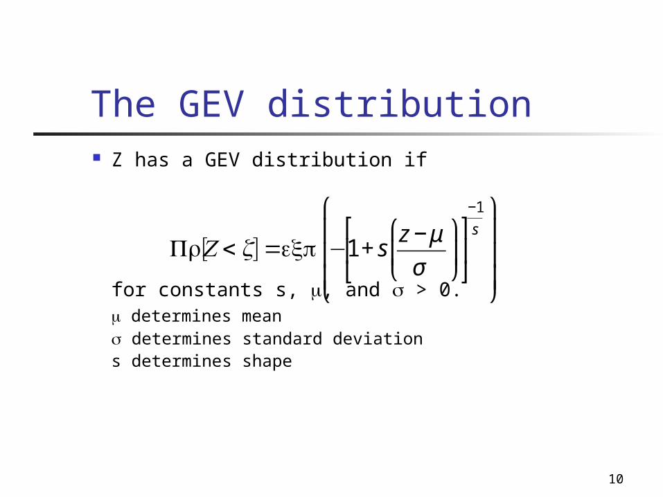
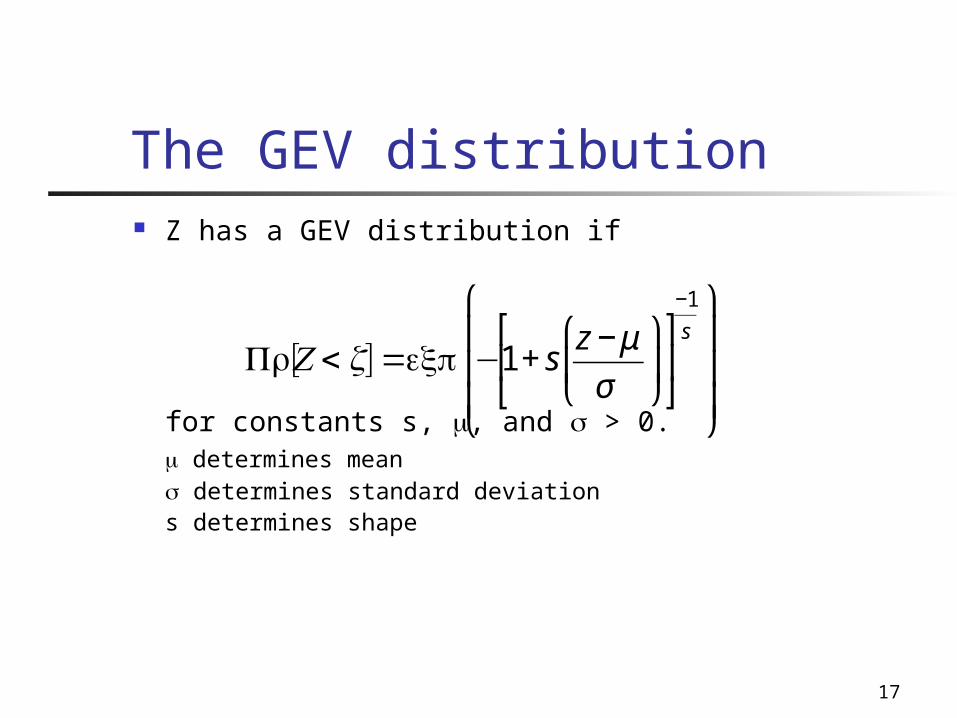
The GEV distribution Z has a GEV distribution if

for constants s, , and > 0. determines mean determines standard deviations determines shape

€

[Pr Z < z] =exp−1+ sz −μ

σ

⎛

⎝ ⎜

⎞

⎠ ⎟

⎡

⎣ ⎢

⎤

⎦ ⎥

−1

s ⎛

⎝

⎜ ⎜ ⎜

⎞

⎠

⎟ ⎟ ⎟

11

Example payoff distribution: Job Shop Scheduling Job shop scheduling: assign start times to operations, subject to constraints.

Length of schedule = latest completion time of any operation

Goal: find a schedule with minimum length

Many heuristics (branch and bound, simulated annealing...)

12

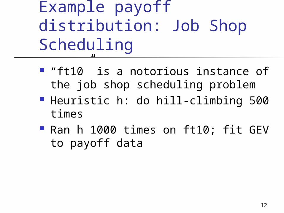
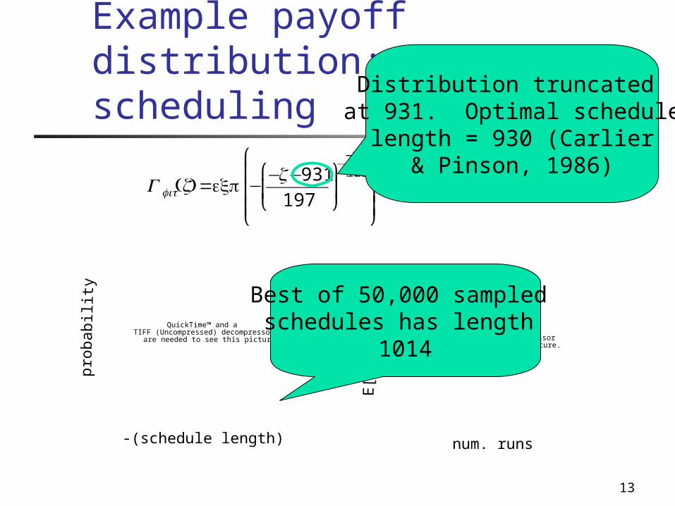
Example payoff distribution: Job Shop Scheduling “ft10” is a notorious instance of the job shop scheduling problem

Heuristic h: do hill-climbing 500 times

Ran h 1000 times on ft10; fit GEV to payoff data

13

Example payoff distribution: Job shop scheduling

€

Gfit(z)=exp−−z−931

197

⎛

⎝ ⎜

⎞

⎠ ⎟

−1

−.123 ⎛

⎝

⎜ ⎜ ⎜

⎞

⎠

⎟ ⎟ ⎟

QuickTime™ and aTIFF (Uncompressed) decompressor

are needed to see this picture.

-(schedule length)

prob

abili

ty

num. runs

QuickTime™ and aTIFF (Uncompressed) decompressor

are needed to see this picture.

E[M

ax. p

ayof

f]Best of 50,000 sampled schedules has length

1014

Distribution truncated at 931. Optimal schedulelength = 930 (Carlier

& Pinson, 1986)

14

An Asymptotically Optimal Algorithm

15

Notation

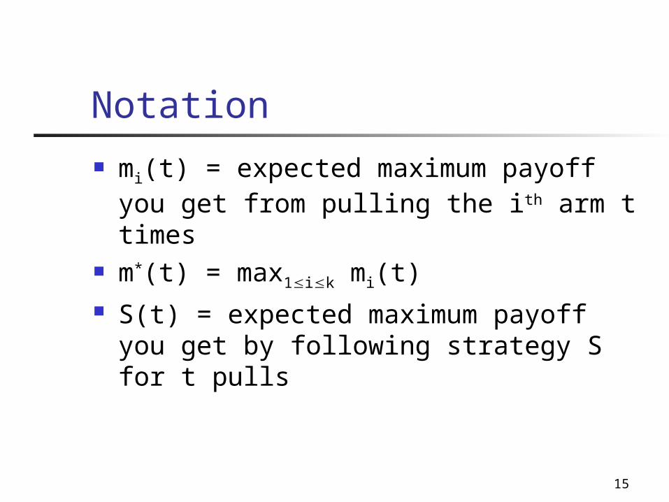
mi(t) = expected maximum payoff you get from pulling the ith arm t times

m*(t) = max1ik mi(t) S(t) = expected maximum payoff you get by following strategy S for t pulls

16

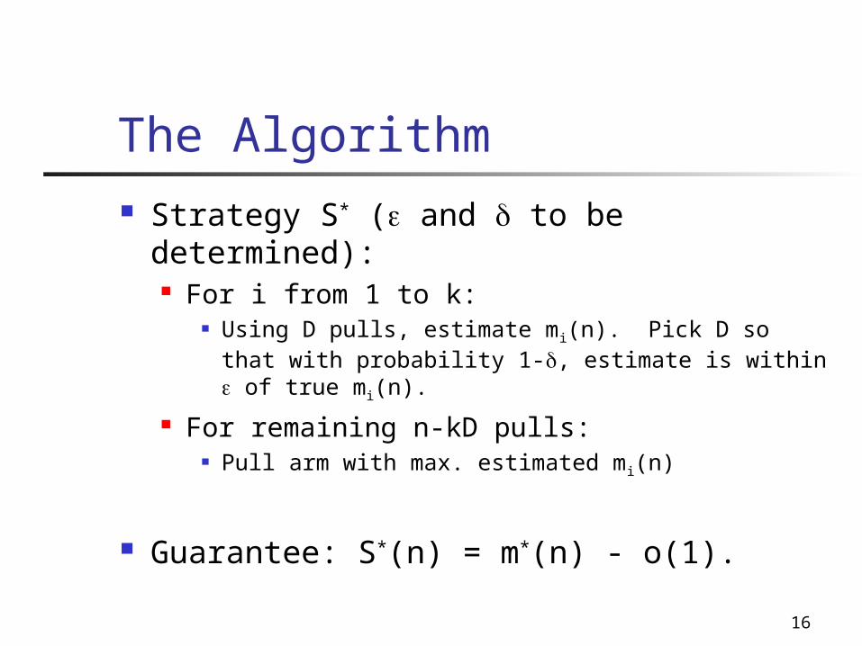
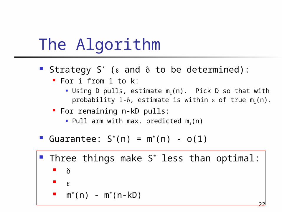
The Algorithm Strategy S* ( and to be determined): For i from 1 to k:

Using D pulls, estimate mi(n). Pick D so that with probability 1-, estimate is within of true mi(n).

For remaining n-kD pulls: Pull arm with max. estimated mi(n)

Guarantee: S*(n) = m*(n) - o(1).

17

The GEV distribution Z has a GEV distribution if

for constants s, , and > 0. determines mean determines standard deviations determines shape

€

[Pr Z < z] =exp−1+ sz −μ

σ

⎛

⎝ ⎜

⎞

⎠ ⎟

⎡

⎣ ⎢

⎤

⎦ ⎥

−1

s ⎛

⎝

⎜ ⎜ ⎜

⎞

⎠

⎟ ⎟ ⎟

18

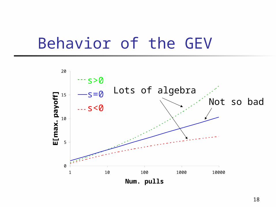
Behavior of the GEV

0

5

10

15

20

1 10 100 1000 10000

Num. pulls

E[max. payoff]

s=0

s<0

s>0Lots of algebra

Not so bad

19

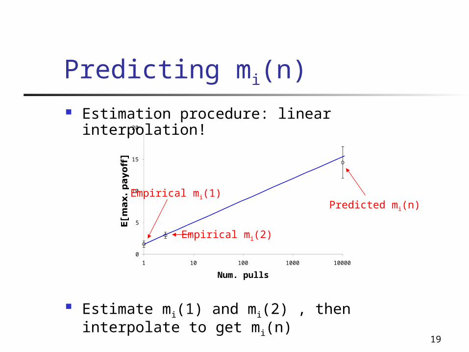
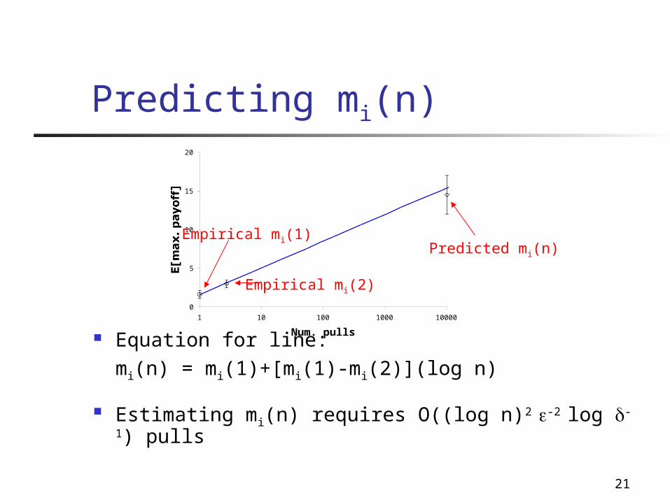
Estimation procedure: linear interpolation!

Estimate mi(1) and mi(2) , then interpolate to get mi(n)

Predicting mi(n)

0

5

10

15

20

1 10 100 1000 10000

Num. pulls

E[max. payoff]

Empirical mi(1)

Empirical mi(2)

Predicted mi(n)

20

Predicting mi(n): Lemma

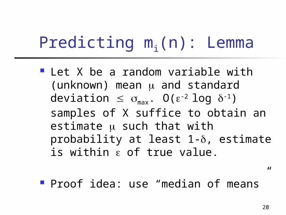
Let X be a random variable with (unknown) mean and standard deviation max. O(-2 log -1) samples of X suffice to obtain an estimate such that with probability at least 1-, estimate is within of true value.

Proof idea: use “median of means”

21

Equation for line: mi(n) = mi(1)+[mi(1)-mi(2)](log n)

Estimating mi(n) requires O((log n)2 -2 log -1) pulls

Predicting mi(n)

0

5

10

15

20

1 10 100 1000 10000

Num. pulls

E[max. payoff]

Empirical mi(1)

Empirical mi(2)

Predicted mi(n)

22

The Algorithm Strategy S* ( and to be determined):

For i from 1 to k: Using D pulls, estimate mi(n). Pick D so that with probability 1-, estimate is within of true mi(n).

For remaining n-kD pulls: Pull arm with max. predicted mi(n)

Guarantee: S*(n) = m*(n) - o(1)

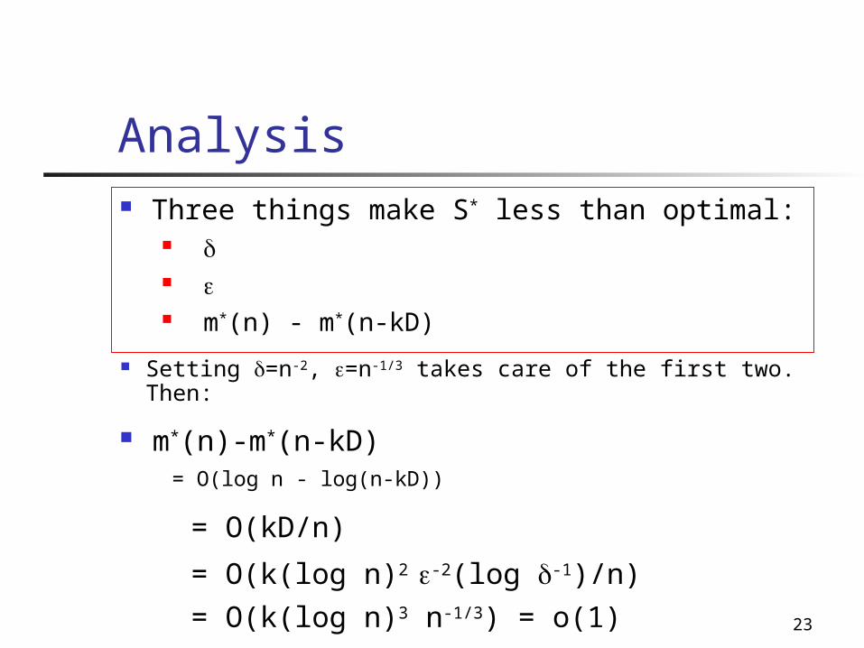
Three things make S* less than optimal: m*(n) - m*(n-kD)

23

Analysis

Setting =n-2, =n-1/3 takes care of the first two. Then:

m*(n)-m*(n-kD) = O(log n - log(n-kD))

= O(kD/n)

= O(k(log n)2 -2(log -1)/n) = O(k(log n)3 n-1/3) = o(1)

Three things make S* less than optimal: m*(n) - m*(n-kD)

24

Summary & Future Work Defined max k-armed bandit problem and discussed applications to heuristic search

Presented an asymptotically optimal algorithm for GEV payoff distributions (we analyzed special case s=0)

Working on applications to scheduling problems

25

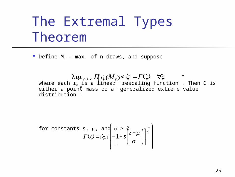
The Extremal Types Theorem Define Mn = max. of n draws, and suppose

where each rn is a linear “rescaling function”. Then G is either a point mass or a “generalized extreme value distribution”:

for constants s, , and > 0.

€

limn→∞ P rn Mn( ) < z[ ] =G(z) ∀z

€

G(z)=exp−1+ sz −μ

σ

⎛

⎝ ⎜

⎞

⎠ ⎟

⎡

⎣ ⎢

⎤

⎦ ⎥

−1

s ⎛

⎝

⎜ ⎜ ⎜

⎞

⎠

⎟ ⎟ ⎟