Embed Size (px)
Citation preview
1
Amit Fisher
Segev Wasserkrug
Dr. Opher Etzion
2
Outline
Motivation Introduction to Web Services Introduction to CLV RFM Variables Customer Relationship as Markov Chains Experimental Simulation Future Work
3
Motivation
Many Suppliers with similar offerings in E-Markets.
Customer will choose the organization that gives the better service
It is impossible to give the best service for all of customers all of the time (limited resources).
QoS refer to Response Time (RT) and availability
4
Solution in the Conventional Market
CRM (Customers Relationship Management): is a comprehensive approach which provides seamless integration of every area of business that touches the customer - namely marketing, sales, customer service and field support - through the integration of people, process and technology.
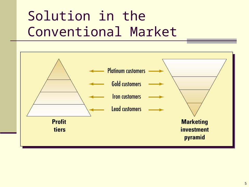
Implement techniques to give preference to valuable customers
5
Solution in the Conventional Market

6
Introduction to Web ServicesArchitectural EvolutionArchitectural Evolution Thin Clients interact
with a Main Frame
IBM
Main Frame
7
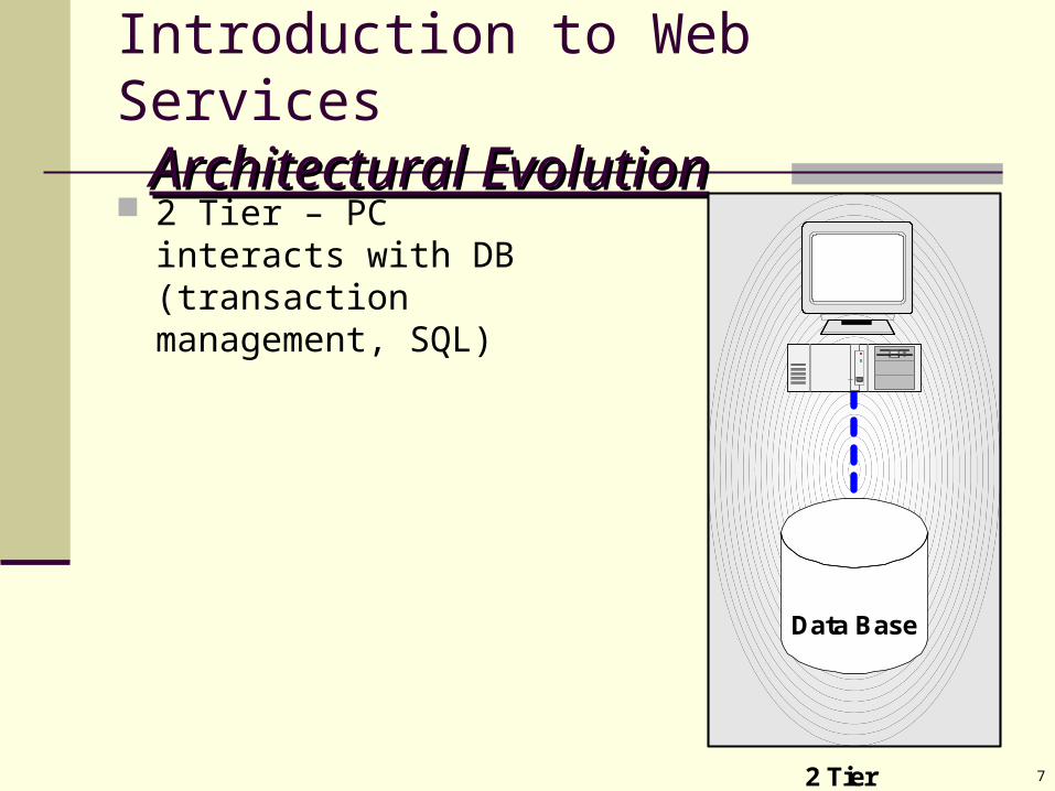
Introduction to Web Services Architectural EvolutionArchitectural Evolution 2 Tier – PC interacts
with DB (transaction management, SQL)
Data Base
2 Tier
8
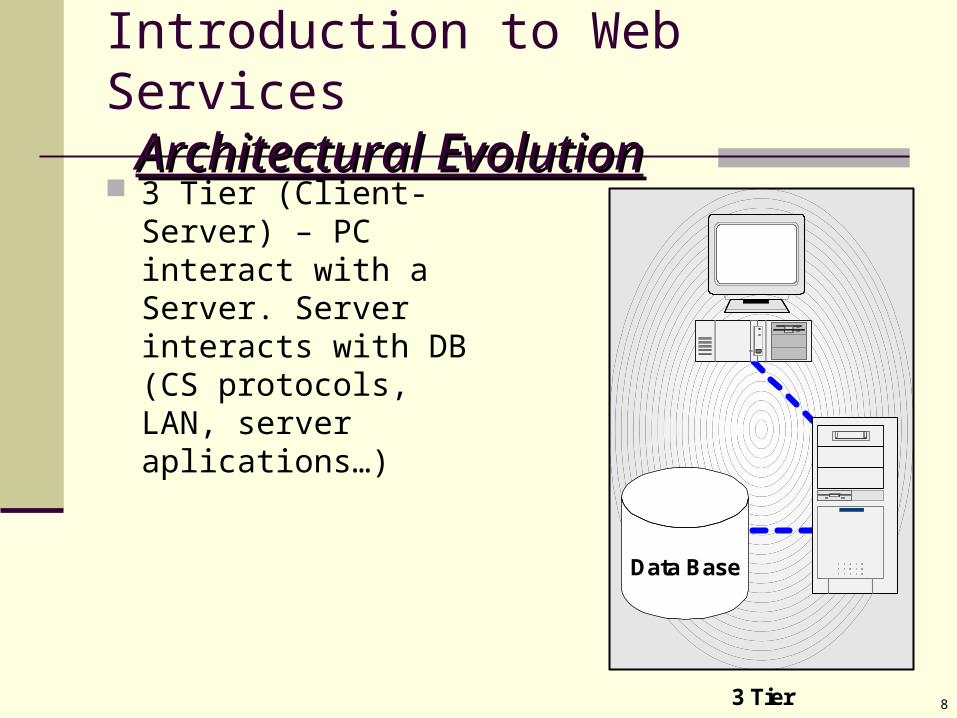
Introduction to Web Services Architectural EvolutionArchitectural Evolution 3 Tier (Client-Server) –
PC interact with a Server. Server interacts with DB (CS protocols, LAN, server aplications…)
Data Base
3 Tier
9
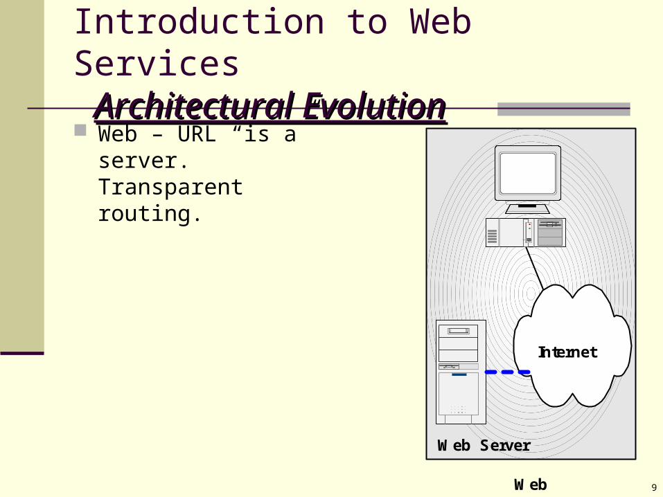
Introduction to Web Services Architectural EvolutionArchitectural Evolution Web – URL “is a”
server. Transparent routing.
Web Server
Web
Internet
10
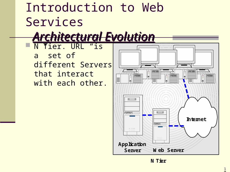
Introduction to Web Services Architectural EvolutionArchitectural Evolution N Tier. URL “is a” set
of different Servers that interact with each other.
Web Server
N Tier
Internet
ApplicationServer

11
Introduction to Web Services Architectural EvolutionArchitectural Evolution Web Services
Web Server
Internet
ApplicationServer
ApplicationServer
Web Server
12
Introduction to Web Services
A Web Service is a URL-addressable software resource that performs functions (or a function).
Web Services communicate using standard protocol known as SOAP (Simple Object Access Protocol).
A Web Service is located by its listing in a Universal Discovery, Description and Integration (UDDI) directory.
13
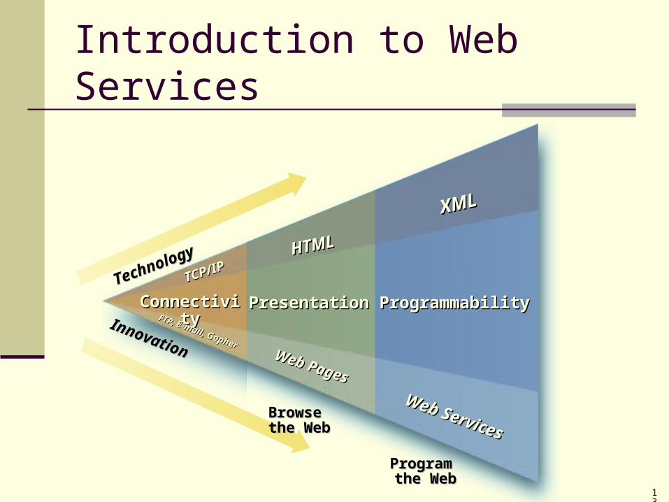
Introduction to Web Services
XMLXML
ProgrammabilityProgrammabilityConnectivityConnectivity
HTMLHTML
PresentationPresentation
TCP/IPTCP/IP
Technology
Technology
Innovation
Innovation
FTP,FTP, E-mail, Gopher
E-mail, GopherWeb Pages
Web Pages
Browse Browse the Webthe Web
Program Program the Webthe Web
Web Services
Web Services
14
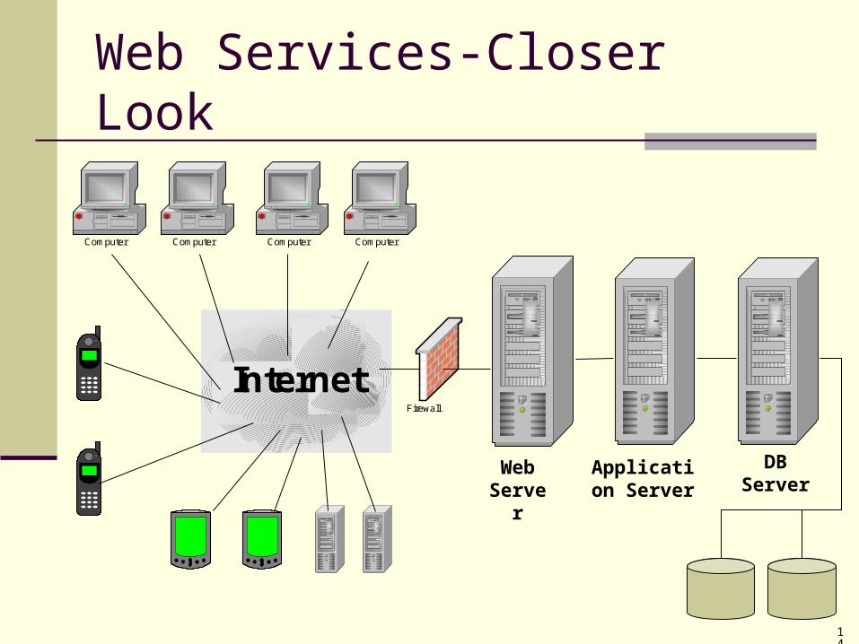
Web Services-Closer Look
Web Server
Application Server
DB Server
ComputerComputer Computer Computer
InternetFirewall
15
C
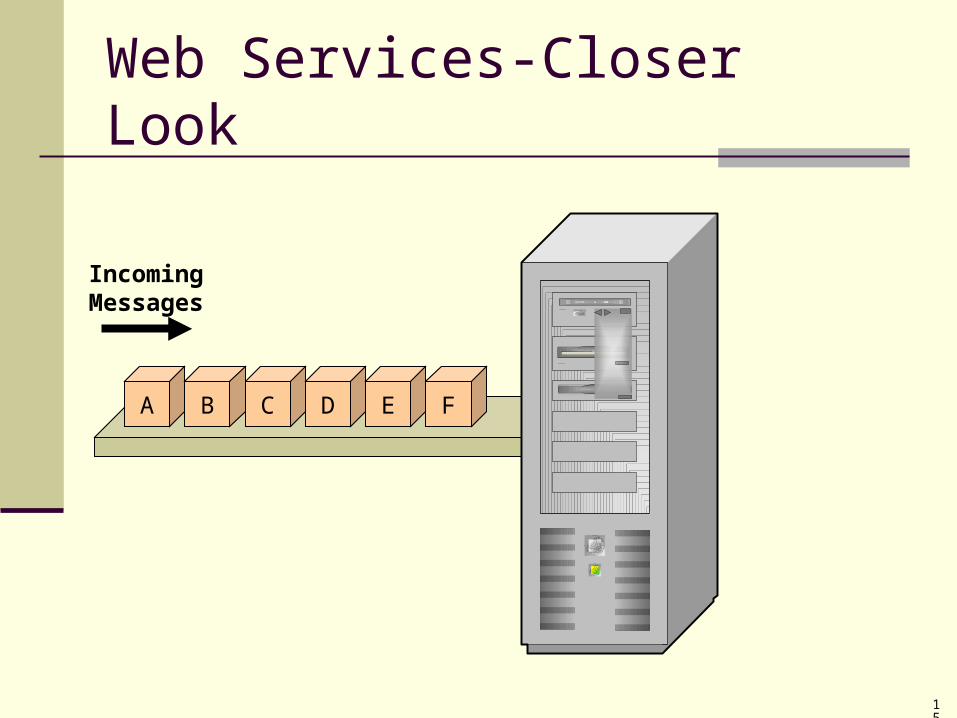
Web Services-Closer Look
A B
Incoming Messages
FD E
16
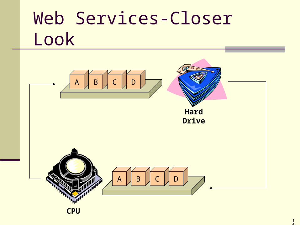
Web Services-Closer Look
CA B D
CA B D
Hard Drive
CPU
17
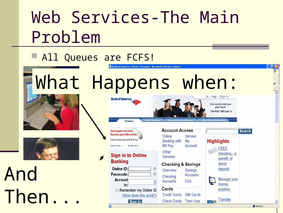
Web Services-The Main Problem
All Queues are FCFS!
What Happens when:
And Then...
18
Web Services-Our Solution
Preferred Customers must be served first. Who is preferred customer? CLV can differentiate between customers.
19
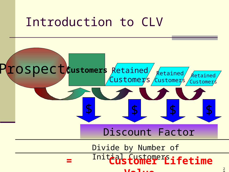
Introduction to CLV
CLV-projection of future cash flows for a customer across all product holdings and discounting these to get an "embedded value" of the customer.
20
Introduction to CLV
Prospects Customers
$ $ $ $
Discount Factor
Divide by Number of Initial Customers
= Customer Lifetime Value
RetainedCustomers
RetainedCustomers
RetainedCustomers
21
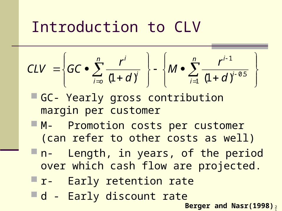
GC- Yearly gross contribution margin per customer
M- Promotion costs per customer (can refer to other costs as well)
n- Length, in years, of the period over which cash flow are projected.
r- Early retention rate d - Early discount rate
Introduction to CLV
n
ii
in
oii
i
d
rM
d
rGCCLV
15.0
1
)1()1(
Berger and Nasr(1998)
22
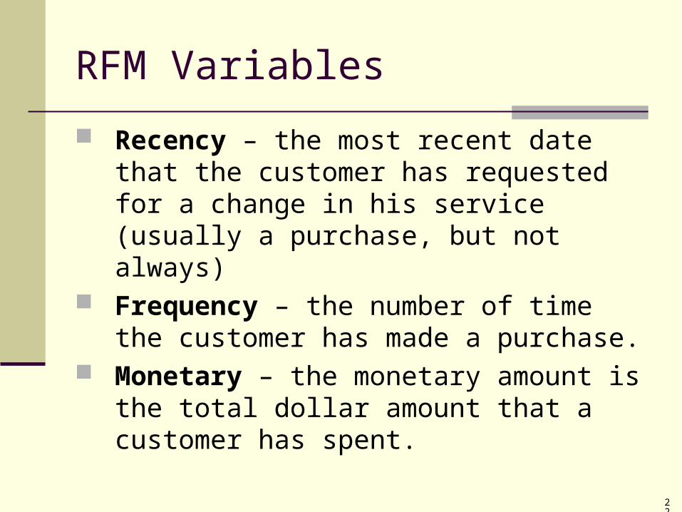
RFM Variables
Recency – the most recent date that the customer has requested for a change in his service (usually a purchase, but not always)
Frequency – the number of time the customer has made a purchase.
Monetary – the monetary amount is the total dollar amount that a customer has spent.
23
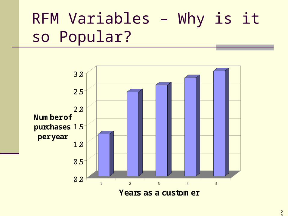
RFM Variables – Why is it so Popular?
0.0
0.5
1.0
1.5
2.0
2.5
3.0
Number of purchases per year
1 2 3 4 5
Years as a customer
24
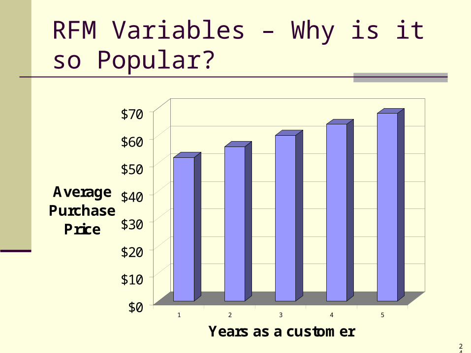
$0
$10
$20
$30
$40
$50
$60
$70
Average Purchase
Price
1 2 3 4 5
Years as a customer
RFM Variables – Why is it so Popular?
25
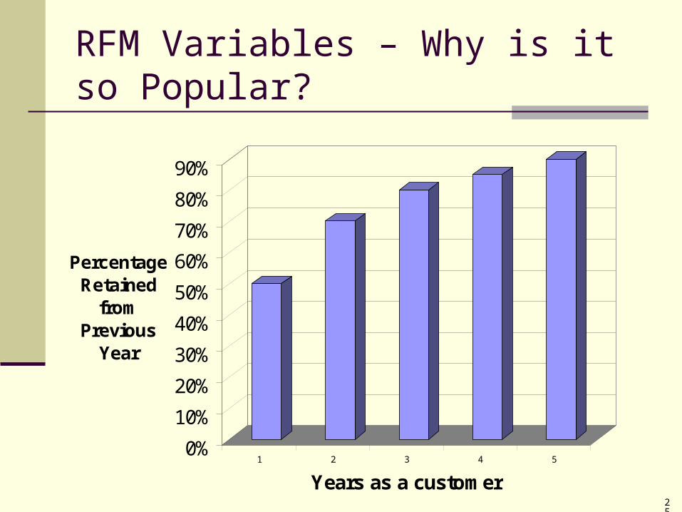
RFM Variables – Why is it so Popular?
0%
10%
20%
30%
40%
50%
60%
70%
80%
90%
Percentage Retained
from Previous
Year
1 2 3 4 5
Years as a customer
26
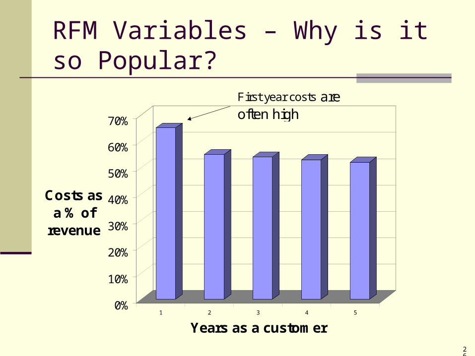
RFM Variables – Why is it so Popular?
0%
10%
20%
30%
40%
50%
60%
70%
Costs as a % of
revenue
1 2 3 4 5
Years as a customer
First year costs are often high
27
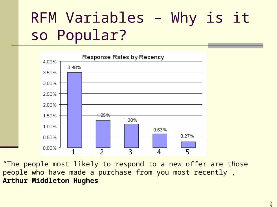
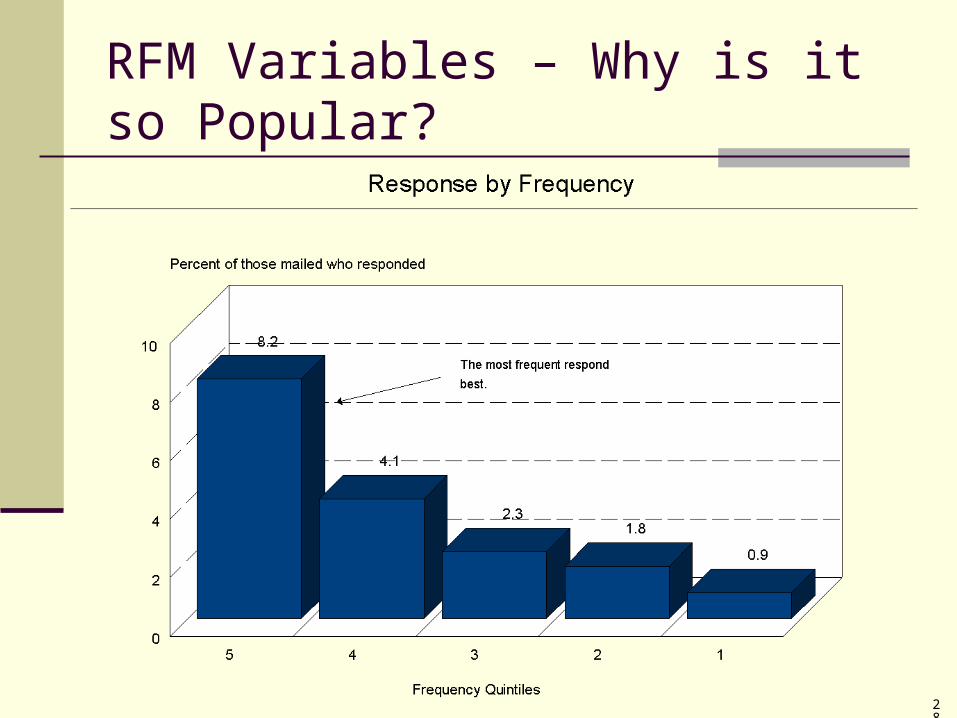
RFM Variables – Why is it so Popular?
1 2 3 4 5
“The people most likely to respond to a new offer are those people who have made a purchase from you most recently”, Arthur Middleton Hughes
28
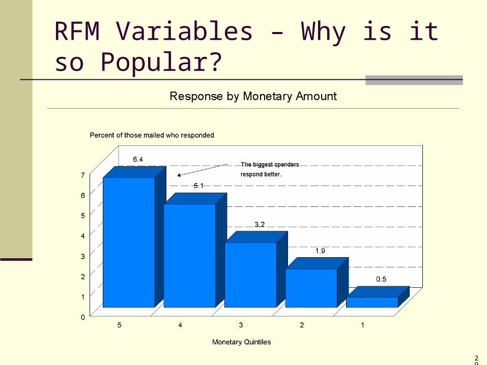
RFM Variables – Why is it so Popular?
29
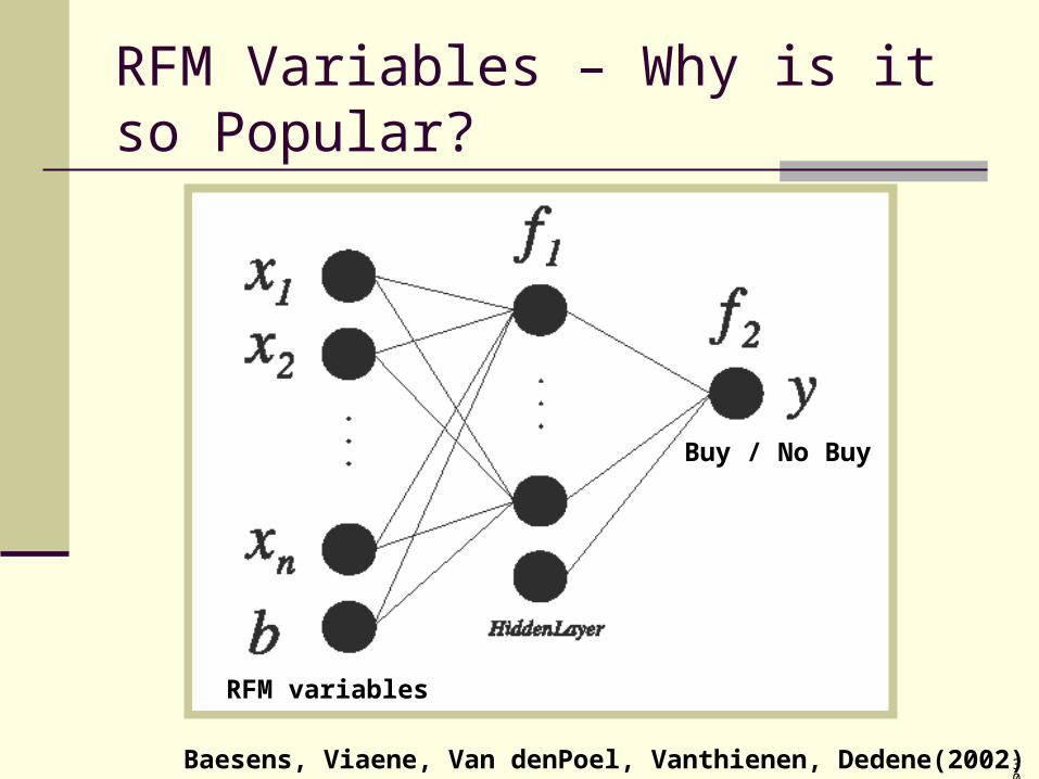
RFM Variables – Why is it so Popular?
30
RFM Variables – Why is it so Popular?
Baesens, Viaene, Van denPoel, Vanthienen, Dedene(2002)
RFM variables
Buy / No Buy
31
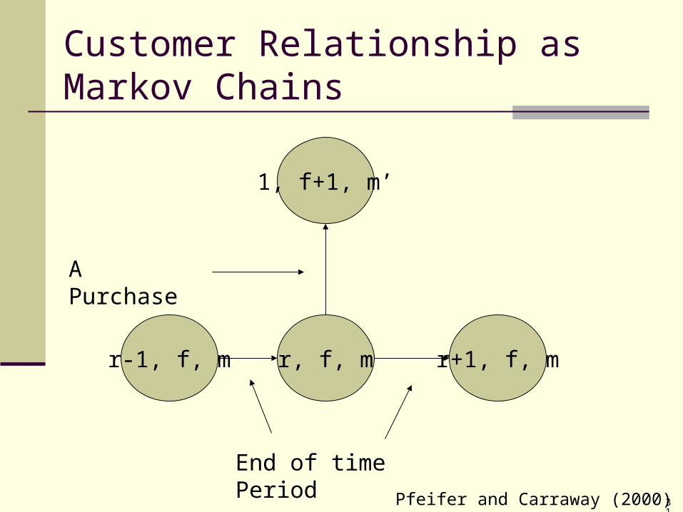
Customer Relationship as Markov Chains
r, f, mr-1, f, m r+1, f, m
1, f+1, m’
End of time Period
A Purchase
Pfeifer and Carraway (2000)
32
Customer Relationship as Markov Chains
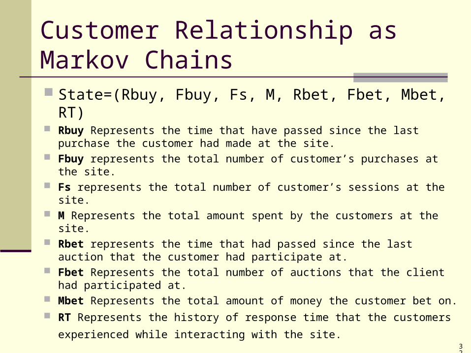
State=(Rbuy, Fbuy, Fs, M, Rbet, Fbet, Mbet, RT) Rbuy Represents the time that have passed since the last purchase
the customer had made at the site. Fbuy represents the total number of customer’s purchases at the
site. Fs represents the total number of customer’s sessions at the site. M Represents the total amount spent by the customers at the site. Rbet represents the time that had passed since the last auction that
the customer had participate at. Fbet Represents the total number of auctions that the client had
participated at. Mbet Represents the total amount of money the customer bet on. RT Represents the history of response time that the customers
experienced while interacting with the site.
33
Customer Relationship as Markov Chains
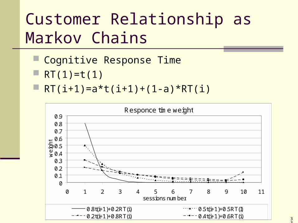
Cognitive Response Time RT(1)=t(1) RT(i+1)=a*t(i+1)+(1-a)*RT(i)
Responce time weight
00.10.20.30.40.50.60.70.80.9
0 1 2 3 4 5 6 7 8 9 10 11sessions number
we
igh
t
0.8t(i+1)+0.2RT(i) 0.5t(i+1)+0.5RT(I)0.2t(i+1)+0.8RT(i) 0.4t(i+1)+0.6RT(i)
34
Customer Relationship as Markov Chains
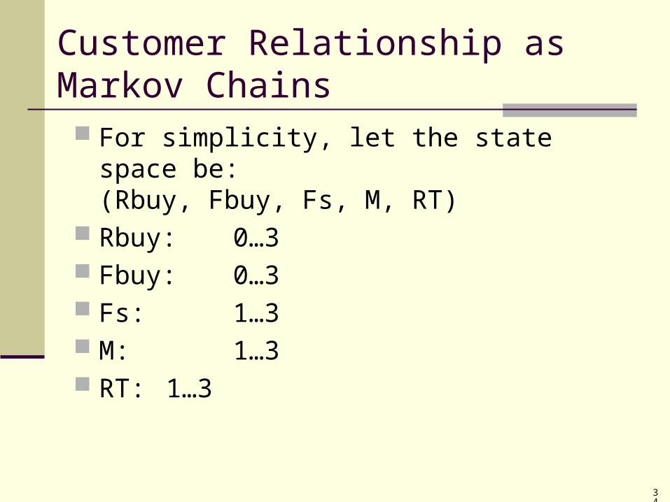
For simplicity, let the state space be:(Rbuy, Fbuy, Fs, M, RT)
Rbuy: 0…3 Fbuy:0…3 Fs: 1…3 M: 1…3 RT: 1…3
35
Customer Relationship as Markov Chains
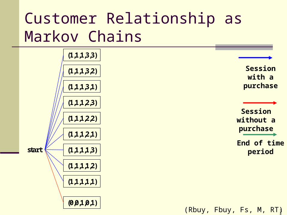
Session with a purchase
Session without a purchase
End of time periodstart
(0,0,1,0,1)
(1,1,1,1,1)
(1,1,1,1,2)
(1,1,1,1,3)
(1,1,1,2,1)
(1,1,1,2,2)
(1,1,1,2,3)
(1,1,1,3,1)
(1,1,1,3,2)
(1,1,1,3,3)
(Rbuy, Fbuy, Fs, M, RT)
36
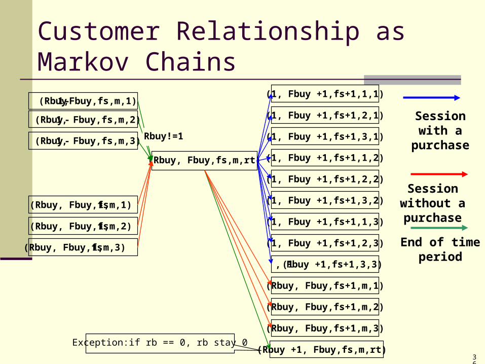
Customer Relationship as Markov Chains
(Rbuy, Fbuy,fs,m,rt)
(1, Fbuy +1,fs+1,1,1)
(1, Fbuy +1,fs+1,2,1)
(1, Fbuy +1,fs+1,3,1)
(1, Fbuy +1,fs+1,1,2)
(1, Fbuy +1,fs+1,2,2)
(1, Fbuy +1,fs+1,3,2)
(1, Fbuy +1,fs+1,1,3)
(1, Fbuy +1,fs+1,2,3)
(1, Fbuy +1,fs+1,3,3)
(Rbuy +1, Fbuy,fs,m,rt)
(Rbuy, Fbuy,fs+1,m,1)
(Rbuy, Fbuy,fs+1,m,2)
(Rbuy, Fbuy,fs+1,m,3)
(Rbuy-1,Fbuy,fs,m,1)
(Rbuy -1, Fbuy,fs,m,2)
(Rbuy -1, Fbuy,fs,m,3) Rbuy!=1
(Rbuy, Fbuy,fs-1,m,1)
(Rbuy, Fbuy,fs-1,m,2)
(Rbuy, Fbuy,fs-1,m,3)
Exception:if rb == 0, rb stay 0
Session with a purchase
Session without a purchase
End of time period
37
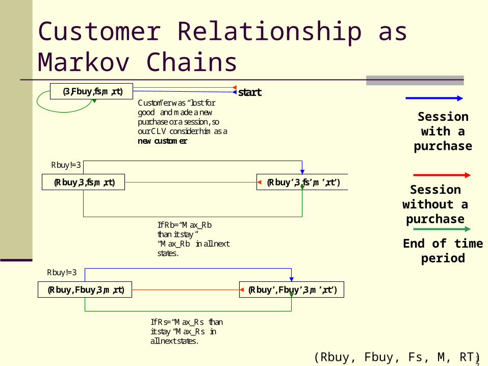
Customer Relationship as Markov Chains
(Rbuy,3,fs,m,rt)
Rbuy!=3
(Rbuy’,3,fs’,m’,rt’)
If Rb=“Max_Rb” than it stay “Max_Rb” in all next states.
(Rbuy, Fbuy,3,m,rt)
Rbuy!=3
(Rbuy’, Fbuy’,3,m’,rt’)
If Rs=“Max_Rs” than it stay “Max_Rs” in all next states.
(3,Fbuy,fs,m,rt) start Customer was “lost for good” and made a new purchase or a session, so our CLV consider him as a new customer
Session with a purchase
Session without a purchase
End of time period
(Rbuy, Fbuy, Fs, M, RT)
38
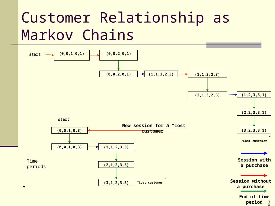
Customer Relationship as Markov Chains
start (0,0,1,0,1) (0,0,2,0,1)
(0,0,2,0,1) (1,1,3,2,3) (1,1,3,2,3)
(2,1,3,2,3) (1,2,3,3,1)
(2,2,3,3,1)
(3,2,3,3,1)
“Lost customer”
start
(0,0,1,0,3)
(0,0,1,0,3) (1,1,2,3,3)
(2,1,2,3,3)
(3,1,2,3,3) “Lost customer”
New session for a “lost customer”
Time periods Session with a purchase
Session without a purchase
End of time period
39
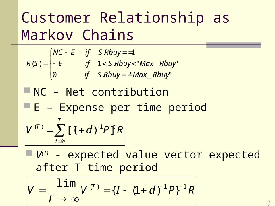
Customer Relationship as Markov Chains
"_".0
"_".1
1.
)(
RbuyMaxRbuySif
RbuyMaxRbuySifE
RbuySifENC
SR
NC – Net contribution E – Expense per time period
RPdV tT
t
T ])1[(0
1)(
V(T) - expected value vector expected after T time period
RPdIVT
V T 11)( })1({lim
40
Experimental
Data were obtained from an E-commerce company in Israel
70,134 purchases (“auction wins”) and 253,736 bets took place, and the total amount of 84,000,000 new Israeli shekels was spent.
41
Experimental
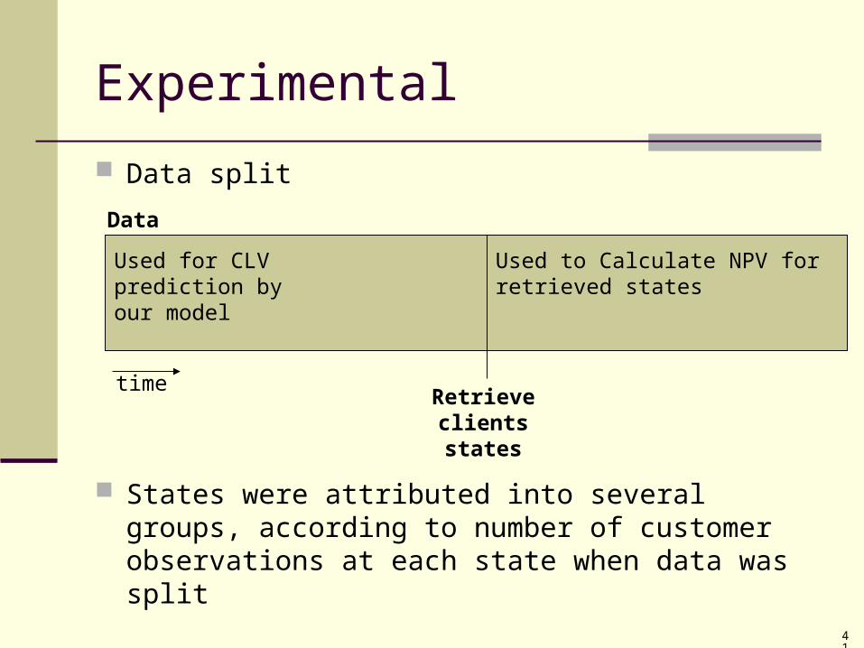
Data split
States were attributed into several groups, according to number of customer observations at each state when data was split
Data
Used for CLV prediction by our model
Used to Calculate NPV for retrieved states
Retrieve clients states
time
42
Experimental
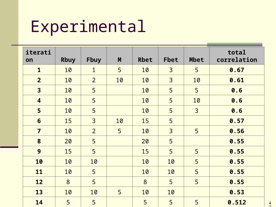
iteration Rbuy Fbuy M Rbet Fbet Mbet total correlation
1 10 1 5 10 3 5 0.67
2 10 2 10 10 3 10 0.61
3 10 5 10 5 5 0.6
4 10 5 10 5 10 0.6
5 10 5 10 5 3 0.6
6 15 3 10 15 5 0.57
7 10 2 5 10 3 5 0.56
8 20 5 20 5 0.55
9 15 5 15 5 5 0.55
10 10 10 10 10 5 0.55
11 10 5 10 10 5 0.55
12 8 5 8 5 5 0.55
13 10 10 5 10 10 0.53
14 5 5 5 5 5 0.512
43
Experimental
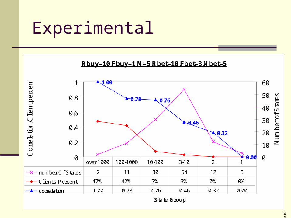
Rbuy=10,Fbuy=1,M=5,Rbet=10,Fbet=3,Mbet=5
1.00
0.78 0.76
0.46
0.32
0.000
0.2
0.4
0.6
0.8
1
State Group
Co
rre
latio
n/C
lien
t pe
rce
nt
0
10
20
30
40
50
60
Nu
mb
er
of S
tate
s
number Of States 2 11 30 54 12 3
Client's Percent 47% 42% 7% 3% 0% 0%
correlation 1.00 0.78 0.76 0.46 0.32 0.00
over 1000 100-1000 10-100 3-10 2 1
44
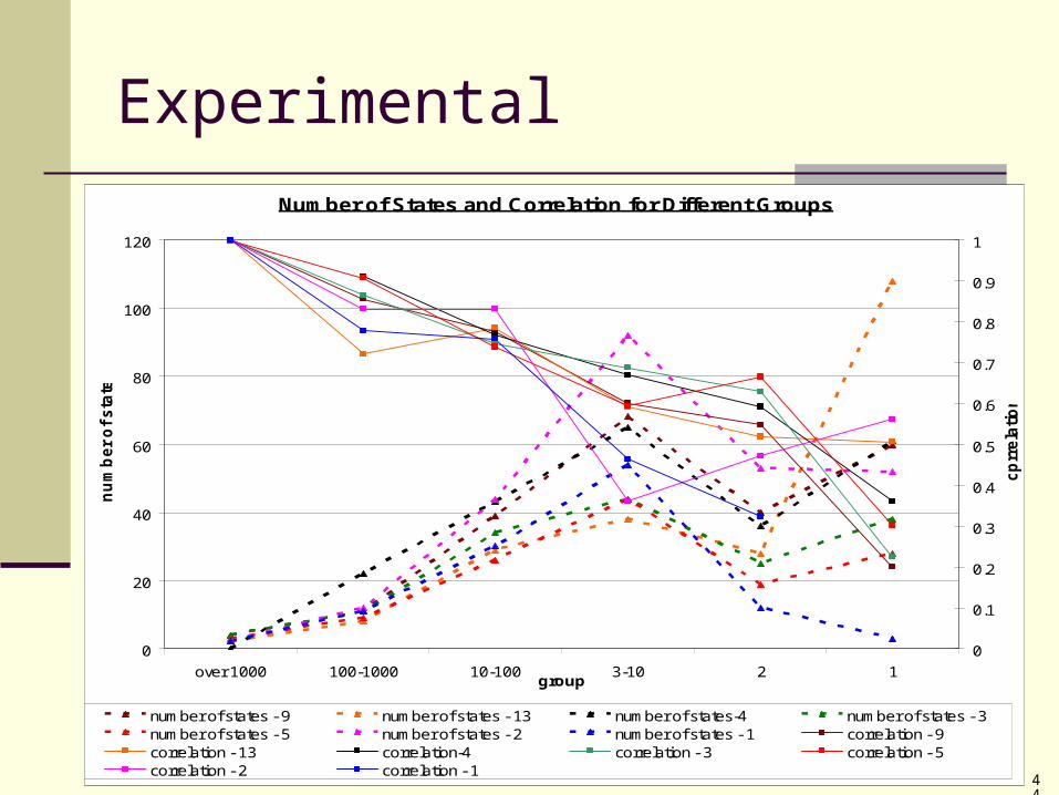
ExperimentalNumber of States and Correlation for Different Groups
0
20
40
60
80
100
120
over 1000 100-1000 10-100 3-10 2 1group
nu
mb
er
of
sta
tes
0
0.1
0.2
0.3
0.4
0.5
0.6
0.7
0.8
0.9
1
cp
rre
lati
on
number of states - 9 number of states - 13 number of states-4 number of states - 3number of states - 5 number of states - 2 number of states - 1 correlation - 9correlation - 13 correlation-4 correlation - 3 correlation - 5correlation - 2 correlation - 1
45
Experimental - Conclusions
High correlation is achieved for state groups where the number of observation per state is high
Criteria for evaluating the model must be defined in order to evaluate the iterations results
A. Total correlation B. Correlation between most popular states C. Group’s correlation with reference to number of states in each
group
46
Experimental - Conclusions
Model must be fitted for additional different domains.
Using visualization techniques and “data cleaning” can help finding the accurate parameters for the model.
Problem: No Data for validating RT and Fs variables.Solutions: Simulation
47
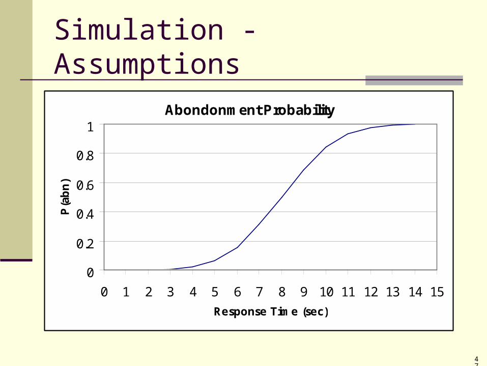
Simulation - Assumptions
Abondonment Probability
0
0.2
0.4
0.6
0.8
1
0 1 2 3 4 5 6 7 8 9 10 11 12 13 14 15
Response Time (sec)
P(a
bn
)
48
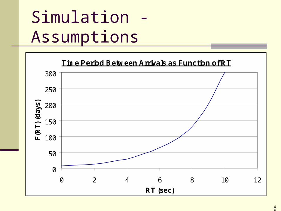
Simulation - Assumptions
Time Period Between Arrivals as Function of RT
0
50
100
150
200
250
300
0 2 4 6 8 10 12
RT (sec)
F(R
T)
(day
s)
49
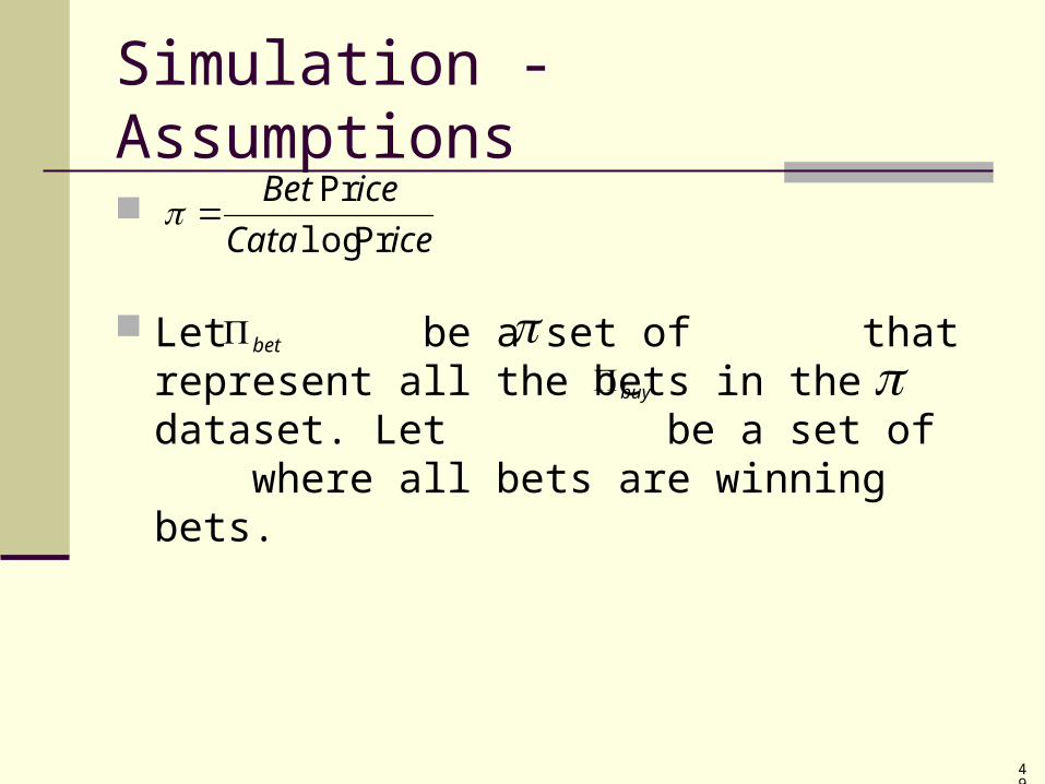
Simulation - Assumptions
Let be a set of that represent all the bets in the dataset. Let be a set of where all bets are winning bets.
iceCata
iceBet
Prlog
Pr
bet buy
50
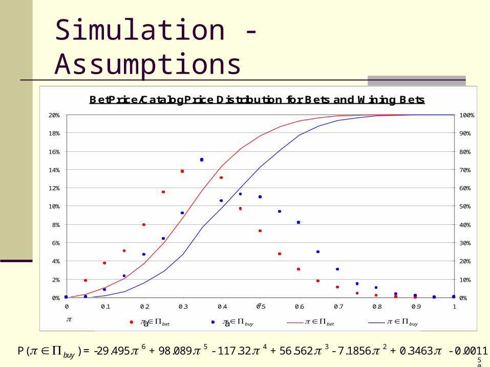
Simulation - Assumptions
BetPrice/CatalogPrice Distribution for Bets and Wining Bets
0%
2%
4%
6%
8%
10%
12%
14%
16%
18%
20%
0 0.1 0.2 0.3 0.4 0.5 0.6 0.7 0.8 0.9 10%
10%
20%
30%
40%
50%
60%
70%
80%
90%
100%
a a a abet buybet buy
P( buy ) = -29.495 6 + 98.089 5 - 117.32 4 + 56.562 3 - 7.1856 2 + 0.3463 - 0.0011
51
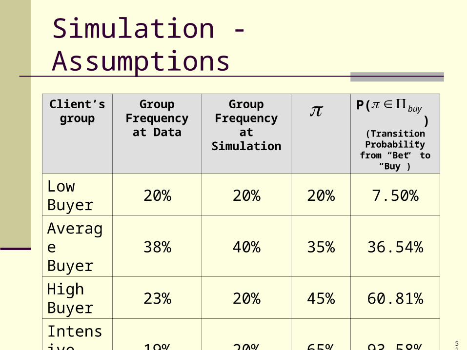
Simulation - Assumptions
P(buyClient’s group
Group Frequency at
Data
Group Frequency at Simulation
P( )(Transition
Probability from “Bet” to “Buy”)
Low Buyer
20% 20% 20% 7.50%
Average Buyer
38% 40% 35% 36.54%
High Buyer
23% 20% 45% 60.81%
Intensive Buyer
19% 20% 65% 93.58%
buy
52
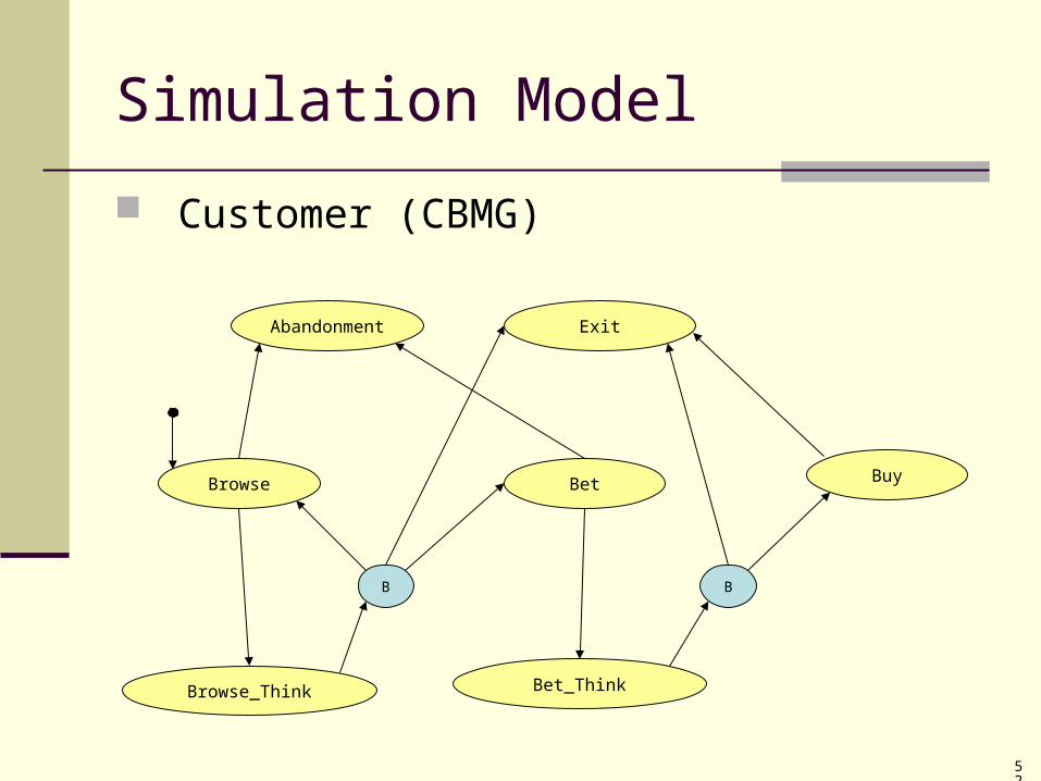
Simulation Model
Browse Bet Buy
Browse_Think Bet_Think
B B
Abandonment Exit
Customer (CBMG)
53
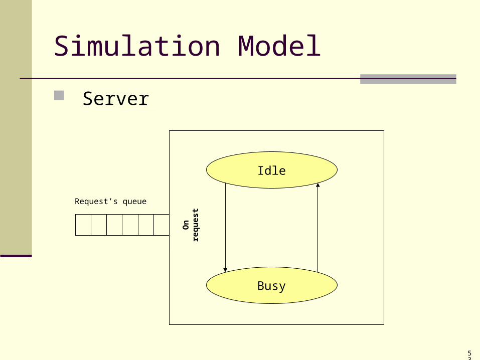
Simulation Model
Server
Idle
Busy
On
re
qu
es
tRequest’s queue
54
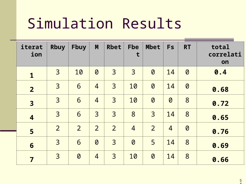
Simulation Results
iteration Rbuy Fbuy M Rbet Fbet Mbet Fs RT total correlation
1 3 10 0 3 3 0 14 0 0.4
2 3 6 4 3 10 0 14 0 0.68
3 3 6 4 3 10 0 0 8 0.72
4 3 6 3 3 8 3 14 8 0.65
5 2 2 2 2 4 2 4 0 0.76
6 3 6 0 3 0 5 14 8 0.69
7 3 0 4 3 10 0 14 8 0.66
55
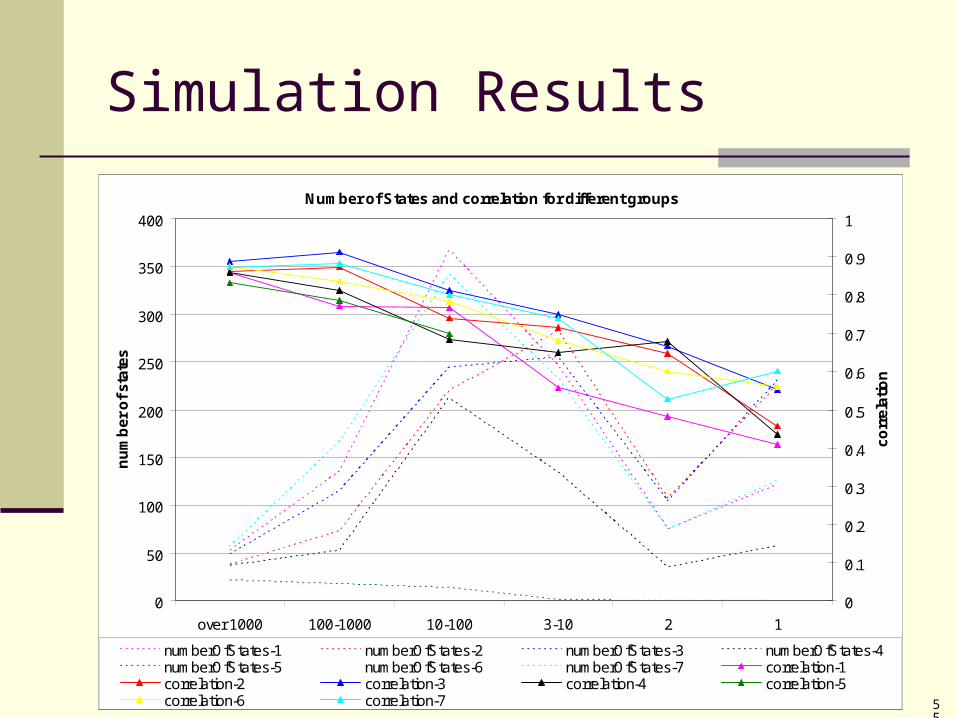
Simulation Results
Number of States and correlation for different groups
0
50
100
150
200
250
300
350
400
over 1000 100-1000 10-100 3-10 2 1
nu
mb
er
of
sta
tes
0
0.1
0.2
0.3
0.4
0.5
0.6
0.7
0.8
0.9
1
co
rre
lati
on
numberOfStates-1 numberOfStates-2 numberOfStates-3 numberOfStates-4numberOfStates-5 numberOfStates-6 numberOfStates-7 correlation-1correlation-2 correlation-3 correlation-4 correlation-5correlation-6 correlation-7
56
Simulation- Conclusions
The model succeeds to predict the influence of bad response time on customer’s value
The CLV model gives better estimation for customer behavior (and lifetime value) if customer behavior is affected by server performance.
57
Future Work
Design a schedule mechanism for the site infrastructure, based on CLV.
Compare this mechanism to the basic FCFS policy and to other priority based mechanisms.
Understanding the marketing outcomes result from the changes in the scheduling policy.