Embed Size (px)
Citation preview

The Algorithmic Foundations of Adaptive Data Analysis October 13, 2017
Lecture 7–10: Stability and Adaptive Analysis ILecturer: Adam Smith Scribe: Adam Smith
So far, we’ve seen that mechanisms whose output is compressible do not allow overfitting: if themechanism’s output is compressible to b bits then, for any given (deterministic) analyst, there are atmost 2b sets of queries that can actually arise, and we can take a union bound over all k · 2b queries thatthe analyst could ever make to get a bound on how much those queries’ empirical means can deviatefrom their population means.
We’ll see at least three other general approaches to limiting the bias over selected analyses: stability-based techniques, information bounds (which encompass compression and, to some extent, stability) andexplicit conditioning. We’ll start with stability, which provides a different formalism for limiting howthe data can affect the output of an algorithm.
1 Algorithmic Stability
We’ll start with the case of classification, and an application that is not directly about adaptivity.Suppose we have an algorithm M that takes a data set s = ((x1, y1), ..., (xn, yn)) of labeled pairs in thedomain X = X ′×0, 1 and outputs a hypothesis h : X ′ → [0, 1] that associates, to every possible futurepoint x, a probability that it should be labeled “1”.
Definition 1 A deterministic algorithm M is ε-uniform change-one (ε-UCO) stable if for all data sets and s′ that differ in one element, and for all inputs z ∈ X ′,
|hs(z)− hs′(z)| ≤ ε where hs = M(s) and hs′ = M(s′) .
A classic example of a stable classification algorithm is the k-nearest neighbors classifier (t-NN). Herethe example domain X ′ is Rd for some finite d. Given a data set and a new point, we classify the pointusing the average of its t nearest neighbors’ labels:
Algorithm 1: t-NN(s, z)
Input: s = (xi, yi)i=1,...,n is a collection of pairs in Rd × 0, 1;z ∈ Rd is a point to be classified.
1 Let i1, ..., it be the indices of the t points in s that are nearest to z(that is, that minimize ‖z − xi‖, breaking ties arbitrarily);
2 return hs(z) = 1k
∑tj=1 yij
Proposition 2 t-NN classification is 1t -UCO stable.
Proof For every fixed point x and data set s, changing a point in s changes at most one of the tnearest neighbors, so the average label can go up or down by at most 1/t.
Recall that we would ideally like to the accuracy of a classifier with respect to fresh samples fromthe underlying distribution. For a classifier that makes “soft” predictions (i.e. outputs a probability in[0, 1]), a simple measure is the expected absolute error:
accD(h)def= 1− E
(x,y)∼D(|y − hs(x)|) .
As in Lecture 3, we’ll use accs(h) to denote the classifier’s empirical accuracy.
accs(h) = 1− 1
n
n∑i=1
(|yi − hs(xi)|) .
7–10-1

Theorem 3 Let M be ε-uniform leave-one-out hypothesis stable. For every data distribution D overlabeled pairs in X × 0, 1, the expected generalization error of the classifier is at most ε, that is:∣∣∣ E
s∼Dn
(accs(hs)− accD(hs)
)∣∣∣ ≤ εWhy is this useful? The algorithm can, in a sense, check its own work: If the NN classifier does well
on the data it was handed, then (for sufficiently large t) it will also do well on future unseen examplesfrom the same distribution.Remark For readers familiar with uniform convergence and VC dimension: A statement like Theo-rem 3 would follow directly from standard tools if the family of classifiers produced by NN were boundedin VC dimension. However, it is not, and there is no reason to think that it would satisfy uniform conver-gence over the entire family of classifiers. Rather, the theorem shows that the classiifer that is actuallyoutput will do approximately as well on fresh samples as it does on the data .
For the proof we introduce additional notation that will be helpful below. Given a data set s, and aposition i, let s−i denote the data set from which s’s ith entry has been removed and let si→x′ denotethe data set in which the ith entry of s has been replaced by a new value x′.Proof The theorem asks us to bound an absolute value; we’ll prove only the upper bound, since thelower bound is symmetric.
Es∼Dn
(accs(hs)− accD(hs)
)=
1
n
n∑i=1
Es∼Dn
(x,y)∼D
|yi − hs(xi)| − Es∼Dn
(x,y)∼D
|y − hs(x)|) (1)
Here is where we will pull the big switch. In the expressions above, the joint distribution on s, (x, y)consists of a sample of n + 1 points drawn i.i.d from D. So in the second expectation, we can swap(xi, yi) and (x, y) without changing the distribution of the random variable.
Es∼Dn
(x,y)∼D
|y−hs(x)|)
= Es∼Dn
(x,y)∼D
|yi−hsi→(x,y)(xi)|
)← (“The switch.” Watch the prover’s hands carefully.)
(2)Substituting this back into the Equation (1), and combining the two expectations, we get
Es∼Dn
(accs(hs)− accD(hs)
)=
1
n
n∑i=1
Es∼Dn
(x,y)∼D
(|yi − hs(xi)| − |yi − hsi→(x,y)
(xi)|)
≤ 1
n
n∑i=1
Es∼Dn
(x,y)∼D
(|hs(xi)− hsi→(x,y)
(xi)|)
(3)
We have passed from evaluating the same classifier hs on two different data sources(either s or fresh samples) to evaluating different classifiers (generated from either s or si→(x,y)) onthe same data point (xi, yi). We can now invoke ε-UCO stability: changing one point in s changesthe classifier’s prediction by at most ε. Hence
Es∼Dn
(accs(hs)− accD(hs)
)≤ 1
n
n∑i=1
Es∼Dn
(x,y)∼D
(ε)
= ε .
Similarly, we can prove the symmetric lower bound: Es∼Dn
(accs(hs)− accD(hs)
)≥ −ε.
7–10-2

2 Distributional Stability
Let’s return to the adaptive setting. There are now two algorithms involved: the mechanism and theanalyst. Together they generate queries based on the data. We’d love to have guarantees along the linesof Theorem 3, but for that we would need the mechanism-analyst pair to be
Can we ever guarantee that the algorithm and mechanism together satisfy stability? Even if themechanism itself is stable (say, for example, it releases a nearest neighbor classifier), the effect of theanalyst may destroy that stability (for example, it could read the description of s embedded in the NNclassifier and output an arbitrary function of the data). The key is to find a notion of stability thatsatisfies postprocessing, as did our notion of compressibility (c.f. Lecture 5). We want that if M is stable,then so is A M , regardless of how A works. We can do this if we switch to randomized mechanisms,and consider the stability of the distribution on outputs of the mechanism.
2.1 Comparing probability distributions
To do this, we’ll need a way to measure how far apart two probability distributions are. We will in factuse multiple measures in this course. Suppose we have distributions P and Q on some set Y. We assumethat P and Q share the same “σ-algebra”, or set of events for which probabilities are defined.
2.1.1 Total Variation Distance
The total variation distance (also called statistical difference or half of the L1 distance) is dTV (P,Q)def=
supE⊆Y |P (E)−Q(E))|. That is, When P and Q are discrete or have well-defined densities, we have
dTV (P,Q)def= sup
E⊆Y|P (E)−Q(E))|
=
∫y:P (y)>Q(y)
|P (y)−Q(y)|dy︸ ︷︷ ︸Area a in figure
=
∫y:P (y)<Q(y)
|P (y)−Q(y)|dy︸ ︷︷ ︸Area b in figure
=1
2
∫y∈Y|P (y)−Q(y)|dy︸ ︷︷ ︸
a+b
. (4)
To see why the first equality holds, notice that the event E that maximizes P (E)−Q(E) includes exactlythe set of points y for which P (y) > Q(y) (every such point helps, and other points either hurt or don’thelp). To see the second equality, note that areas a and b in the following figure are identical, since thearea below both curves is equal to both 1− a and 1− b..
9
a b1 – a = 1 – b
P(y) Q(y)
y
The total variation distance is symmetric and always lies in [0, 1]. It also satisfies the triangleinequality: for all distributions P,Q,R, we have dTV (P,R) ≤ dTV (P,Q) + dTV (Q,R).
Exercise 1 Let U[a,b] denote the uniform distribution on the interval [a, b]. Fix ε > 0. How close areU[0,1] and U[ε,1+ε]? [Answer: dTV (U[0,1], U[ε,1+ε]) = ε .]
The total variation ditance has an important operational interpretation. Namle,y imagine a gamebetween two players, Alice and Bob. Alice flips a coin out of Bob’s sight and gets C ∈ Heads, Tails.If C is heads, Alice samples a point Z according to P . If C is tails, she samples Z according to Q. Nowshe shows Z to Bob, and Bob tries to guess C.
Lemma 4 The success probability of Bob’s best strategy in this game is 12 (1 + dTV (P,Q)).
7–10-3
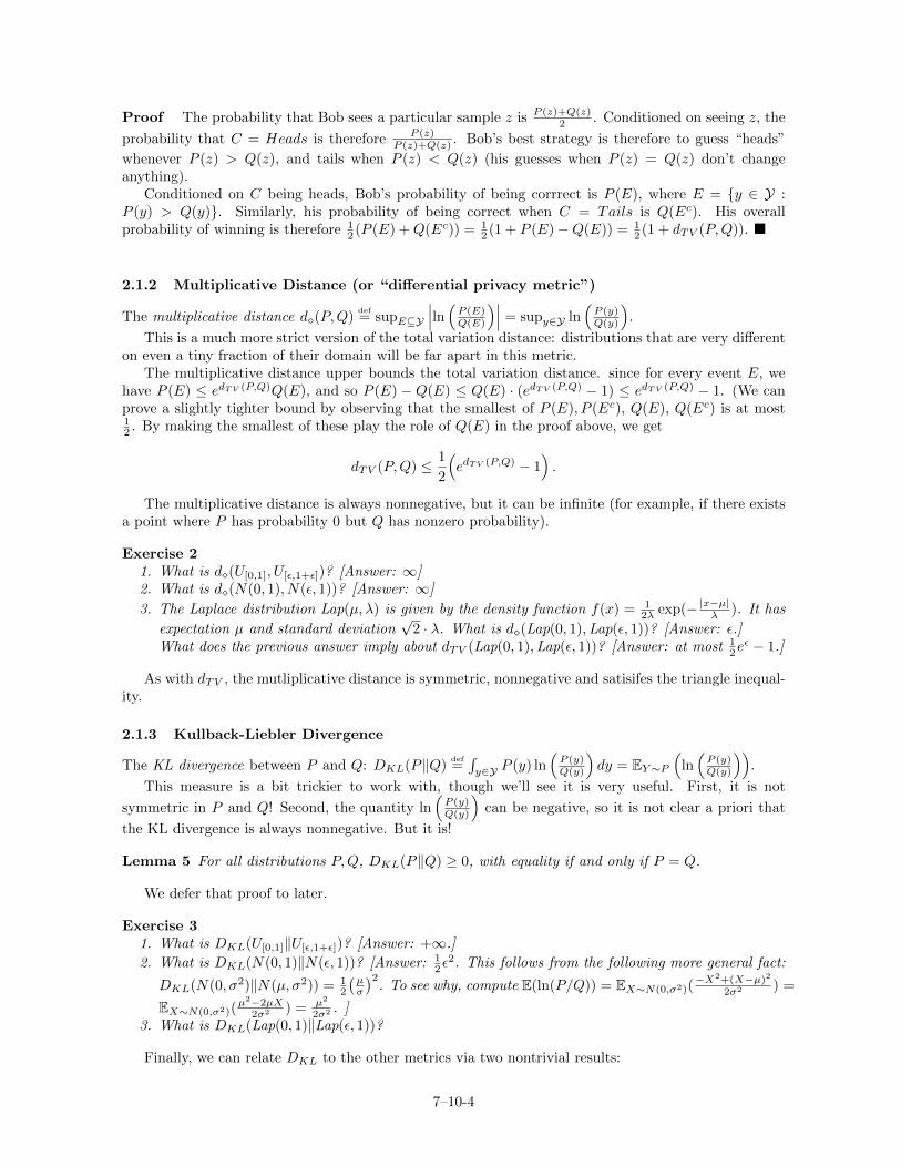
Proof The probability that Bob sees a particular sample z is P (z)+Q(z)2 . Conditioned on seeing z, the
probability that C = Heads is therefore P (z)P (z)+Q(z) . Bob’s best strategy is therefore to guess “heads”
whenever P (z) > Q(z), and tails when P (z) < Q(z) (his guesses when P (z) = Q(z) don’t changeanything).
Conditioned on C being heads, Bob’s probability of being corrrect is P (E), where E = y ∈ Y :P (y) > Q(y). Similarly, his probability of being correct when C = Tails is Q(Ec). His overallprobability of winning is therefore 1
2 (P (E) +Q(Ec)) = 12 (1 + P (E)−Q(E)) = 1
2 (1 + dTV (P,Q)).
2.1.2 Multiplicative Distance (or “differential privacy metric”)
The multiplicative distance d(P,Q)def= supE⊆Y
∣∣∣ln(P (E)Q(E)
)∣∣∣ = supy∈Y ln(P (y)Q(y)
).
This is a much more strict version of the total variation distance: distributions that are very differenton even a tiny fraction of their domain will be far apart in this metric.
The multiplicative distance upper bounds the total variation distance. since for every event E, wehave P (E) ≤ edTV (P,Q)Q(E), and so P (E) − Q(E) ≤ Q(E) · (edTV (P,Q) − 1) ≤ edTV (P,Q) − 1. (We canprove a slightly tighter bound by observing that the smallest of P (E), P (Ec), Q(E), Q(Ec) is at most12 . By making the smallest of these play the role of Q(E) in the proof above, we get
dTV (P,Q) ≤ 1
2
(edTV (P,Q) − 1
).
The multiplicative distance is always nonnegative, but it can be infinite (for example, if there existsa point where P has probability 0 but Q has nonzero probability).
Exercise 21. What is d(U[0,1], U[ε,1+ε])? [Answer: ∞]2. What is d(N(0, 1), N(ε, 1))? [Answer: ∞]
3. The Laplace distribution Lap(µ, λ) is given by the density function f(x) = 12λ exp(− |x−µ|λ ). It has
expectation µ and standard deviation√
2 · λ. What is d(Lap(0, 1),Lap(ε, 1))? [Answer: ε.]What does the previous answer imply about dTV (Lap(0, 1),Lap(ε, 1))? [Answer: at most 1
2eε − 1.]
As with dTV , the mutliplicative distance is symmetric, nonnegative and satisifes the triangle inequal-ity.
2.1.3 Kullback-Liebler Divergence
The KL divergence between P and Q: DKL(P‖Q)def=∫y∈Y P (y) ln
(P (y)Q(y)
)dy = EY∼P
(ln(P (y)Q(y)
)).
This measure is a bit trickier to work with, though we’ll see it is very useful. First, it is not
symmetric in P and Q! Second, the quantity ln(P (y)Q(y)
)can be negative, so it is not clear a priori that
the KL divergence is always nonnegative. But it is!
Lemma 5 For all distributions P,Q, DKL(P‖Q) ≥ 0, with equality if and only if P = Q.
We defer that proof to later.
Exercise 31. What is DKL(U[0,1]‖U[ε,1+ε])? [Answer: +∞.]
2. What is DKL(N(0, 1)‖N(ε, 1))? [Answer: 12ε
2. This follows from the following more general fact:
DKL(N(0, σ2)‖N(µ, σ2)) = 12
(µσ
)2. To see why, compute E(ln(P/Q)) = EX∼N(0,σ2)(
−X2+(X−µ)2
2σ2 ) =
EX∼N(0,σ2)(µ2−2µX
2σ2 ) = µ2
2σ2 . ]3. What is DKL(Lap(0, 1)‖Lap(ε, 1))?
Finally, we can relate DKL to the other metrics via two nontrivial results:
7–10-4
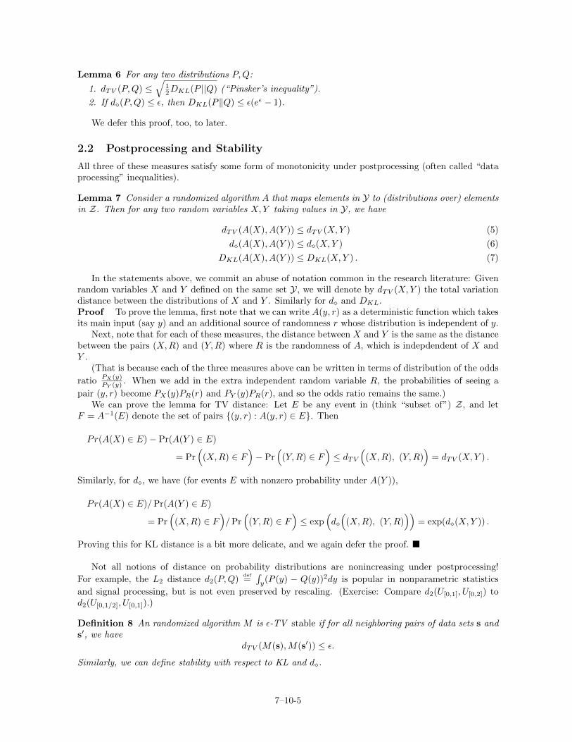
Lemma 6 For any two distributions P,Q:
1. dTV (P,Q) ≤√
12DKL(P ||Q) (“Pinsker’s inequality”).
2. If d(P,Q) ≤ ε, then DKL(P‖Q) ≤ ε(eε − 1).
We defer this proof, too, to later.
2.2 Postprocessing and Stability
All three of these measures satisfy some form of monotonicity under postprocessing (often called “dataprocessing” inequalities).
Lemma 7 Consider a randomized algorithm A that maps elements in Y to (distributions over) elementsin Z. Then for any two random variables X,Y taking values in Y, we have
dTV (A(X), A(Y )) ≤ dTV (X,Y ) (5)
d(A(X), A(Y )) ≤ d(X,Y ) (6)
DKL(A(X), A(Y )) ≤ DKL(X,Y ) . (7)
In the statements above, we commit an abuse of notation common in the research literature: Givenrandom variables X and Y defined on the same set Y, we will denote by dTV (X,Y ) the total variationdistance between the distributions of X and Y . Similarly for d and DKL.Proof To prove the lemma, first note that we can write A(y, r) as a deterministic function which takesits main input (say y) and an additional source of randomness r whose distribution is independent of y.
Next, note that for each of these measures, the distance between X and Y is the same as the distancebetween the pairs (X,R) and (Y,R) where R is the randomness of A, which is indepdendent of X andY .
(That is because each of the three measures above can be written in terms of distribution of the odds
ratio PX(y)PY (y) . When we add in the extra independent random variable R, the probabilities of seeing a
pair (y, r) become PX(y)PR(r) and PY (y)PR(r), and so the odds ratio remains the same.)We can prove the lemma for TV distance: Let E be any event in (think “subset of”) Z, and let
F = A−1(E) denote the set of pairs (y, r) : A(y, r) ∈ E. Then
Pr(A(X) ∈ E)− Pr(A(Y ) ∈ E)
= Pr(
(X,R) ∈ F)− Pr
((Y,R) ∈ F
)≤ dTV
((X,R), (Y,R)
)= dTV (X,Y ) .
Similarly, for d, we have (for events E with nonzero probability under A(Y )),
Pr(A(X) ∈ E)/Pr(A(Y ) ∈ E)
= Pr(
(X,R) ∈ F)/Pr
((Y,R) ∈ F
)≤ exp
(d
((X,R), (Y,R)
))= exp(d(X,Y )) .
Proving this for KL distance is a bit more delicate, and we again defer the proof.
Not all notions of distance on probability distributions are nonincreasing under postprocessing!
For example, the L2 distance d2(P,Q)def=∫y(P (y) − Q(y))2dy is popular in nonparametric statistics
and signal processing, but is not even preserved by rescaling. (Exercise: Compare d2(U[0,1], U[0,2]) tod2(U[0,1/2], U[0,1]).)
Definition 8 An randomized algorithm M is ε-TV stable if for all neighboring pairs of data sets s ands′, we have
dTV (M(s),M(s′)) ≤ ε.
Similarly, we can define stability with respect to KL and d.
7–10-5
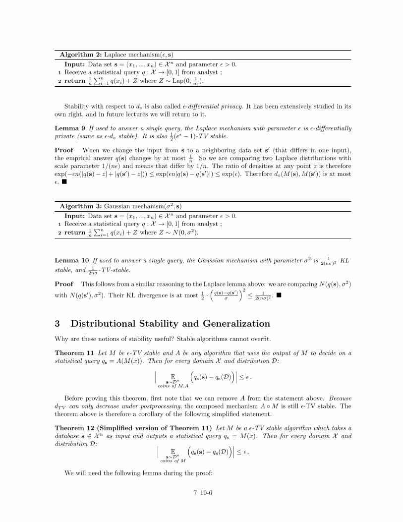
Algorithm 2: Laplace mechanism(ε, s)
Input: Data set s = (x1, ..., xn) ∈ Xn and parameter ε > 0.1 Receive a statistical query q : X → [0, 1] from analyst ;
2 return 1n
∑ni=1 q(xi) + Z where Z ∼ Lap(0, 1
nε ).
Stability with respect to d is also called ε-differential privacy. It has been extensively studied in itsown right, and in future lectures we will return to it.
Lemma 9 If used to answer a single query, the Laplace mechanism with parameter ε is ε-differentiallyprivate (same as ε-d stable). It is also 1
2 (eε − 1)-TV stable.
Proof When we change the input from s to a neighboring data set s′ (that differs in one input),the emprical answer q(s) changes by at most 1
n . So we are comparing two Laplace distributions withscale parameter 1/(nε) and means that differ by 1/n. The ratio of densities at any point z is thereforeexp(−εn(|q(s)− z|+ |q(s′)− z|)) ≤ exp(εn|q(s)− q(s′)|) ≤ exp(ε). Therefore d(M(s),M(s′)) is at mostε.
Algorithm 3: Gaussian mechanism(σ2, s)
Input: Data set s = (x1, ..., xn) ∈ Xn and parameter ε > 0.1 Receive a statistical query q : X → [0, 1] from analyst ;
2 return 1n
∑ni=1 q(xi) + Z where Z ∼ N(0, σ2).
Lemma 10 If used to answer a single query, the Gaussian mechanism with parameter σ2 is 12(nσ)2 -KL-
stable, and 12nσ -TV-stable.
Proof This follows from a similar reasoning to the Laplace lemma above: we are comparingN(q(s), σ2)
with N(q(s′), σ2). Their KL divergence is at most 12 ·(q(s)−q(s′)
σ
)2
≤ 12(nσ)2 .
3 Distributional Stability and Generalization
Why are these notions of stability useful? Stable algorithms cannot overfit.
Theorem 11 Let M be ε-TV stable and A be any algorithm that uses the output of M to decide on astatistical query qs = A(M(x)). Then for every domain X and distribution D:∣∣∣ E
s∼Dn
coins of M,A
(qs(s)− qs(D)
)∣∣∣ ≤ ε .Before proving this theorem, first note that we can remove A from the statement above. Because
dTV can only decrease under postprocessing, the composed mechanism A M is still ε-TV stable. Thetheorem above is therefore a corollary of the following simplified statement.
Theorem 12 (Simplified version of Theorem 11) Let M be a ε-TV stable algorithm which takes adatabase s ∈ Xn as input and outputs a statistical query qs = M(x). Then for every domain X anddistribution D: ∣∣∣ E
s∼Dn
coins of M
(qs(s)− qs(D)
)∣∣∣ ≤ ε .We will need the following lemma during the proof:
7–10-6
Lemma 13 For all X,Y on Y with dTV (X,Y ) ≤ ε, and for all functions f : Y → [0, 1],
|E(f(X))− E(f(Y ))| ≤ ε .
Proof Let PX , PY be the distributions of X,Y respectively.
E(f(X))− E(f(Y )) =
∫f(y)PX(y)dy −
∫f(y)PY (y)dy =
∫f(y)(PX(y)− PY (y))dy
≤∫y:PX(y)>PY (y)
|PX(y)− PY (y)|dy = dTV (X,Y ) . (8)
Proof (of Theorem 12): This proof is almost the same as the proof of Theorem 3. There are a few keydifferences. First, the data points are now abstract values in a domain X ; they need not be example-labelpairs.
Second, the expectation must now be taken over the coins of M in addition to the choice of s andthe new sample x.
The “switch” (Equation (2)) now looks like this:
Es∼Dn
x∼Dcoins of M
(qs(x)
)= E
s∼Dn
x∼Dcoins of M
(qsi→x
(xi))
(9)
Finally, to complete the proof we apply TV stability instead of UCO stability. Analogously toEquation (3), we must bound
Es∼Dn
x∼Dcoins of M
(qs(xi)− qsi→x(xi)
)which we can we rewrite to separate the coins of M :
Es∼Dn
x∼D
(E
coins of Mqs(xi)− E
coins of Mqsi→x
(xi)
).
For fixed xi, the function fxi(q) = q(xi) is a bounded function (that takes a function as input and
returns a value in [0, 1]). Applying Lemma 13 (on how expectations change with changes in dTV ) andthe TV-stability of M , we get that for every s, x ∈ Xn+1, we have
Ecoins of M
qs(xi)− Ecoins of M
qsi→x(xi) ≤ ε .
The remainder of the proof is identical to that of Theorem 3.
This theorem bounds the expected generalization error (difference between empirical mean and pop-ulation mean). But it is more natural to get bounds on the expectation of the absolute value of the error,∣∣∣qs(s) − qs(D)
∣∣∣. With some additional work, one can get the following bound, which we state without
proof:
Theorem 14 Let M be a ε-TV stable algorithm which takes a database s ∈ Xn as input and outputs astatistical query qs = M(x). Then for every domain X and distribution D:
Es∼Dn
coins of M
∣∣∣qs(s)− qs(D)∣∣∣ ≤ ε+ 2√
n.
Exercise 4 1. Show that stability on average over samples in D is sufficient for Theorem 12 : for ssampled i.i.d. from D and s′ obtained by replacing a particular position with a fresh sample fromD, it should hold that the expected TV distance of M(s) and M(s′) is at most ε.
2. Show that Theorem 12 holds for mechanisms that output arbitrary low-sensitivity queries, not onlylinear queries.
7–10-7

“Monitor Argument” [BNSSSU’16]
9
%∗ = %:Q6T:4 ∘ + ∘ %
Monitor(>", (", … , >Y, (Y, b)
1. Find 6∗
= argmax_ (_ − >_ b
2. Return >_∗
S
Mechanism% …
>"("
>#(#
>$($
i.i.d. sample from )
probability distribution on set *
)
Analyst+
Figure 1: The “monitor argument” from the proof of Theorem 15.
3.1 Lifting to Many Rounds via the Monitor Argument
As with compression-based mechanisms, we can combine generalization guarantees with low empiricalerror to get overall error guarantees. The exact argument is different, however. In particular, thereduction from many rounds to a single round has a different flavor.
Theorem 15 (Transfer Theorem for TV-Stable Mechanisms) If M is ε-TV stable and has ex-pected worst case empirical error at most α then, for every distribution D, and for every analyst A,when s ∼ Dn, the expected population error of the mechanism is
Es∼Dn
coins of M,A
(k
maxj=1|aj − qj(D)|
)≤ ε+ α .
Proof We can write bound the total error by the sum of two terms:
kmaxj=1|aj − qj(D)| ≤ k
maxj=1|aj − qj(s)|︸ ︷︷ ︸
empirical error
+k
maxj=1|qj(s)− qj(D)|︸ ︷︷ ︸
generalization error
.
It is tempting to attempt to apply our generalization result directly in order to bound the secondterm. This turns out to be delicate (we will return to it!). Instead, we proceed via a different route.
The idea is to “lift” the bound we have for a single adaptively chosen query to the worst of a set ofqueries by considering a thought experiment. We imagine a new algorithm, called the monitor, whichtakes as input the final conversation q1, a1, ..., qk, ak between M and A, as well as the distribution D.The monitor, illustrated in Figure 1, outputs the name of the query with the worst generalization error:
Monitor(q1, a1, ..., qk, ak,D)def= arg max
j|aj − qj(D)| .
The monitor can only ever be a thought experiment, since it requires knowing the true distribution Din order to pick the worst query.
Let M∗ = MonitorAM be the equally fictional algorithm that takes as input s and the distributionD, runs the interaction between M(s) and A, and runs the monitor (to which it hands D) on the result.Because of closure under postprocessing, M∗ is ε-TV stable. Let j∗ be the number of the query outputby M∗. Since stable algorithms generalize (Theorem 12), we have
E(qj∗(s)− qj∗(D)
)≤ ε.
On the other hand, by the definition of j∗,
maxj
(aj − qj(D)
)= a∗j − qj∗(D) =
(aj∗ − qj∗(s)
)+(qj∗(s)− qj∗(D)
).
7–10-8
The first term on the right-hand side is bounded above by the empirical error, which is at most α inexpectation, by assumption. The second term is the generalization error of M∗, which we just bounded.Taking expectations, we get the desired upper bound, namely:
Emaxj
(aj − qj(D)
)≤ α+ ε .
A symmetric argument shows that Emaxj(qj(D)− aj
)≤ ε+ α.
As a side note, the reduction from many rounds to two rounds via a “monitor” works even withoutan algorithm that is empirically accurate. It requires a slightly more complex monitor which is itselfdistributionally stable. We may return to the proof later in the class. For now we state only the result.
Lemma 16 (Generalization of TV-Stable Mechanisms over Many Rounds) If M is ε-TV sta-ble then, for every distribution D, and for every analyst A, when s ∼ Dn, the expected maximum gener-alization error of the mechanism is
Es∼Dn
coins of M,A
(k
maxj=1|qj(s)− qj(D)|
)≤ ε+
√log k
n.
We will see other uses of the monitor argument later in the course.
4 Composition of distributional notions
We now turn to designing stable algorithms that answer many queries. To do so, we need a compositionstatement analogous to what we had for compressible algorithms. What happens when we chain togetherseveral algorithms that are each distributionally stable? Do stability parameters add up?
Suppose we have an interactive mechanism M that interacts with an analyst over k rounds. We canbreak it into k spearate mechanisms M1,M2, ...Mk, where each of the mechanisms takes as input theoriginal data set s, as well as an internal state (denoted statei), and the query qi. The output nowconsists of the answer ai and the updated internal state statei+1. We call M the adaptive sequentialcomposition of M1, ...,Mk (where “adaptive” comes from the fact that the algorithms’ behavior dependson outcomes of previous rounds).
Theorem 17 (Distributional stability notions compose adaptively) Suppose that M = (M1, ...,Mk).1. Suppose each Mi is ε-TV stable, that is: for every value statei, the randomized map Mi(·, statei)
(which maps s to (ai, statei+1)) is ε-TV stable. Then, for every analyst A, the interactive processA M is kε-TV stable.
2. Suppose that M = (M1, ...,Mk) and each Mi is τ -KL stable. Then, for every analyst A, theinteractive process A M is kτ -KL stable.
3. Suppose that M = (M1, ...,Mk) and each Mi is ε-differentially private (d-stable). Then, for everyanalyst A, the interactive process A M is kε-differentially private.
Proof As with our proof of generalization, using closure under postprocessing, we can reduce thislemma to a simpler statement with no explicit analyst. Consider a sequence of mechanisms M1, ...,Mk,where Mi takes s and the outputs o1, ..., oi−1 of previous mechanisms as input and produces output oi.Now consider the joint output (M1, ...,Mk) obtained by running the mechanisms sequentially.
We prove part (2) of the theorem. We leave parts (1) and (3) as similar exercises.Suppose that Mi(·, o1, ..., oi−1) is τ -KL-stable for every setting of o1, ..., oi−1. To prove part (2) of
the theorem, it is sufficient to prove that M is kτ -KL stable. Fix data sets s, s′ that differ in one input.Let Y1, ..., Yk be the (random) outputs of M on input s, and Z1, ..., ZK be the outputs of M on input s′.
We can write the odds ration Pr(Y=o)Pr(Z=o) as a product
∏j
Pr (Yj=oj |Y j−11 =oj−1
1 )Pr (Zj=oj |Zj−1
1 =oj−11 )
. Thus, the log-odds ratio
is a sum:
lnPr(Y = o)
Pr(Z = o)=
k∑j=1
lnPr(Yj = oj | Y j−1
1 = oj−11
)Pr(Zj = oj | Zj−1
1 = oj−11
) .7–10-9

Taking the expectation over o ∼ Y, we get
DKL(Y ‖Z) =
k∑j=1
Eoj−11 ∼Y j−1
1
(DKL
(Yj∣∣Y j−11 =oj−1
1︸ ︷︷ ︸Mj(oj−1
1 ,s)
∥∥∥Zj∣∣Zj−11 =oj−1
1︸ ︷︷ ︸Mj(oj−1
1 ,s′)
))(10)
Equation (10) is an instance of a general phenomenon, the “chain rule” for KL divergence: giventwo distributions P , Q over pairs of elements, the divergence DKL(P‖Q) is the sum DKL(P1‖Q1) +Ex∼P (DKL(P2,x‖Q2,x)) where P1, Q1 are the marginal distributions of the first element of the pairunder P and Q, respectively, and P2,x, Q2,x are the conditional distributions on the second elementconditioned on the first element being x.
Returning to our proof, the definition of stability says that every divergence on the right-hand sideof (10) is at most τ , so the sum is at most kτ . Hence, M is kτ -KL stable.
Exercise 5 Complete the proofs of parts 1 and 3 of the theorem.
This theorem allows us to analyze complex algorithms and interactive processes modularly.
5 The Gaussian Mechanism
We now turn to our first real application of the machinery we’ve developed for distributionally stablealgorithms.
Theorem 18 The Gaussian mechanism with σ =4√k√
n 4√
log kallows answering k adaptively selected sta-
tistical queries with expected error
O
(4√k log k√n
).
Proof We know that one iteration of the Gaussian mechanism is 12n2σ2 -KL stable. Using the theorem
on adaptive sequential composition, we see that the composed mechanism is k2n2σ2 -KL stable, and hence
√k
2nσ -TV stable (by Pinsker’s inequality). On the other hand, the expected maximum empirical errorof the Gaussian mechanism on a sequence of k queries is O(σ
√log k), since the probability that each
individual query deviates by more that cσ√
log k is e−Ω(c)/k. The overall expected population error isthus
O
(√k
nσ+ σ
√log k
).
Setting σ =4√k√
n 4√
log kyields the desired result.
Note that we could not have gotten this result using only the composition results for TV stability,since those parameters would add up on the “wrong scale”. The Gaussian noise mechanism for a singlequery is 1
2nσ -TV stable. Applying composition for TV stability to the k-query mechanism shows that
the k-query version is k2nσ -TV stable, which is much worse than the
√k
2nσ bound one gets via KL stability.The advantage of working with distributional stability instead of compression bounds is we get much
tighter composition guarantees, often yielding a quadratic improvement in utility. The disadvantage isthat distributionally stable algorithms are more complicated, since they involve extra randomization,and trickier to analyze.
At this point, it is worth asking if one can do can get significantly better error than the bound ofTheorem 18. What is the best possible guarantee for the Gaussian mechanism? Is there any mechanismthat can achieve better guarantees for arbitrary sequences of adaptive queries? We will see a completeanswer to the first, and a partial answer to the second, in the coming lectures.
7–10-10

0 0.8 1.6 2.4
Figure 2: The function f(x) = x ln(x) is strictly convex on (0,∞). The red line shows the linear lowerbound at x = 0.5.
6 Working with divergences
We now tie up our remaining loose ends by proving the required properties of the KL divergence (andintroducing some useful inequalities along the way).
6.1 Jensen’s inequality
Recall from earlier lectures that a set C ⊆ Rd is convex if for every two points x, y ∈ C, the line segmentxy is contained in C. A function f : C → R is convex on C if, at every value x, there is a linear functiontangent to f at x that bounds f below on the whole domain. That is, there exists u ∈ Rd such that forevery y ∈ C, f(y) ≥ f(x) + 〈u, y − x〉. (If f is differentiable, then u is unique and is the gradient ∇f(x);otherwise, the set of vectors u that fit the condition is called the subgradient set of f at x, and denoted∂f(x)). See Figure 6.1.
We say a function is strictly convex if the linear lower bound is strict everywhere except at x. Thatis, for every y ∈ C \ x, we have f(y) > f(x) + 〈u, y − x〉.
If a function is twice differentiable on its domain C, then it is strictly convex if and only if its secondderivative is positive (or positive definite, in dimension greater than 1) on all of C.
Exercise 6 Prove that f(x) = x ln(x) and f(x) = ln(1/x) are both strictly convex on (0,∞).
Lemma 19 (Jensen’s inequality) Let f be a convex function on C ⊆ Rd and X a random variabletaking values in C with finite expectation. Then
f(E(X)) ≤ E(f(X)) .
Furthermore, if f is strictly convex, then we have equality if and only if X is constant (that is, X equalssome particular value with probability 1).
Proof Let µ = E(X) and f(µ) + 〈uµ, y − µ〉 be a linear lower bound to f that is tangent to f at µ.Then
E(f(X)) ≥︸︷︷︸convexity
E(f(µ) + 〈uµ, X − µ〉) =︸︷︷︸linearity
of expectation
f(µ) + 〈uµ,E(X)− µ︸ ︷︷ ︸0
〉 = f(µ).
When f is strictly convex, the first inequality be an equality only when the random variable X places 0probability mass on the set C \ µ (since on that set, f(y) > f(µ) + 〈uµ, y − µ〉). Thus, the inequalityis tight only when X = µ with probability 1.
Using Jensen’s inequality, one can prove the following well known inequality, whose proof is left asan exercise:
7–10-11

Lemma 20 (Log-Sum Inequality) Let a1, . . . , an and b1, . . . , bn be nonnegative numbers. Denote thesum of all ai’s by a and the sum of all bi’s by b. Then
n∑i=1
aia
logaibi≥ log
a
b
with equality if and only if aibi
are equal for all i.
6.2 Basic Properties of KL
We collect here a few properties of KL divergence that we used when discussing stability.
Lemma 21 For every two distributions P and Q on a set X :1. DKL(P‖Q) ≥ 0 with equality if and only if P = Q.2. If d(P,Q) = ε, then DKL(P‖Q) ≤ DKL(PQ) +DKL(Q‖P ) ≤ ε(eε − 1).3. (Chain rule for KL) If X is a product of two sets X1 × X2, (so that P , Q are distributions over
pairs), the divergence DKL(P‖Q) is the sum DKL(P1‖Q1)+Ex∼P (DKL(P2,x‖Q2,x)) where P1, Q1
are the marginal distributions of the first element of the pair under P and Q, respectively, andP2,x, Q2,x are the conditional distributions on the second element conditioned on the first elementbeing x.
4. (Monotonicity under postprocessing) For every randomized map A taking inputs in X ,DKL(A(P )‖A(Q)) ≤ DKL(P‖Q).
5. (Pinsker’s inequality) dTV (P,Q) ≤√
12DKL(P‖Q)
Proof1. DKL(P‖Q) = EX∼P
(ln P (X)
Q(X)
)= EX∼P
(− ln Q(X)
P (X)
). Applying Jensen’s inequality to f(x) =
− ln(x), we get DKL(P‖Q) ≥ − ln(EX∼P
(Q(X)P (X)
)). If we expand the definition of expectation, we
see that the denominator cancels in the expression EX∼P(Q(X)P (X)
), and we have EX∼P
(Q(X)P (X)
)=∫
x∈supp(P )Q(x)P (x)P (x)dx =
∫x∈supp(P )
Q(x) ≤ 1 where supp(P ) is the set of points with positive
density (or mass, in the discrete case). Thus DKL(P‖Q) ≥ 0. We get equality in Jensen’s
inequality if and only if Q(X)P (X) is constant (since − ln(·) is strictly convex). Since P and Q both
integrate to 1, we thus get equality if and only if P = Q.2. By nonnegativity of KL, we have DKL(P‖Q) ≤ DKL(PQ) +DKL(Q‖P ). Expanding the sum, we
have
DKL(PQ) +DKL(Q‖P ) = EX∼P
(ln P (X)
Q(X)
)+ EX∼Q
(ln Q(X)
P (X)
)= EX∼P
(ln P (X)
Q(X) + Q(X)P (X) ln Q(X)
P (X)
)= EX∼P
(1− Q(X)
P (X)
)ln P (X)
Q(X)
≤ EX∼P
(∣∣∣1− Q(X)P (X)
∣∣∣ · ∣∣∣ln P (X)Q(X)
∣∣∣) .Now we can use the fact that d(P,Q) = ε: the term
∣∣∣ln P (X)Q(X)
∣∣∣ in the last expression is always at
most ε, and the term∣∣∣1− Q(X)
P (X)
∣∣∣ is at most max(1− e−ε, eε − 1) = eε − 1. The expectation on the
right-hand side is thus at most ε(eε − 1).3. This is the chain rule for DKL, which we proved when proving the composition lemma. We include
it in this lemma just to have important properties of KL collected in one place.4. First, note that if X and Y are distributed according to P and Q respectively, then the KL
divergence between the distributions of the pairs X,A(X) and Y,A(Y ) is exactly the same asDKL(P‖Q):
DKL
((X,A(X)), (Y,A(Y ))
)= E
x∼Pz∼A(X)
(lnP (x) Pr(z = A(x))
Q(x) Pr(z = A(x))
)= E
x∼Pz∼A(X)
(lnP (x)
Q(x)
)= DKL(P‖Q) .
7–10-12

We can now apply the chain rule:
DKL
((X,A(X)), (Y,A(Y ))
)= DKL(A(X), A(Y )) + E
x∼Pz∼A(x)
DKL
(X∣∣z=A(X)
∥∥Y ∣∣z=A(Y )
)︸ ︷︷ ︸
≥0
.
By the nonnegativity of KL divergence, the expectation on the right-hand side is always nonneg-ative, so we get
DKL(A(X), A(Y )) ≤ DKL
((X,A(X)), (Y,A(Y ))
)≤ DKL(X‖Y ) ,
as desired.5. Recall that dTV (P,Q) = supE |P (E)−Q(E)|. Let E∗ be a fixed event, and let P ′, Q′ be dis-
tributions on 0, 1 with P ′(0) = P (E)def= p and Q′(0) = Q(E)
def= q. Let DKL(p‖q) denote
DKL(P ′‖Q′) ≤ DKL(P‖Q) (since processing can only decrease divergence). Our inequality re-duces to:
DKL(p‖q)− 2(p− q)2 ≥ 0 .
To prove this, fix an arbitrary p ∈ [0, 1] and compute the partial derivative with respect to q:
∂
∂q
(DKL(p‖q)− 2(p− 1)2
)=
q − pq(1− q)
− 4(q − p) = (q − p)(
1q(1−q) − 4
).
Now 1q(1−q) − 4 is never negative (since q(1− q) ≤ 4), so the function g(q) = DKL(p‖q)− 2(p− 1)2
is increasing for q > p and decreasing for q < p. Thus the minimum occurs at q = p, where thefunction is 0.
7 Notes
The stability-based approach to analyzing generalization error dates back to work of Devroye and Wag-ner [DW79]. The topic is now well studied in learning theory–see, for example, Bousquet and Elisseeff[BE02] and Shalev-Shwartz et al. [SSSSS10] for thorough treatments and further references.
The idea of using distributional stability in the context of adaptive statistical queries comes fromDwork et al. [DFH+15]. Theorem 11 was folklore in the differential privacy literature for some time.The first application we are aware of is in [BST14], which used the lemma to relate the empirical errorand generalization error of differentially private learning algorithms.
The presentation of the “monitor” argument comes from Bassily et al. [BNS+16]. The analysis ofthe Gaussian mechanism via KL stability is implicit in [BNS+16] but draws on ideas in Russo andZou [RZ16] and Wang et al. [WLF16].
References
[BE02] Olivier Bousquet and Andre Elisseeff. Stability and generalization. Journal of MachineLearning Research, 2:499–526, 2002.
[BNS+16] Raef Bassily, Kobbi Nissim, Adam D. Smith, Thomas Steinke, Uri Stemmer, and JonathanUllman. Algorithmic stability for adaptive data analysis. In Daniel Wichs and Yishay Man-sour, editors, Proceedings of the 48th Annual ACM SIGACT Symposium on Theory of Com-puting, STOC 2016, Cambridge, MA, USA, June 18-21, 2016, pages 1046–1059. ACM, 2016.
[BST14] Raef Bassily, Adam Smith, and Abhradeep Thakurta. Private empirical risk minimization:Efficient algorithms and tight error bounds. In IEEE Symposium on the Foundations ofComputer Science (FOCS), pages 464–473, 2014.
7–10-13

[DFH+15] Cynthia Dwork, Vitaly Feldman, Moritz Hardt, Toniann Pitassi, Omer Reingold, andAaron Leon Roth. Preserving statistical validity in adaptive data analysis. In STOC, pages117–126. ACM, 2015.
[DW79] L. Devroye and T. Wagner. Distribution-free performance bounds for potential function rules.IEEE Transactions on Information Theory, 25(5):601–604, 1979.
[RZ16] Daniel Russo and James Zou. Controlling bias in adaptive data analysis using informationtheory. In 19th International Conference on Artificial Intelligence and Statistics, pages 1232–1240, 2016. arXiv:1511.05219.
[SSSSS10] S. Shalev-Shwartz, O. Shamir, N. Srebro, and K. Sridharan. Learnability, stability anduniform convergence. JMLR, 2010.
[WLF16] Yu-Xiang Wang, Jing Lei, and Stephen E Fienberg. A minimax theory for adaptive dataanalysis. arXiv:1602.04287 [stat.ML], 2016.
7–10-14