1 About clusters

Although we usually do not realize it, clusters belong to our everyday life. They have beenexploited practically in many situations without people being aware of the underlying details.The tailoring of fine dispersed pieces of material (clusters !) inside bulk has, for example,been turned to an art by craft-workers for centuries. Already the Romans knew, empirically,how to play with the size of dispersed particles in a glass to produce various shining colors.Depending on the size of the gold inclusions, a glass could thus exhibit red as well as yellowreflections, for an example see [KV93]. In a different domain, photography also represents atypical application of cluster physics. Depending on the size of the AgBr clusters depositedon the film, they will more or less quickly and finely respond to light and thus perpetuatethe properties of the produced image. Early photographers of the nineteenth century quicklyrealized and controlled such physical behaviors. Still, even at that time, clusters were notconsidered as objects of scientific studies, even not recognized as specific objects. The workof Mie at the turn of the twentieth century probably constitutes one of the earliest speculationson the existence and specificity of metal clusters — or rather, because the word “cluster” didnot exist in this context at that time, of “small particles” [Mie08]. The question raised by Mieconcerned the response of small metal particles to light, and how this response might dependon the size of the considered particle. Let us quote Mie: “Because gold atoms surely differin their optical properties from small gold spheres”, it would “probably be very interestingto study the absorption of solutions with the smallest submicroscopical particles; thus, in away, one could investigate by optical means how gold particles are composed of atoms”. Anon negligible part of today’s investigations on clusters relies on, or is very close to, Mie’sintuition. As we shall see throughout this book, light represents a particularly useful meansfor the investigation of both structure and dynamics of clusters. And the response of clustersto light is indeed extremely sensitive to their properties. The beautiful achievements of Romanand later glass makers precisely reflect such properties. And photography, as well, is an artdealing with light.

The inspiring intuition of Mie did not suffice to promote cluster science to the status of awell recognized field of physics. Indeed the times of the early twentieth century were busywith the identification and analysis of “elementary” constituents of matter and only simplemolecules seemed in reach of understanding in the mid century, or alternatively the other ex-treme, namely the problem of bulk material, of course with other techniques than the onesused in atomic physics. Modern cluster physics, as we know it today, only appeared in thelast quarter of the twentieth century with the possibility of producing free clusters and track-ing such small particles with several, still developing, techniques. This allowed the initiationof studies on clusters as such, which was an important step for the field. Indeed, embedded

Introduction to cluster dynamics. Paul-Gerhard Reinhard, Eric SuraudCopyright c© 2004 Wiley-VCH Verlag GmbH & Co. KGaA

ISBN: 3-527-40345-0

2 1 About clusters

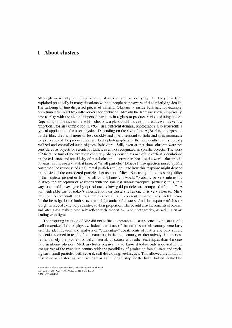
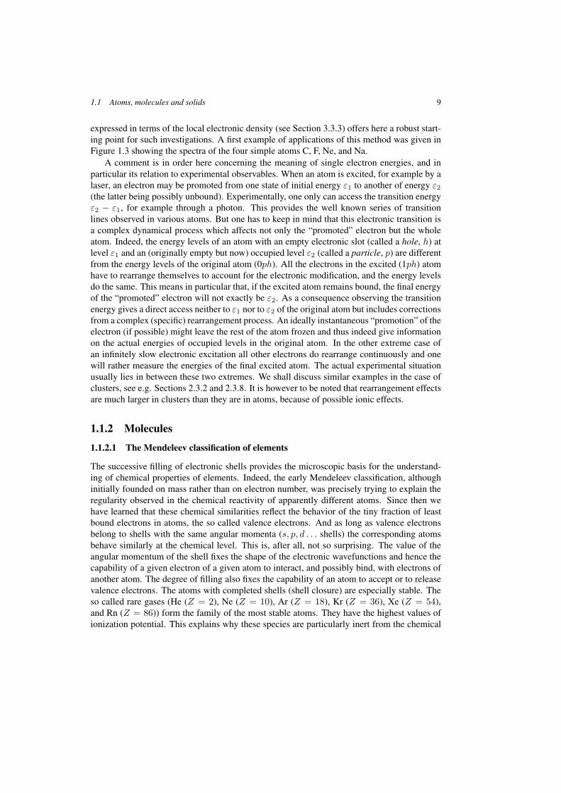
Figure 1.1: Ionic structure of the famous C60 clus-ter. The 60 atoms are arranged as 12 pentagons and20 hexagons yielding a truncated icosahedron. Thatshape consists in 12 vertices bound together by 20equilateral (and equal) triangles. At each vertex ofthe icosahedron, 5 triangles meet. Truncating thesevertices by a plane, leads to the pentagonal faces.The total number of vertices becomes 60. For thisC60, 120 symmetry operations can be identified. Andthis high degree of symmetry has long been used byartists, the actual name of “Buckminster fullerenes”going back to the architect Richard BuckminsterFuller, renowned for his geodesic domes based onpentagons and hexagons.

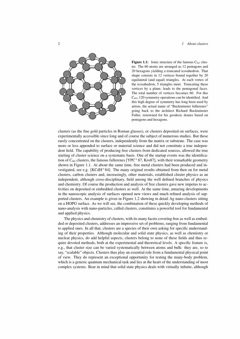
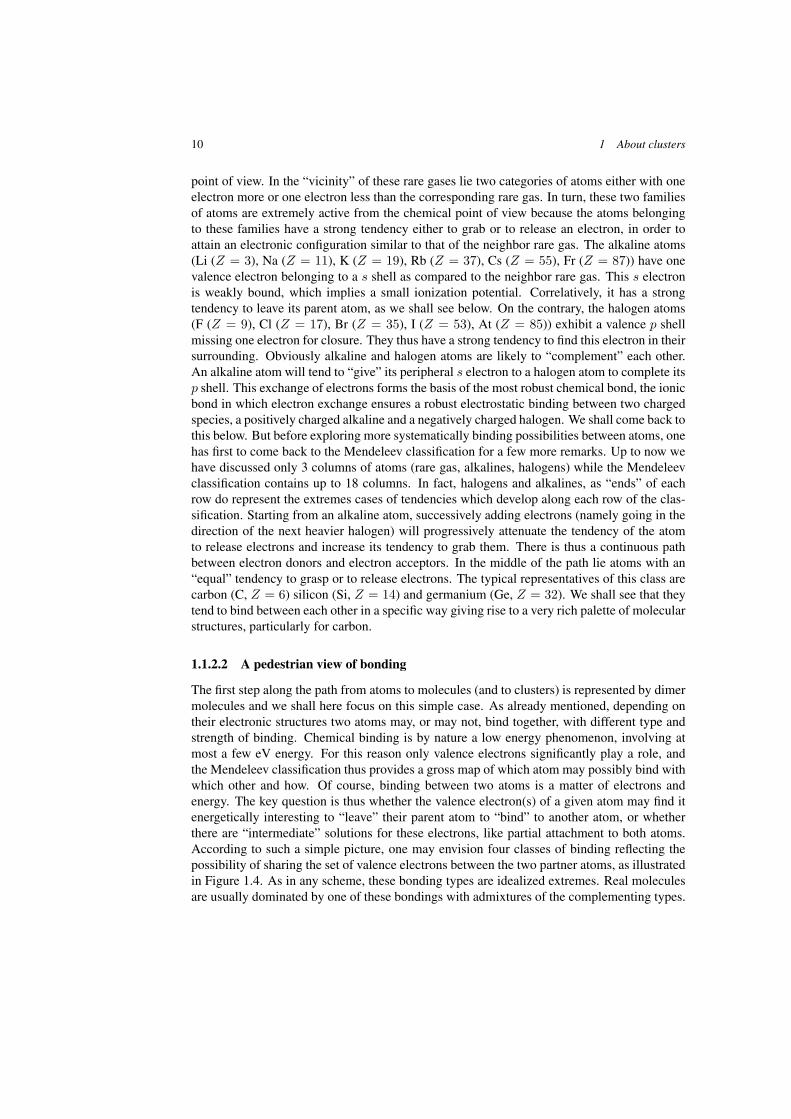
clusters (as the fine gold particles in Roman glasses), or clusters deposited on surfaces, wereexperimentally accessible since long and of course the subject of numerous studies. But theserarely concentrated on the clusters, independently from the matrix or substrate. The case wasmore or less appended to surface or material science and did not constitute a true indepen-dent field. The capability of producing free clusters from dedicated sources, allowed the truestarting of cluster science on a systematic basis. One of the startup events was the identifica-tion of C60 clusters, the famous fullerenes [YPC+87, Kro87], with their remarkable geometryshown in Figure 1.1. At about the same time, free metal clusters had been produced and in-vestigated, see e.g. [KCdH+84]. The many original results obtained from then on for metalclusters, carbon clusters and, increasingly, other materials, established cluster physics as anindependent, although cross-disciplinary, field among the well defined branches of physicsand chemistry. Of course the production and analysis of free clusters gave new impetus to ac-tivities on deposited or embedded clusters as well. At the same time, amazing developmentsin the nanoscopic analysis of surfaces opened new views and much refined analysis of sup-ported clusters. An example is given in Figure 1.2 showing in detail Ag nano-clusters sittingon a HOPG surface. As we will see, the combination of these quickly developing methods ofnano-analysis with nano-particles, called clusters, constitutes a powerful tool for fundamentaland applied physics.

The physics and chemistry of clusters, with its many facets covering free as well as embed-ded or deposited clusters, addresses an impressive set of problems, ranging from fundamentalto applied ones. In all that, clusters are a species of their own asking for specific understand-ing of their properties. Although molecular and solid state physics, as well as chemistry ornuclear physics, do add helpful aspects, clusters belong to none of these fields and thus re-quire devoted methods, both at the experimental and theoretical levels. A specific feature is,e.g., that cluster size can be varied systematically between atoms and bulk: they are, so tosay, “scalable” objects. Clusters thus play an essential role from a fundamental physical pointof view. They do represent an exceptional opportunity for testing the many-body problem,which is a generic quantum mechanical task and lies at the heart of the understanding of mostcomplex systems. Bear in mind that solid state physics deals with virtually infinite, although

1 About clusters 3

Figure 1.2: Topography of silver nanoparticles deposited on highly oriented pyrolytic graphite (HOPG),recorded with an in situ scanning tunneling microscope (STM). From [LMP+00].

symmetric, samples while in molecular or nuclear physics the systems never contain morethan a few hundreds of constituents. Clusters bridge the gap. But the interest in them is notpurely fundamental. As outlined above, clusters play a role in many practical situations likephotography or artwork. More precisely, they have applications in many fields of science as,e.g., astrophysics, chemistry or material science. For example, clusters seem to play an im-portant role in the formation mechanisms and the properties of cosmic dust [CTB89]. Carbonclusters are also expected to be present in the interstellar medium. The most striking prop-erty of clusters for applications in chemistry is their size. Indeed, because clusters may bequite small, but not too small, they can exhibit a large and tunable surface to volume ratio.They may thus provide ideal catalysts and play a crucial role in reaction kinetics [SAH+99].A typical example of application here is photography. In material science, the discovery offullerenes and carbon nanotubes opened the way to the design of new materials [Kai01]. Thisbreakthrough renewed chemistry and physics of carbon to such a level that this field is almostbecoming independent from the mother field of cluster physics, probably in part because ofits many industrial applications.

Cluster physics with its many achievements now belongs to one of the most active fieldsin physics, and offers, through related domains like the physics of nanotubes or fullerenes,one of the fastest developing areas in applied as well as in fundamental science. It is closeto impossible to cover in a single book all the topics related to cluster physics. We shall thusfocus here on one important aspect of the field: cluster dynamics. As in atomic and molecularphysics, detailed studies on the dynamics of quantum many-body systems were boosted bythe rapid progress of laser technology and the possibility of studying electronic motion atthe femtosecond (fs) level. Clusters add to these studies the variability of sizes, as discussed

4 1 About clusters

above. Of course, the field of cluster science is so recent that we shall devote a large part ofthe book to the principle methods of cluster physics, experimental ones (in Chapter 2) as wellas theoretical ones (in Chapter 3). Before that, we are going discuss in this chapter here thenature of clusters in relation to more established objects such as atoms and molecules, on theone side, and bulk, on the other side. Not surprisingly, we shall see that size turns out to bea key quantity, influencing many cluster properties. And we shall see that clusters are morethan just big molecules or “small” pieces of bulk. They are indeed objects of their own, andcluster physics thus has to combine expertise from various fields of physics and chemistry intoan excitingly new area of research.

1.1 Atoms, molecules and solids

Before considering clusters made of atoms, it is useful to briefly summarize what we need toknow on the more “traditional” systems such as atoms, molecules and solids. Clusters rangebetween these extremes and we shall see that understanding binding mechanisms betweenatoms or inside bulk provides the necessary keys to understand binding of clusters. Startingpoint is the atoms, then we discuss their combination in terms of molecules and in the infinitelimit in terms of solids. We can then address clusters. For all species, we give here a briefoverview with bias on the electronic structure, mostly at a qualitative level. For more thoroughdiscussions, we refer the reader to standard textbooks of atomic, molecular, chemical physicsor solid-state physics as cited at the relevant places.

1.1.1 Atoms

1.1.1.1 Qualitative aspects

Atoms consist of a central nucleus and a neutralizing electronic cloud. The atomic number Zlabels the charge of the nucleus which is the number of protons inside the nucleus. The otherconstituents are the neutrons which, however, play a negligible role for the electronic problem,at least at the level we are interested in. For our purpose, we can safely reduce the effect of thenucleus to that of a point charge Ze (thus neglecting hyper-fine structure as effects of finitesize and magnetic coupling [YH96]). Electrons are then supposed to feel only the Coulombfield of the (point-) nucleus. At the level of the fine structure, there are the relativistic effectson the electrons as spin-orbit splitting and Breit interaction [Wei78]. These are, in fact, crucialfor heavy elements or when going for quantitative details of bonding. Nonetheless, we neglectfine structure in the discussions of this book to keep the presentation simple.

What remains is the non-relativistic many-electron problem in the central field of the nu-cleus. It is well known that the electrons arrange themselves in shells around the nucleus. Thequantitative understanding of the arrangement of these shells is a non-trivial problem, exceptfor the case of the hydrogen atom where the problem reduces to one single electron in a centralfield. The case of many-electron atoms quickly becomes complex because of the two-bodycoulomb interactions between electrons. It is usually treated in a mean-field approximationwhere each electron is supposed to feel the net effect of all other electrons as one commoncentral mean field. This allows one to sort electrons in shells denoted by their orbital angu-

1.1 Atoms, molecules and solids 5

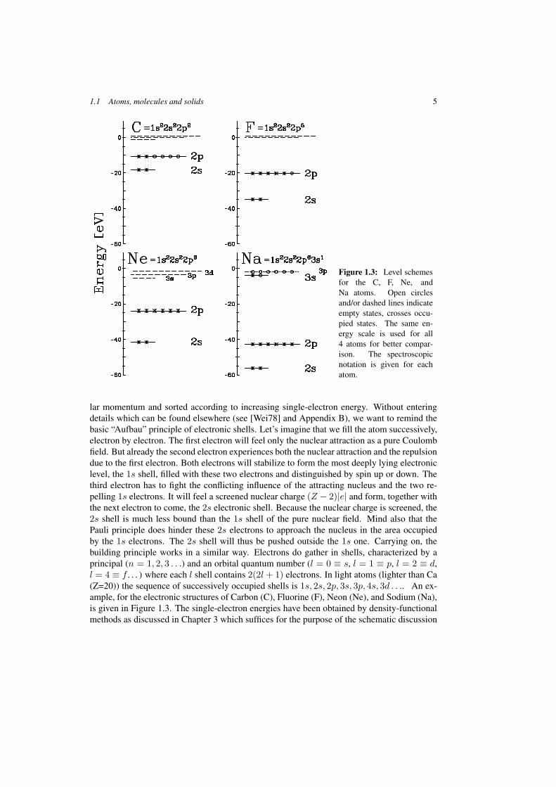
Figure 1.3: Level schemesfor the C, F, Ne, andNa atoms. Open circlesand/or dashed lines indicateempty states, crosses occu-pied states. The same en-ergy scale is used for all4 atoms for better compar-ison. The spectroscopicnotation is given for eachatom.

lar momentum and sorted according to increasing single-electron energy. Without enteringdetails which can be found elsewhere (see [Wei78] and Appendix B), we want to remind thebasic “Aufbau” principle of electronic shells. Let’s imagine that we fill the atom successively,electron by electron. The first electron will feel only the nuclear attraction as a pure Coulombfield. But already the second electron experiences both the nuclear attraction and the repulsiondue to the first electron. Both electrons will stabilize to form the most deeply lying electroniclevel, the 1s shell, filled with these two electrons and distinguished by spin up or down. Thethird electron has to fight the conflicting influence of the attracting nucleus and the two re-pelling 1s electrons. It will feel a screened nuclear charge (Z − 2)|e| and form, together withthe next electron to come, the 2s electronic shell. Because the nuclear charge is screened, the2s shell is much less bound than the 1s shell of the pure nuclear field. Mind also that thePauli principle does hinder these 2s electrons to approach the nucleus in the area occupiedby the 1s electrons. The 2s shell will thus be pushed outside the 1s one. Carrying on, thebuilding principle works in a similar way. Electrons do gather in shells, characterized by aprincipal (n = 1, 2, 3 . . .) and an orbital quantum number (l = 0 ≡ s, l = 1 ≡ p, l = 2 ≡ d,l = 4 ≡ f . . . ) where each l shell contains 2(2l + 1) electrons. In light atoms (lighter than Ca(Z=20)) the sequence of successively occupied shells is 1s, 2s, 2p, 3s, 3p, 4s, 3d . . .. An ex-ample, for the electronic structures of Carbon (C), Fluorine (F), Neon (Ne), and Sodium (Na),is given in Figure 1.3. The single-electron energies have been obtained by density-functionalmethods as discussed in Chapter 3 which suffices for the purpose of the schematic discussion

6 1 About clusters

here. The lowest level, the 1s shell, lies for all examples so deep that it does not fit into thegiven scale. We track here mainly the evolution of the 2s, 2p and 3s shells in the vicinity ofthe rare gas Ne. The nuclear charge, and thus the electron number, increases from C to Naas Z(C) = 6, Z(F) = 9, Z(Ne) = 10, and Z(Na) = 11. The filling of the shells proceedsaccordingly as indicated in the figure. Next to the element symbol we show also the spec-troscopic notation for the shell filling. It is self-explanatory. The example also allows one tounderstand a widely used naming in molecular physics: one speaks of the highest occupiedmolecular orbital (HOMO) and lowest unoccupied molecular orbital (LUMO). The case isclearest for the rare gas Ne here. The HOMO is the 2p shell and the LUMO the 3s. Theenergy difference, which often dominates excitation properties, is called the HOMO–LUMOgap.

The comparison of the various spectra in Figure 1.3 is enlightening. Indeed, althoughthe atoms are quite close to each other in terms of size, they have very different properties.Compare, e.g., the cases of F and Na in which the HOMO in Na is much more loosely boundthan in F. As we shall see below, this feature is at the origin of the different chemical reactivityof these two atoms. The energy difference between occupied and empty states also variessignificantly from one element to the other. In all cases the empty states are only bound bya few eV at most, while the binding energy of the HOMO may vary between about 5 and20 eV. Such differences in the spectra imply differences in the capability of electrons to beremoved from an occupied to an empty state. In other words, not only binding properties ofan assembly of atoms, but for example their response to a laser will significantly vary fromone atom to the other. We shall see examples of such differences at various places below.Furthermore, we shall see that these four atoms exemplify the basic bonding types. And theyhave been used extensively in cluster studies (except maybe for the fact that the preferred raregas for building clusters is Ar rather than Ne).

Going to heavier and heavier atoms the filling of electrons in shells becomes more andmore involved. Nevertheless there exist the so called Hund’s rules as reasonably robust guide-lines for an estimate of the sequence of occupied levels, and of their degree of occupancy. Thefirst rule states that electrons successively occupy the levels 1s, 2s, 2p, 3s, 3p, 4s, 3d, 4p, 5s,4d, 5p, 6s . . . . The rule is strictly correct as long as no d states are involved. As soon as dstates enter the game, the actual electronic structures do not exactly match the filling of theshells monotonously but tend to oscillate between d and s while stepping up the elements.This first rule does not yet predict the electronic structure fully. An open question concernsdegenerate levels. For example, in carbon, the occupied levels are indeed 1s, 2s, and 2p withthe corresponding electronic structure 1s22s22p2. But the 2p state is 2×3-fold degenerate(2px, 2py, 2pz times spin) and the above electronic structure allows 2 out of 6, i.e. 15, equiv-alent choices. The second Hund’s rule states that electrons occupy all degenerate subshellsonce before occupying any level twice. This nevertheless does not yet tell with which spinconfiguration this “democratic” filling is performed. This last open point is addressed by thethird rule which states that the ground state configuration of an atom is the one with maximumnet spin (namely aligned spins). There is a subtle detail to be observed, though, when applyingthe third rule. One has to count electron spins up to half filling and switch to hole spin for theupper half towards the next rare gas. All in all, Hund’s rules, although with some exceptions,provide a useful guideline for predicting the electronic structure and the level filling in anatom. They are especially pertinent in small atoms.

1.1 Atoms, molecules and solids 7

The heavier the atom, the more shells are filled with electrons. However the simple sys-tematic filling of a given sequence of levels is no more ensured in these heavy atoms and fromone element to the next one may observe fluctuations in the filling. This is typically the casein the vicinity of the noble metals such as Ag, Au or Pt. For example, the last occupied shellsof Ag (having Z = 47) are successively 4d with 10 electrons and 5s with one electron. On thebasis of light atoms one would have expected a full s shell (5s2) more bound than an open dshell (4d9). This change is caused by small rearrangements of the mean field which influencethe relative energy of 4d and 5s shells. The bigger surprise rather comes when looking atthe whole sequence: Mo (Z = 42, 4d55s), Tc (Z = 43, 4d55s2), Ru (Z = 44, 4d75s), Rh(Z = 45, 4d85s), Pd (Z = 46, 4d10), Ag (Z = 47, 4d105s). The 5s shell is alternativelyfilled or emptied depending on minimal energetic changes. Not surprisingly, in these caseswhere the two shells, 4d and 5s, are energetically so close, the 4d and 5s electrons are likelyto simultaneously play a role in low energy phenomena. The simplified discussion which weuse here thus becomes insufficient for heavier elements. One needs to think of the spin-orbitsplitting which can easily span the few eV energy differences discussed in the filling of tran-sitional elements. The spin-orbit force is also crucial for the magnetic properties which alsoshow their most dramatic consequences for transitional elements, particularly Fe, Ca, and Ni.

1.1.1.2 The atomic many-body problem

It is obvious from the above qualitative discussion that there is no trivial model to understandthe details of the filling of electron shells. The problem is complex and of many-body nature.The atomic nucleus provides an attractive potential. The quantum mechanics of that is wellknown as it constitutes a central field problem for one electron. The difficulty comes fromthe electron–electron interactions for several electrons simultaneously. Qualitatively, and tosome extent quantitatively, this many body nature of the problem manifests itself in termsof screening. In other words, one electron essentially feels the nuclear field screened by theelectrons belonging to the more bound shells. But the balance is more delicate. First, asalready mentioned, one has to account for the Pauli principle which repels outer electronsfrom the central part of the atom. This exclusion effect still preserves the sphericity of theproblem. More delicate is the fact that electrons belonging to the same shell also repel eachother via the Coulomb interaction. And such an effect has to be accounted for on a one toone basis. Stated so crudely, the problem might appear as awfully complicated. It is indeed,if one looks for spectroscopic details. Global features, however, are more forgiving. Thekey mechanism of simplification lies here in the presence of the external field provided bythe nucleus. Indeed, in spite of the electron–electron corrections, this central attracting fieldsomewhat shapes the gross structure of the electronic spectrum and basically sets a hierarchyin the way one accounts for electron–electron effects. To an acceptable approximation, thesimple screening picture can thus be recast into a self consistent mean field approach in whicheach electron feels an average potential field created by the nucleus and the electron–electroninteractions (including both intra and inter-shell interactions). This is the spirit of the so called“central field” approximation. Let us briefly explain what lies behind this concept.

8 1 About clusters

We start from the many body electron Hamiltonian for an atom with N electrons (posi-tions ri) bound to a nucleus of charge Z

H =N∑i

(− �2

2me∇2

i −Ze2

ri) +

N∑i<j

e2

|ri − rj | (1.1)

where me is the electronic mass (note that we are using the Gaussian system of units, seeAppendix A.1). The central field approximation of Hartree and Slater [Har27, Sla51] is basedon an independent particle picture. One admits that electrons do move in an effective potentialrepresenting the nuclear attraction together with the repulsive interactions with the remainingN − 1 other electrons. As discussed above, the major effects of these N − 1 electrons is toscreen the nuclear charge. Thus the inter-electron repulsive term contains a large sphericallysymmetric component which we shall write as

∑i UH(ri). This means that we can approxi-

mate the effective potential field felt by one electron by a spherically symmetric potential

Utotal(r) = −Ze2/r + UH(r) . (1.2)

The actual form of UH(r) remains to be specified. The asymptotic behaviors can be easilyfixed by requiring recovery of the nuclear field at short distance and of the net charge felt bythe last electron at large distance, namely

Utotal(r) −→r → 0

−Ze2

r, Utotal(r) −→

r → ∞−(Z − N + 1)e2

r. (1.3)

The determination of the effective potential at intermediate range is of course more in-volved as it requires one to account for all the electrons. Many methods have been developedto attack this problem. Let us cite the most famous Thomas-Fermi and Hartree-Fock meth-ods, which both provide a well defined way to compute a central field, actually a mean-fieldpotential common to all the electrons constituting the system (for a detailed discussion andreferences see Chapter 3). The central field approximation turns the initial three dimensional(3D) problem into an effective spherical 1D problem, which can fairly easily be solved withstandard techniques of basic quantum mechanics. The N -electron wavefunction is factorizedinto N one-electron wavefunctions, which in turn can be factorized into a radial and an an-gular part ϕnlm(r) = Rnl(r)Ylm(θ, φ) (with obvious notations). The resolution of the radialSchrodinger equation provides the Rnl(r) and the corresponding principal (n = 1, 2, 3 . . .)and orbital (l = 0, 1, 2 . . .) quantum numbers. There is one subtle feedback loop in that treat-ment: the effective central field is composed from the Coulomb force of actual electron den-sities; these, in turn, depend on the central field. The problem is then resolved by iterating thesolution with subsequent update of the central field until the feedback loop has converged. Af-ter all one disposes of the sequence of one-electron energies in levels 1s, 2s, 2p, 3s, 3p, 4s . . .,as already discussed above. Of course the details of the level filling may vary from one atomto the next, an effect which is related to the actual form of the central field Utotal(r) andits self-consistent arrangement. Such mean field models are widely used in atomic physicsand provide a sound starting basis for more elaborate approaches, taking better into accountcorrelations between electrons. The density functional theory in which these correlations are

1.1 Atoms, molecules and solids 9

expressed in terms of the local electronic density (see Section 3.3.3) offers here a robust start-ing point for such investigations. A first example of applications of this method was given inFigure 1.3 showing the spectra of the four simple atoms C, F, Ne, and Na.

A comment is in order here concerning the meaning of single electron energies, and inparticular its relation to experimental observables. When an atom is excited, for example by alaser, an electron may be promoted from one state of initial energy ε1 to another of energy ε2

(the latter being possibly unbound). Experimentally, one only can access the transition energyε2 − ε1, for example through a photon. This provides the well known series of transitionlines observed in various atoms. But one has to keep in mind that this electronic transition isa complex dynamical process which affects not only the “promoted” electron but the wholeatom. Indeed, the energy levels of an atom with an empty electronic slot (called a hole, h) atlevel ε1 and an (originally empty but now) occupied level ε2 (called a particle, p) are differentfrom the energy levels of the original atom (0ph). All the electrons in the excited (1ph) atomhave to rearrange themselves to account for the electronic modification, and the energy levelsdo the same. This means in particular that, if the excited atom remains bound, the final energyof the “promoted” electron will not exactly be ε2. As a consequence observing the transitionenergy gives a direct access neither to ε1 nor to ε2 of the original atom but includes correctionsfrom a complex (specific) rearrangement process. An ideally instantaneous “promotion” of theelectron (if possible) might leave the rest of the atom frozen and thus indeed give informationon the actual energies of occupied levels in the original atom. In the other extreme case ofan infinitely slow electronic excitation all other electrons do rearrange continuously and onewill rather measure the energies of the final excited atom. The actual experimental situationusually lies in between these two extremes. We shall discuss similar examples in the case ofclusters, see e.g. Sections 2.3.2 and 2.3.8. It is however to be noted that rearrangement effectsare much larger in clusters than they are in atoms, because of possible ionic effects.

1.1.2 Molecules

1.1.2.1 The Mendeleev classification of elements

The successive filling of electronic shells provides the microscopic basis for the understand-ing of chemical properties of elements. Indeed, the early Mendeleev classification, althoughinitially founded on mass rather than on electron number, was precisely trying to explain theregularity observed in the chemical reactivity of apparently different atoms. Since then wehave learned that these chemical similarities reflect the behavior of the tiny fraction of leastbound electrons in atoms, the so called valence electrons. And as long as valence electronsbelong to shells with the same angular momenta (s, p, d . . . shells) the corresponding atomsbehave similarly at the chemical level. This is, after all, not so surprising. The value of theangular momentum of the shell fixes the shape of the electronic wavefunctions and hence thecapability of a given electron of a given atom to interact, and possibly bind, with electrons ofanother atom. The degree of filling also fixes the capability of an atom to accept or to releasevalence electrons. The atoms with completed shells (shell closure) are especially stable. Theso called rare gases (He (Z = 2), Ne (Z = 10), Ar (Z = 18), Kr (Z = 36), Xe (Z = 54),and Rn (Z = 86)) form the family of the most stable atoms. They have the highest values ofionization potential. This explains why these species are particularly inert from the chemical

10 1 About clusters

point of view. In the “vicinity” of these rare gases lie two categories of atoms either with oneelectron more or one electron less than the corresponding rare gas. In turn, these two familiesof atoms are extremely active from the chemical point of view because the atoms belongingto these families have a strong tendency either to grab or to release an electron, in order toattain an electronic configuration similar to that of the neighbor rare gas. The alkaline atoms(Li (Z = 3), Na (Z = 11), K (Z = 19), Rb (Z = 37), Cs (Z = 55), Fr (Z = 87)) have onevalence electron belonging to a s shell as compared to the neighbor rare gas. This s electronis weakly bound, which implies a small ionization potential. Correlatively, it has a strongtendency to leave its parent atom, as we shall see below. On the contrary, the halogen atoms(F (Z = 9), Cl (Z = 17), Br (Z = 35), I (Z = 53), At (Z = 85)) exhibit a valence p shellmissing one electron for closure. They thus have a strong tendency to find this electron in theirsurrounding. Obviously alkaline and halogen atoms are likely to “complement” each other.An alkaline atom will tend to “give” its peripheral s electron to a halogen atom to complete itsp shell. This exchange of electrons forms the basis of the most robust chemical bond, the ionicbond in which electron exchange ensures a robust electrostatic binding between two chargedspecies, a positively charged alkaline and a negatively charged halogen. We shall come back tothis below. But before exploring more systematically binding possibilities between atoms, onehas first to come back to the Mendeleev classification for a few more remarks. Up to now wehave discussed only 3 columns of atoms (rare gas, alkalines, halogens) while the Mendeleevclassification contains up to 18 columns. In fact, halogens and alkalines, as “ends” of eachrow do represent the extremes cases of tendencies which develop along each row of the clas-sification. Starting from an alkaline atom, successively adding electrons (namely going in thedirection of the next heavier halogen) will progressively attenuate the tendency of the atomto release electrons and increase its tendency to grab them. There is thus a continuous pathbetween electron donors and electron acceptors. In the middle of the path lie atoms with an“equal” tendency to grasp or to release electrons. The typical representatives of this class arecarbon (C, Z = 6) silicon (Si, Z = 14) and germanium (Ge, Z = 32). We shall see that theytend to bind between each other in a specific way giving rise to a very rich palette of molecularstructures, particularly for carbon.

1.1.2.2 A pedestrian view of bonding

The first step along the path from atoms to molecules (and to clusters) is represented by dimermolecules and we shall here focus on this simple case. As already mentioned, depending ontheir electronic structures two atoms may, or may not, bind together, with different type andstrength of binding. Chemical binding is by nature a low energy phenomenon, involving atmost a few eV energy. For this reason only valence electrons significantly play a role, andthe Mendeleev classification thus provides a gross map of which atom may possibly bind withwhich other and how. Of course, binding between two atoms is a matter of electrons andenergy. The key question is thus whether the valence electron(s) of a given atom may find itenergetically interesting to “leave” their parent atom to “bind” to another atom, or whetherthere are “intermediate” solutions for these electrons, like partial attachment to both atoms.According to such a simple picture, one may envision four classes of binding reflecting thepossibility of sharing the set of valence electrons between the two partner atoms, as illustratedin Figure 1.4. As in any scheme, these bonding types are idealized extremes. Real moleculesare usually dominated by one of these bondings with admixtures of the complementing types.

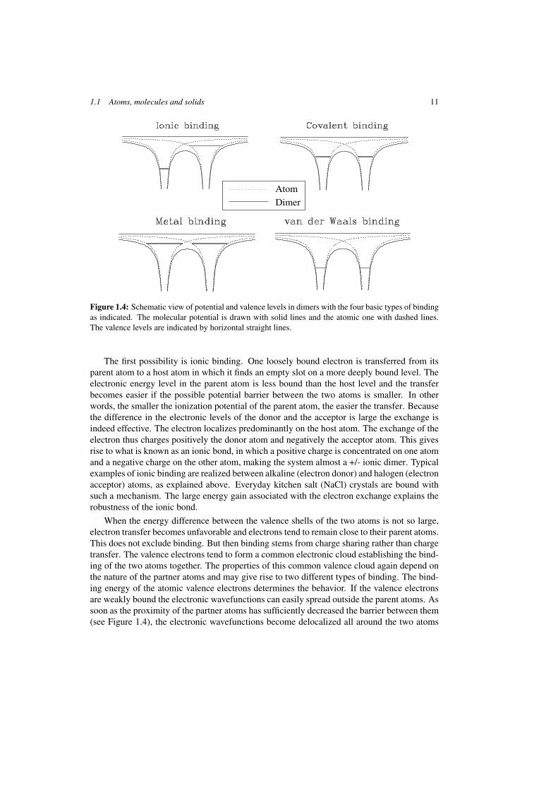
1.1 Atoms, molecules and solids 11

AtomDimer

Figure 1.4: Schematic view of potential and valence levels in dimers with the four basic types of bindingas indicated. The molecular potential is drawn with solid lines and the atomic one with dashed lines.The valence levels are indicated by horizontal straight lines.

The first possibility is ionic binding. One loosely bound electron is transferred from itsparent atom to a host atom in which it finds an empty slot on a more deeply bound level. Theelectronic energy level in the parent atom is less bound than the host level and the transferbecomes easier if the possible potential barrier between the two atoms is smaller. In otherwords, the smaller the ionization potential of the parent atom, the easier the transfer. Becausethe difference in the electronic levels of the donor and the acceptor is large the exchange isindeed effective. The electron localizes predominantly on the host atom. The exchange of theelectron thus charges positively the donor atom and negatively the acceptor atom. This givesrise to what is known as an ionic bond, in which a positive charge is concentrated on one atomand a negative charge on the other atom, making the system almost a +/- ionic dimer. Typicalexamples of ionic binding are realized between alkaline (electron donor) and halogen (electronacceptor) atoms, as explained above. Everyday kitchen salt (NaCl) crystals are bound withsuch a mechanism. The large energy gain associated with the electron exchange explains therobustness of the ionic bond.

When the energy difference between the valence shells of the two atoms is not so large,electron transfer becomes unfavorable and electrons tend to remain close to their parent atoms.This does not exclude binding. But then binding stems from charge sharing rather than chargetransfer. The valence electrons tend to form a common electronic cloud establishing the bind-ing of the two atoms together. The properties of this common valence cloud again depend onthe nature of the partner atoms and may give rise to two different types of binding. The bind-ing energy of the atomic valence electrons determines the behavior. If the valence electronsare weakly bound the electronic wavefunctions can easily spread outside the parent atoms. Assoon as the proximity of the partner atoms has sufficiently decreased the barrier between them(see Figure 1.4), the electronic wavefunctions become delocalized all around the two atoms

12 1 About clusters

and one then speaks of a metallic bond (as a precursor of the behavior of such systems in thebulk, discussed below). Alkalines are the typical elements which establish metallic bonds be-tween each other. They are called simple metals because of the well separated valence electron(see Na in Figure 1.3). We shall often consider the generic example of Nan clusters as typicalsimple metallic systems. Metallic binding is also observed in more complicated metals suchas, e.g., Cu, Ag, Au, or Pt. The valence binding mechanism in these systems is qualitativelysimilar to the simple case of alkalines, but there is then a d shell energetically close to thevalence s shell (see the example of Cu in Figure 3.2). This causes strong polarization effectswith impact on binding and other dynamical properties (see e.g. the discussion of opticalresponse in Section 4.3.4.1).

The metallic binding does not exhaust all possibilities of sharing a common valence cloud.If the electrons are initially more strongly bound to their parent atom, electron delocalizationcannot fully develop and electrons gather in the region of smallest potential energy, betweenthe two partner atoms. One then speaks of a covalent bond. The typical covalent bond isrealized between atoms like C or Si in which atomic valence electrons are fairly well bound(see also Figure 1.3). However, one has to keep in mind that covalent and metallic bonds areidealized situations. There is a smooth transition between these extremes. It is usually hardto disentangle these two types in small molecules. The distinction becomes better defined inbulk material where interstitial density and conductivity add useful criteria [AM76].

When valence electrons are too deeply bound in the atom, neither charge transfer norcharge sharing are possible between the two atoms. Because the HOMO electrons are toodeeply bound, the electrons cannot escape the attraction of their parent atom. One may thenwonder how bonding is possible at all. Although electrons remain localized around theirparent atom, the electronic cloud of each atom is influenced by the partner atom. This virtualpolarization of the electronic clouds results in mutual dipole-dipole interactions between thetwo atoms, which establishes a binding of the system. As is obvious the resulting bond ismuch weaker than the previous ionic, metallic or covalent bonds. And yet, it suffices forthe binding of rare gas molecules up to possibly large compounds, as we shall see below.This type of loose binding is known as van der Waals (or molecular) binding, in referenceto the interactions between two neutral atoms or molecules. The typical cases of van derWaals bonding thus concern rare gas atoms mostly. It should be noted that the details of thebinding mechanism are somewhat involved. The polarization of the electronic cloud has to beunderstood as a dynamical correlation effect, with constantly fluctuating dipoles, rather than asa mere static polarization. To properly account for this effect requires a quantum mechanicaltreatment which we shall not discuss here.

All in all, simple energetic considerations for the HOMO, as exemplified in Figure 1.3, al-low one to identify four major types of bonding between atoms, as schematically representedin Figure 1.4. These energetic aspects reflect themselves in the degree of localization of theelectrons binding the two atoms: the more bound the electrons, the more localized their wave-functions. Of course, just like the behavior of atoms as electron donors or acceptors, there isno clear separation between the various binding mechanisms, but rather a continuous path be-tween them (see Figure 1.8 for an example in the bulk). Still, the four classes identified abovecan be seen as robust guidelines for understanding the binding of most molecular systems.Finally, it should be noted that one sometimes introduces a few other classes of binding. Theterm “molecular binding” for example refers to the binding between molecules, while the term

1.1 Atoms, molecules and solids 13

“van der Waals” usually concerns atoms, although in both cases the basic binding mechanismis the same. Similarly one sometimes speaks of “hydrogen bonding” to label covalent bindinginvolving hydrogen atoms. Because its particularly large ionization potential, hydrogen usu-ally establishes especially robust bonds (as compared to standard covalent bonds) with otherspecies, hence the specific label. Again, such fine distinctions do not basically alter our globalclassification scheme. We shall thus ignore such details in the following.

1.1.2.3 Deeper into microscopic mechanisms

Before proceeding to the bulk (in Section 1.1.3) and to clusters (in Section 1.2) we would liketo discuss in some more detail the binding mechanism for simple dimers, in order to exhibitthe dominant mechanisms in a semi-quantitative fashion. We keep the discussion at a minimallevel of formalism. More detailed elaborations of that sort can be found in many standardtextbooks on molecular physics or chemistry (see Appendix A.4).

We consider the case of a dimer formed from two atoms A and B, each having one svalence electron (as is the case for H or Na). The atoms are placed at a distance R fromeach other. We denote by ϕA and ϕB the respective atomic single-electron wavefunctionsfollowing the Schrodinger equations

− �2

2m∆ϕX + VXϕX = εXϕX , X ∈ {A, B} , (1.4)

where VX labels the potential felt by the valence electron in atom X and εX is the correspond-ing eigenvalue of energy. In order to simplify the problem further, we restrict ourselves to thecase of an ionized dimer, in which only one active electron is left (as in H+

2 or Na+2 ). The goal

is then to solve the Schrodinger equation for the dimer electron

− �2

2m∆ϕAB + VABϕAB = εABϕAB , (1.5)

where εAB labels the energy of the electron level binding the dimer. The total potential VAB

is, in principle, a self consistent quantity as it depends on the wavefunction ϕAB itself, becausethe formation of the bond induces an electronic rearrangement and thus a modification of thenet atomic fields. For the sake of simplicity and because these rearrangement effects can beassumed reasonably weak, at least for an exploratory approach, we approximate VAB by

VAB � VA + VB +e2

R. (1.6)

For the solution we assume that we can represent the molecular electronic wave function ϕAB

in terms of the given atomic wave functions. This means that we make the ansatz of LinearCombination of Atomic Orbitals (LCAO)

ϕAB = cAϕA + cBϕB . (1.7)

It remains to determine the expansion coefficients cA and cB .

14 1 About clusters

Variation of the total energy with respect to these coefficients yields in a straightforwardmanner the secular equation(

εA + e2

R (ε + e2

R )S + h

(ε + e2

R )S + h εB + e2

R

)(cA

cB

)= εAB

(1 SS 1

)(cA

cB

)(1.8)

where

S =∫

drϕ∗AϕB , h =

∫drϕ∗

AV ϕB ,

εA = εA +∫

drϕ∗AVBϕA , εB = εB +

∫drϕ∗

BVAϕB ,

ε =εA + εB

2, V =

VA + VB

2.

The key quantities for the mixing are the overlap (S) and bond (h) integrals. They providemeasures of how much the two electronic wavefunctions “communicate”, either “directly”(overlap integral) or via the interaction (bond integral). In the limit of a sufficiently smalloverlap integral S the two solutions ε+,−

AB of the secular equation Eq. (1.8) take the simpleforms (∆ε = εA − εB)

ε±AB = ε + |h|S ∓√

h2 + ∆ε2/4 (1.9)

where the most bound level ε+AB is known as the bonding state while the least bound one

ε−AB is the antibonding state. Both the bond and the overlap integrals enter the expressionsof ε±AB . Because by construction the bond integral is less than 1, the bonding state is alwaysmore bound than the most bound atomic level εAB ≤ min(εA, εB) (note that the cross-overelements are negative, e.g.

∫drϕ∗

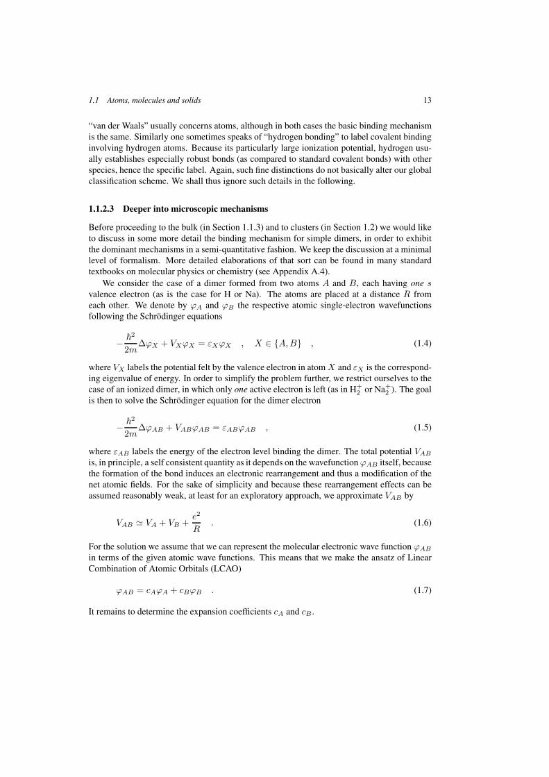
AVBϕA < 0), which is what establishes binding. The netgain of binding then depends on S and h, which points out the importance of the capabilityof electrons to explore the partner atom (S and h). Note finally that the energy separationbetween bonding and antibonding states increases with the bond integral. These behaviorsare illustrated for the case of homonuclear dimers in the schematic Figure 1.5. Note thathere εA = εB and thus ∆ε = 0. The lower part shows how the matrix elements S and |h|decrease quickly as a function of molecular distance R. Similarly behaves the convergenceε±AB −→ ε = εA = εB for large R.

The energetic information provided by Eq. (1.9) can be nicely complemented by lookingat the spatial extension of the electronic cloud. The interesting quantity is here the electronicdensity ρ+

AB(r) = |ϕ+AB(r)|2 of the bonding state. It reads

ρ+AB(r) = (1 + αi)ρA(r) + (1 − αi)ρB(r) + αcρbond(r) , (1.10a)

ρbond = 2ϕ∗AϕB − S(ρA + ρB) , (1.10b)

ρX = ϕ∗XϕX for X ∈ {A, B} , (1.10c)

αc =[1 +

∆ε

2|h|]−1/2

, αi =∆ε

2|h|αc . (1.10d)

The relations simplify in the homonuclear case, where ∆ε = 0, to αc = 1, αi = 0 and finallyto ρ−AB = ρA + ρB + ρbond. It shows that the bond density makes all the difference.

1.1 Atoms, molecules and solids 15

Figure 1.5: Schematic plot of the over-lap (S) and bond (h) integrals (bottompart) and of the energies of the bonding(ε+

AB) and antibonding (ε−AB) levels as afunction of distance R between the twoatoms. Scales are arbitrary, but note thatthe overlap integral tends towards 1, atshort R. Asymptotically (large R) bothS and h integrals vanish and ε±AB → ε,namely the dimer becomes a collection oftwo independent atoms. The dip in (ε+

AB)at finite distance corresponds to the bondlength, namely the equilibrium distance db

between the two bound atoms forming adimer. The difference between ε±AB(db)and εA (or εB) represents the dissociationenergy of the dimer.

Let us briefly discuss the case of a heteronuclear system (A = B) which is already pre-pared in the above equations. The difference ∆ε � εA − εB shows up at the level of thebonding and antibonding energies. Note that the energy of the bonding state, and thus thenature of binding also depend on the energy difference between the two original atomic or-bitals. It also sensitively enters the total electronic density ρAB(r) given in Eq. (1.10). Thenow non-trivial parameter αi provides a measure of the ionic charge renormalization, henceof the amount of electron density transferred from one atom to the other. Obviously the mostcovalent bond corresponds to αi = 0, as is the case in a homonuclear system. Otherwise, ifαi > 0 (εA ≤ εB), the electron density gathers around A as in a more or less ionic bond.All in all, the two parameters αi, αc thus provide a measure of the degree of ionicity of thebond, allowing one to span in a continuous way the various situations between pure covalent(αi = 0, αc = 1) and pure ionic (αi = 1, αc = 0) binding.

1.1.2.4 More realistic examples

For sake of simplicity, we have restricted our discussion, up to now, to the case of ionizeddimers, with only one active valence electron. Passing to neutral dimers is qualitatively easyto grasp, but computationally more involved. As soon as two electrons, one from each atom,bind together, one has to take into account the Coulomb repulsion between the two electrons.It affects both the energies ε±AB and the repartition of the electronic density ρAB(r). Nonethe-less, the above discussions remain qualitatively valid, in particular concerning the roles ofthe parameters governing the basic properties of the bond (bond and overlap integrals, energydifference ∆ε). To obtain quantitative results in practice, an explicit and detailed calculationof electronic structure has to be performed, starting from a microscopic description of eachatom, usually including more than only valence electrons. And it will turn out that the detailsof electronic spectra (both occupied and empty states) are actually to be accounted for. Wewill address these theoretical methods in Chapter 3.

16 1 About clusters

type v. d. Waals metallic covalent ionic

example Ar2 Na2 C2 NaF

D [eV] 0.010 0.74 6.2 5.0

db [a0] 7.1 5.8 2.3 3.5

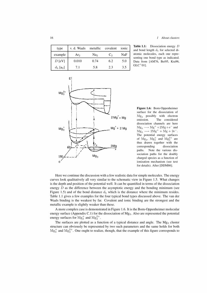
Table 1.1: Dissociation energy Dand bond length db for selected di-atomic molecules, each one repre-senting one bond type as indicated.Data from [AM76, Bei95, Kra96,GLC+01].

Mg32+

Mg3+

Mg3

Mg++ Mg2

Mg+

+ 2 Mg

3Mgre2+ re

+ re

θ

E

Figure 1.6: Born-Oppenheimersurface for the dissociation ofMg3 possibly with electronemission. The considereddissociation channels are hereMg3 −→ Mg+ +2Mg+e− andMg3 −→ 2Mg+ + Mg + 2e−.The potential energy surfacesof Mg3, Mg+

3 and Mg2+3 are

thus drawn together with thecorresponding dissociationpaths. Note the various dis-sociation paths for the doublycharged species as a function ofionization mechanism (see textfor details). After [DDM86].

Here we continue the discussion with a few realistic data for simple molecules. The energycurves look qualitatively all very similar to the schematic view in Figure 1.5. What changesis the depth and position of the potential well. It can be quantified in terms of the dissociationenergy D as the difference between the asymptotic energy and the bonding minimum (seeFigure 1.5) and of the bond distance db which is the distance where the minimum resides.Table 1.1 gives a few examples for the four typical bond types discussed above. The van derWaals binding is the weakest by far. Covalent and ionic binding are the strongest and themetallic example is slightly weaker than these.

A more complex case is demonstrated in Figure 1.6. It is the Born-Oppenheimer molecularenergy surface (Appendix C.1) for the dissociation of Mg3. Also are represented the potentialenergy surfaces for Mg+

3 and Mg2+3 .

The surfaces are plotted as a function of a typical distance and angle. The Mg3 clusterstructure can obviously be represented by two such parameters and the same holds for bothMg+

3 and Mg2+3 . One ought to realize, though, that the example of this figure corresponds to

1.1 Atoms, molecules and solids 17

a particularly simple case, because of the small size of the system. A complex molecule (orcluster) has many ionic degrees of freedom. The molecular energies thus correspond to hugemulti-dimensional Born-Oppenheimer surfaces from which one can inspect at most well takencuts. Such large systems are treated in practice by more direct dynamical methods as will beoutlined in Chapter 3.

Several dissociation channels are sketched in Figure 1.6, depending on the degree of ion-ization (singly or doubly charged Mg3). As can be seen from the figure the correspondingpotential energy surfaces do differ in shape. For example one sees that the more charged thecluster, the more compact the ground state configuration, corresponding to the minimum ofthe potential well. The figure also demonstrates the various possible dissociation paths as afunction of the excitation process. When the cluster is only singly charged it still corresponds,not surprisingly, to a well stable species. When it is doubly charged the picture becomesmore involved. Indeed, if electron removal is sequential, the system, having lost one electron,may have time to relax towards the corresponding equilibrium Mg+

3 state, before a secondionization promotes it, again, towards an equilibrium (although very weakly bound, and thusprobably metastable) state, this time for Mg2+

3 . On the contrary, in the case of a simultane-ous double ionization the system is immediately promoted towards an unstable configurationwhich directly dissociates. We find here an illustration, in the case of a small cluster, of theimportance of the details of the dynamics in the ionization process. We shall come back tothis question at many places (see for example Sections 2.3.2 and 2.3.8).

1.1.3 The point of view of solid state physics

Complementing the discussion on atom and molecule, we now turn to bulk matter. Bulk mighthave two different meanings in the case of clusters. Clusters are often in a liquid state, becauseof their high formation temperature (Section 2.1.3.1). When extrapolating, bulk then refers toa macroscopic liquid. But the ground state (low temperature state) of a cluster stays in a frozengeometry, and bulk then refers to an infinite solid, more precisely a crystal. In the followingdiscussion we shall only consider this zero temperature situation and bulk will thus mean apiece of solid material.

From the viewing angle of solid state physics, a key parameter of classification is theconductivity of a given piece of material. One will thus separate solids into two classes:conductors and insulators. The different bonding types will be associated to these two classes.We shall first, as in the case of atoms/molecules, consider the problem at a qualitative level,before addressing the question from a more formal point of view.

1.1.3.1 Bond types in solids

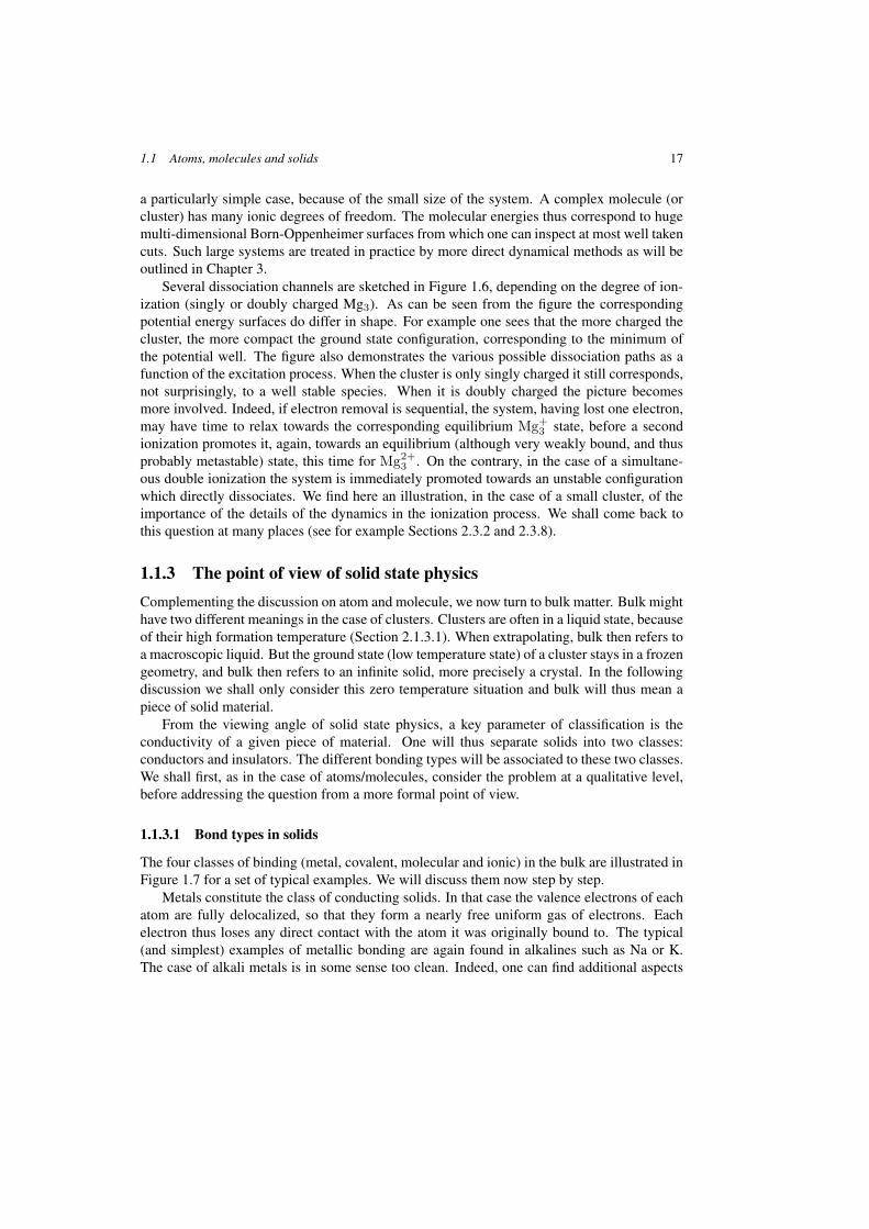
The four classes of binding (metal, covalent, molecular and ionic) in the bulk are illustrated inFigure 1.7 for a set of typical examples. We will discuss them now step by step.

Metals constitute the class of conducting solids. In that case the valence electrons of eachatom are fully delocalized, so that they form a nearly free uniform gas of electrons. Eachelectron thus loses any direct contact with the atom it was originally bound to. The typical(and simplest) examples of metallic bonding are again found in alkalines such as Na or K.The case of alkali metals is in some sense too clean. Indeed, one can find additional aspects

18 1 About clusters

(c) covalent

(b) ionic(a) Van der Waals

(d) metallic

Figure 1.7: Schematic representation of electronic charge distributions in examples of solids. The small(filled) circles represent the ionic cores, with the corresponding “effective” charges seen by the electronsconstituting the binding. The shaded areas represent regions in which one finds an appreciable amountof the electron density. Note that the electronic density is not uniform. The four cases correspond to thebasic four types of binding: a) van-der-Waals (molecular) binding in an Ar crystal, b) ionic binding inKCl, c) covalent binding in C and d) metallic binding in K. After [AM76].

of van der Waals or covalent bonding in many metals, particularly in noble metals whereloosely bound d electrons participate in the bonding. A typical example is Ag, in which theleast bound electron belongs to a 5s shell, while the loosely bound 4d orbitals are stronglydistorted by the presence of neighbor atoms. In such a case the separation between valenceand core electrons is much less clear than in alkalines. And yet, such materials do also exhibita clearly metallic behavior.

Materials with a poor conductivity belong to the category of insulators. But contrarilyto the class of metals, bonding in insulators covers different forms, essentially reflecting thedegree of localization of electrons around their parent atom. Let us successively considerthese various bindings as a function of the degree of localization of electrons, while keepingin mind that the largest degree of delocalization is attained in metals.

In covalent crystals, one faces a set of semi-localized electrons, which gather along thelines joining atoms together. The typical example of such a binding is the case of diamond.Just as in simple molecules, we find a covalent nature of binding in carbon based materials.

The last two classes of insulators leave electrons fully localized on atomic sites. In van-der-Waals crystals such as solid noble gas (e.g., Ne, Ar, Kr, or Xe), very few electrons gatherbetween the sites. Electrons basically remain bound to the original atom they were attachedto. Just as in simple molecules, polarization effects are responsible for the binding of thesystem. The last class of compounds are ionic crystals which associate metallic (electrondonor) and non-metallic (electron acceptor) atoms in a regular manner, so that ionic bonds

1.1 Atoms, molecules and solids 19

(see Section 1.1.2.2) can be reconstituted. In that case electrons are highly localized on atomicsites, once they have been transferred from the metal to the non-metal atoms. The typicalexample of such systems are alkaline halogen compounds such as NaCl, NaF, or LiF.

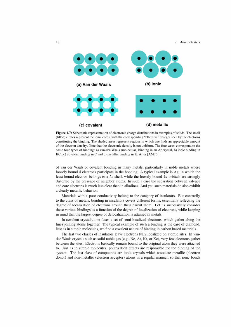
Figure 1.8: Schematic representation of the path between a perfectly covalent and a perfectly ioniccrystal. a) Perfectly covalent Ge crystal: in this case 4 electrons are identically distributed about theGe4+ cores; the electronic density is large along the interstitial directions; b) Covalent GaAs crystal:again density along the interstitial directions, but the electrons gather more around As5+ than aroundGa3+, which gives a slightly ionic character to the system. c) Even more ionic CaSe crystal: the trendof GaAs is even enhanced in that the Ca2+ cores are almost denuded of electrons, to the benefit of theSe6+ cores; still, the crystal keeps a slight covalent character. d) Perfectly covalent ionic KCl crystal:electrons have been fully stripped from the K and transferred to the Cl7+ cores. The electronic structuresof the atoms considered here are: Germanium (Ge, (Ar)3d104S24p2), Gallium (Ga, (Ar)3d104S24p),Arsenic (As, (Ar)3d104S24p3), Selenium (Se, (Ar)3d104S24p4), Calcium (Ca, (Ar)4s2), Chlorine (Cl,(Ne)3s23p5) and Potassium (K, (Ar)4s2). From [AM76].

It is clear from the above brief discussion that the solid state physics classification ofbonding, not surprisingly, matches the classification of molecular physics. The analogies goeven further. It was already discussed for molecules in Section 1.1.2 that the four types ofbonding are idealizations and that reality often resides in between. Figure 1.8 complementsthat for crystals showing the path from covalent to ionic binding. Starting from the covalentGermanium crystal one observes, by associating successively atoms on both (complementing)

20 1 About clusters

sides of Ge, a continuous transition towards the ionic KCl crystal. As we shall see below,clusters provide here an even more interesting option. They allow one to span a continuouspath from atom to bulk. And one finds situations where the nature of bonding changes withsystem size.

1.1.3.2 Band theory in solids

A general theory of bonding in solids can be found in many specialized textbooks [AM76,Pet95]. We give here a brief summary of level structure in solids, and discuss how such a levelstructure is related to the nature of bonding. We start with a simple model crystal in 1D. Theionic lattice introduces an attractive potential U(x) which alters the otherwise free motion ofelectrons and turns out to be responsible for the level structure. Taking a mesh size a, latticeperiodicity implies a specific form for electron orbitals

U(x + na) = U(x) =⇒ ϕk(x + na) = exp(ikna)ϕk(x) (1.11)

where n means any integer and k is the so-called lattice momentum. As is clear from this formof the wavefunction (Bloch ansatz), it is sufficient to consider values of k in the first Brillouinzone defined by −π/a ≤ k ≤ π/a. Other values only repeat phase factors exp(ikna) fromthe first zone.

The problem thus amounts to solving the Schrodinger equation for ϕk in an elementarycell 0 ≤ x ≤ a with the above defined periodic boundary conditions at x = 0 and x = a(Bloch condition). For the sake of simplicity we assume that U(x) is furthermore a squarewell potential of depth U0 and width a− b, so that b also represents the barrier width betweentwo neighboring wells, i.e.

U(x) ={ −U0 for

∣∣ξ − a2

∣∣ ≤ a−b2

0 for∣∣ξ − a

2

∣∣ > a−b2

, ξ = mod (x, a) . (1.12)

Inside the well, as is well known, the wavefunction takes an oscillatory form ϕk(x) =-A exp(iKx) +B exp(−iKx) where K is directly associated to the level energy E as K =√

2mE/�2. Outside the well (or inside the barrier) the wavefunction takes an exponentialform ϕk(x) = A exp(κx) + B exp(−κx) with (κ =

√2m(U0 − E)/�2). The coefficients

A, B, C, D are found by matching ϕk and dϕk/dx at boundaries x = b and x = a and impos-ing the Bloch periodic condition Eq. (1.11) on ϕk. This provides an implicit equation linkingK, κ, k, b and a. For a qualitative discussion, we consider here the simple case of vanish-ingly narrow potential barrier b → 0 and increasing barrier height U0 → ∞ (within imposingconstant U0b). The implicit equation then reduces to the simple form

cos Ka + µsin Ka

Ka= cos ka with µ =

ma

�2U0b (1.13)

The above equation links the electron energy E = �2K2/2m to the so called Bloch vector k.

Bloch-like solutions ϕk therefore exist only for values of K, and hence E, which are solutionsof Eq. (1.13) for a given k. Whatever k may be, the r.h.s. of Eq. (1.13) is bound by ±1. Theallowed values of K, and hence of electronic energies E, thus obey the constraint

| cosKa + µsin Ka

Ka| ≤ 1 . (1.14)

1.1 Atoms, molecules and solids 21

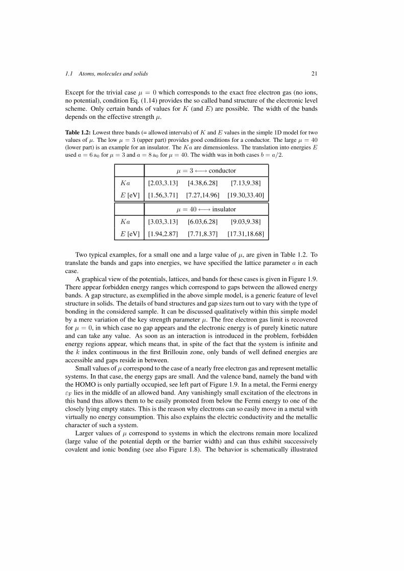
Except for the trivial case µ = 0 which corresponds to the exact free electron gas (no ions,no potential), condition Eq. (1.14) provides the so called band structure of the electronic levelscheme. Only certain bands of values for K (and E) are possible. The width of the bandsdepends on the effective strength µ.

Table 1.2: Lowest three bands (= allowed intervals) of K and E values in the simple 1D model for twovalues of µ. The low µ = 3 (upper part) provides good conditions for a conductor. The large µ = 40(lower part) is an example for an insulator. The Ka are dimensionless. The translation into energies Eused a = 6a0 for µ = 3 and a = 8a0 for µ = 40. The width was in both cases b = a/2.

µ = 3 ←→ conductor

Ka [2.03,3.13] [4.38,6.28] [7.13,9.38]

E [eV] [1.56,3.71] [7.27,14.96] [19.30,33.40]

µ = 40 ←→ insulator

Ka [3.03,3.13] [6.03,6.28] [9.03,9.38]

E [eV] [1.94,2.87] [7.71,8.37] [17.31,18.68]

Two typical examples, for a small one and a large value of µ, are given in Table 1.2. Totranslate the bands and gaps into energies, we have specified the lattice parameter a in eachcase.

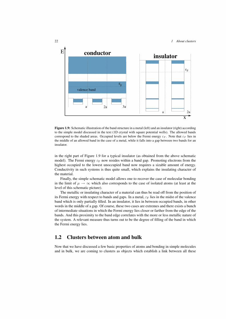
A graphical view of the potentials, lattices, and bands for these cases is given in Figure 1.9.There appear forbidden energy ranges which correspond to gaps between the allowed energybands. A gap structure, as exemplified in the above simple model, is a generic feature of levelstructure in solids. The details of band structures and gap sizes turn out to vary with the type ofbonding in the considered sample. It can be discussed qualitatively within this simple modelby a mere variation of the key strength parameter µ. The free electron gas limit is recoveredfor µ = 0, in which case no gap appears and the electronic energy is of purely kinetic natureand can take any value. As soon as an interaction is introduced in the problem, forbiddenenergy regions appear, which means that, in spite of the fact that the system is infinite andthe k index continuous in the first Brillouin zone, only bands of well defined energies areaccessible and gaps reside in between.

Small values of µ correspond to the case of a nearly free electron gas and represent metallicsystems. In that case, the energy gaps are small. And the valence band, namely the band withthe HOMO is only partially occupied, see left part of Figure 1.9. In a metal, the Fermi energyεF lies in the middle of an allowed band. Any vanishingly small excitation of the electrons inthis band thus allows them to be easily promoted from below the Fermi energy to one of theclosely lying empty states. This is the reason why electrons can so easily move in a metal withvirtually no energy consumption. This also explains the electric conductivity and the metalliccharacter of such a system.

Larger values of µ correspond to systems in which the electrons remain more localized(large value of the potential depth or the barrier width) and can thus exhibit successivelycovalent and ionic bonding (see also Figure 1.8). The behavior is schematically illustrated

22 1 About clusters

�

�E

x

εF

a 2a 3a

valence band

conductor

Fε

a 2a

insulator

Figure 1.9: Schematic illustration of the band structure in a metal (left) and an insulator (right) accordingto the simple model discussed in the text (1D crystal with square potential wells). The allowed bandscorrespond to the shaded areas. Occupied levels are below the Fermi energy εF . Note that εF lies inthe middle of an allowed band in the case of a metal, while it falls into a gap between two bands for aninsulator.

in the right part of Figure 1.9 for a typical insulator (as obtained from the above schematicmodel). The Fermi energy εF now resides within a band gap. Promoting electrons from thehighest occupied to the lowest unoccupied band now requires a sizable amount of energy.Conductivity in such systems is thus quite small, which explains the insulating character ofthe material.

Finally, the simple schematic model allows one to recover the case of molecular bondingin the limit of µ → ∞ which also corresponds to the case of isolated atoms (at least at thelevel of this schematic picture).

The metallic or insulating character of a material can thus be read off from the position ofits Fermi energy with respect to bands and gaps. In a metal, εF lies in the midst of the valenceband which is only partially filled. In an insulator, it lies in between occupied bands, in otherwords in the middle of a gap. Of course, these two cases are extremes and there exists a bunchof intermediate situations in which the Fermi energy lies closer or farther from the edge of thebands. And this proximity to the band edge correlates with the more or less metallic nature ofthe system. A relevant measure thus turns out to be the degree of filling of the band in whichthe Fermi energy lies.

1.2 Clusters between atom and bulk

Now that we have discussed a few basic properties of atoms and bonding in simple moleculesand in bulk, we are coming to clusters as objects which establish a link between all these

1.2 Clusters between atom and bulk 23

cases. We try to work out their specificity and to explain why they are more than just largemolecules or small pieces of bulk.

1.2.1 Clusters as scalable finite objects

Clusters are, by definition, aggregates of atoms or molecules with regular and arbitrarily scal-able repetition of a basic building block. Their size is intermediate between atoms and bulk.One could thus loosely characterize them with a formula of the form Xn (3<∼n<∼105−7). Theactual upper limit in size is hard to fix. As we shall see below, the definition of bulk may varyfrom one observable to another, namely a given physical property may reach its bulk value fora size different from another observable.

1.2.1.1 Clusters are more than molecules

Molecules usually have a well defined composition and structure. Think, e.g., of the wellknown molecules such as C6H6. Such systems have only a small number of isomers, a fewunits at most, even if they are themselves not small molecules. This is different for clusters,which often possess a large number of energetically close isomers and in which the number ofisomers grows huge with increasing cluster size. For example, in such a small cluster as Ar13,one has found hundreds of isomers, the actual number slightly depending on the detail ofthe interatomic potential used in the calculations, while less than 10 isomers were identifiedin Ar8 [DJB87]. Another example are metal clusters which are also swamped by isomers,because of the softness of the binding.

When facing such a huge number of isomers, it is obvious that it is very hard to simplyassess which is the most stable structure. This holds the more so as clusters are formed atfinite temperature where it may be a delicate task to precisely tune the actual temperatureof the formed clusters (see Section 2.1). Such a finite temperature allows a given cluster toexplore a huge variety of isomers (=shapes), by simple thermal activation. And this processis all the more important as the number of accessible isomers is large. Stated in another,more technical, way, the potential energy surface (Born-Oppenheimer surface as discussedin Section 3.4.2) is very flat and this makes it very hard to figure out the actual ground-statestructure of the system. Standard quantum chemistry techniques, well adapted to moleculeswith few isomers, are here often at a loss. Note finally that the difficulty in identifying theactual ground state structure constitutes an example of a more general feature, namely thatmany cluster properties do strongly depend on cluster size, see e.g. the example of shapes inSection 4.1.3.

1.2.1.2 Clusters are more than finite pieces of bulk

There are several features which distinguish a small piece of bulk from bulk [Ber98]. Thebasic difference between bulk and clusters can be seen from the level structure. Finite systemsare basically characterized by discrete levels, at least in the low energy part of their spectrum.As is well known (see also Section 1.1.3.2), single-electron spectra in solids come along inbands each containing a continuum of levels. Passing from a discrete to a continuous set oflevels is, in fact, also a continuous process. We have seen in Section 1.1.2.3 that the binding

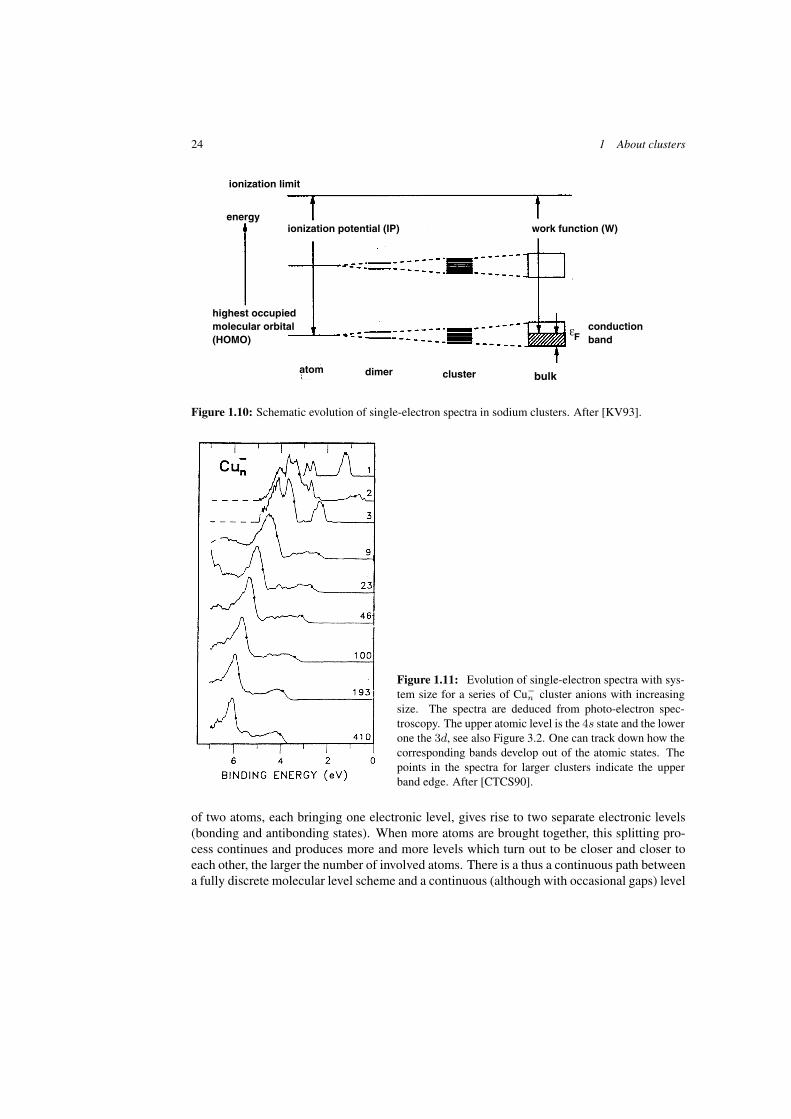
24 1 About clusters

highest occupied molecular orbital(HOMO)

εFconductionband

atom clusterdimer bulk

work function (W)ionization potential (IP)energy

ionization limit

Figure 1.10: Schematic evolution of single-electron spectra in sodium clusters. After [KV93].

Figure 1.11: Evolution of single-electron spectra with sys-tem size for a series of Cu−

n cluster anions with increasingsize. The spectra are deduced from photo-electron spec-troscopy. The upper atomic level is the 4s state and the lowerone the 3d, see also Figure 3.2. One can track down how thecorresponding bands develop out of the atomic states. Thepoints in the spectra for larger clusters indicate the upperband edge. After [CTCS90].

of two atoms, each bringing one electronic level, gives rise to two separate electronic levels(bonding and antibonding states). When more atoms are brought together, this splitting pro-cess continues and produces more and more levels which turn out to be closer and closer toeach other, the larger the number of involved atoms. There is a thus a continuous path betweena fully discrete molecular level scheme and a continuous (although with occasional gaps) level

1.2 Clusters between atom and bulk 25

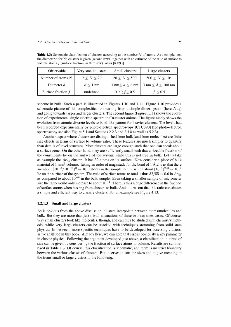
Table 1.3: Schematic classification of clusters according to the number N of atoms. As a complementthe diameter d for Na clusters is given (second row), together with an estimate of the ratio of surface tovolume atoms f (surface fraction, in third row). After [KV93].

Observable Very small clusters Small clusters Large clusters

Number of atoms N 2 ≤ N ≤ 20 20 ≤ N ≤ 500 500 ≤ N ≤ 107

Diameter d d ≤ 1 nm 1 nm≤ d ≤ 3 nm 3 nm ≤ d ≤ 100 nm

Surface fraction f undefined 0.9 >∼f >∼ 0.5 f ≤ 0.5

scheme in bulk. Such a path is illustrated in Figures 1.10 and 1.11. Figure 1.10 provides aschematic picture of this complexification starting from a simple dimer system (here Na2)and going towards larger and larger clusters. The second figure (Figure 1.11) shows the evolu-tion of experimental single electron spectra in Cu cluster anions. The figure nicely shows theevolution from atomic discrete levels to band-like pattern for heavier clusters. The levels hadbeen recorded experimentally by photo-electron spectroscopy [CTCS90] (for photo-electronspectroscopy see also Figure 5.1 and Sections 2.2.3 and 2.3.8 as well as 5.2.3).

Another aspect where clusters are distinguished from bulk (and from molecules) are finitesize effects in terms of surface to volume ratio. These features are much simpler to quantifythan details of level structure. Most clusters are large enough such that one can speak abouta surface zone. On the other hand, they are sufficiently small such that a sizeable fraction ofthe constituents lie on the surface of the system, while this is not true in bulk. Let us takeas example the Ar55 cluster. It has 32 atoms on its surface. Now consider a piece of bulkmaterial of 1 mm3 volume. Taking an order of magnitude for the bond of 1 Atells us that thereare about (10−3/10−10)3 ∼ 1018 atoms in the sample, out of which about (1018)2/3 ∼ 1012

lie on the surface of the system. The ratio of surface atoms to total is thus 32/55 ∼ 0.6 in Ar55

as compared to about 10−6 in the bulk sample. Even taking a smaller sample of micrometersize the ratio would only increase to about 10−4. There is thus a huge difference in the fractionof surface atoms when passing from clusters to bulk. And it turns out that this ratio constitutesa simple and efficient way to classify clusters. For an example see Figure 4.13.

1.2.1.3 Small and large clusters

As is obvious from the above discussion, clusters interpolate between atoms/molecules andbulk. But they are more than just trivial emanations of these two extremes cases. Of course,very small clusters look like molecules, though, and can thus be studied with chemistry meth-ods, while very large clusters can be attacked with techniques stemming from solid statephysics. In between, more specific techniques have to be developed for accessing clusters,as we shall see in this book. Already here, we can note that size is obviously a key parameterin cluster physics. Following the argument developed just above, a classification in terms ofsize can be given by considering the fraction of surface atoms to volume. Results are summa-rized in Table 1.3. Of course, this classification is schematic, and there is no strict boundarybetween the various classes of clusters. But it serves to sort the sizes and to give meaning tothe terms small or large clusters in the following.

26 1 About clusters

The question of size effects will be recurrent throughout this book, first, because clustersinterpolate between atom and bulk with largely variable size, and second, because it turnsout that most cluster properties do indeed strongly depend on size. But as already stressedabove, convergence towards the bulk value with increasing cluster size essentially dependson the nature of the observable and on the resolution with which one looks at it. The bestexplanation is to consider a few examples. The experimental resolution of photo-electronspectra puts the transition from well separated discrete electron levels to quasi-continuousbands at about N ≈ 100. Electronic shell effects, as e.g. magic HOMO-LUMO gaps, shrink∝ N−1/3. And yet, their importance has triggered large efforts to resolve these up to the rangeof N ≈ 3000, see Section 4.2.1.1. Atomic shell effects have been resolved up to N ≈ 10000,see Section 4.2.1.2. The peak frequency of optical response converges also towards its bulkvalue with a term linear in N−1/3. This means that colors keep drifting with size up to verylarge clusters in the range > 10000, see Figure 1.17 in Section 1.3.3.2. The cluster radiusreaches the wavelength of visible light typically around N ≈ 109, while the treatment ofphoto-excitation in the limit of long wavelengths is to be questioned much earlier. Many otherexamples will be found in this book.

1.2.2 Varying cluster material

There are, of course, various types of clusters in terms of bonding, depending on the nature ofthe atoms entering the cluster. As we have seen above, simple molecules as well as bulk canbe grouped into the same four classes of bonds: metallic, covalent, ionic, and van-der-Waalsbonding. It is natural then to classify bonding in clusters according to these four classes. Andthis turns out to constitute an important and relevant means for the classification of clusters.It also reflects deeper physical processes, even if these processes may sometimes differ fromthe ones observed either in molecules or in the bulk. The case of metalicity and its definitionin terms of electron delocalization is a typical example of such a much debated criterion.

The first figure of this book, namely Figure 1.1, shows the famous C60 fullerene whichprovides a beautiful example of covalent bonding in clusters. In that case the cluster exhibitsa well defined structure with electrons localized along the various links between the atoms.As expected, and as observed, other clusters made out of atoms of the carbon group exhibitcovalent bonding as well, consider e.g., the case of the silicon clusters [Sug98].

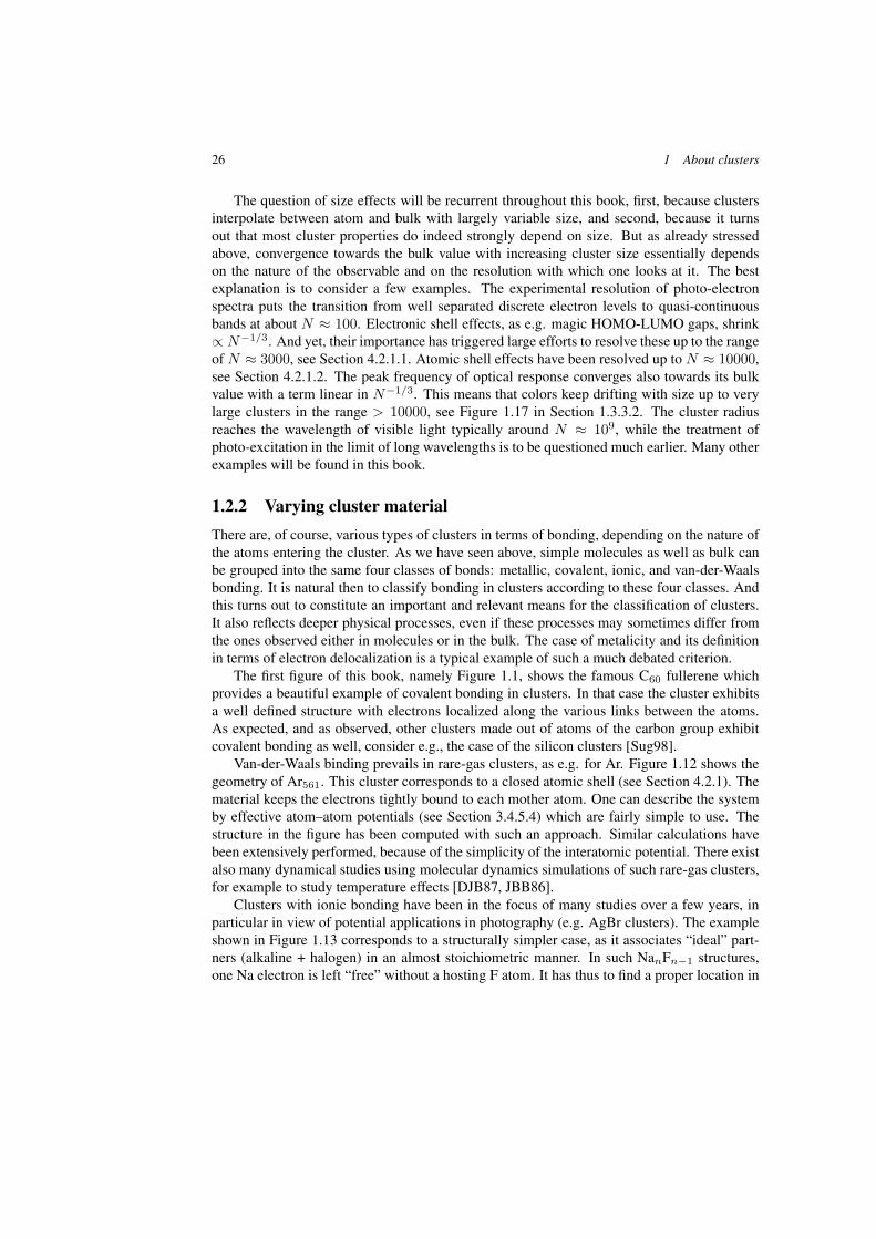
Van-der-Waals binding prevails in rare-gas clusters, as e.g. for Ar. Figure 1.12 shows thegeometry of Ar561. This cluster corresponds to a closed atomic shell (see Section 4.2.1). Thematerial keeps the electrons tightly bound to each mother atom. One can describe the systemby effective atom–atom potentials (see Section 3.4.5.4) which are fairly simple to use. Thestructure in the figure has been computed with such an approach. Similar calculations havebeen extensively performed, because of the simplicity of the interatomic potential. There existalso many dynamical studies using molecular dynamics simulations of such rare-gas clusters,for example to study temperature effects [DJB87, JBB86].

Clusters with ionic bonding have been in the focus of many studies over a few years, inparticular in view of potential applications in photography (e.g. AgBr clusters). The exampleshown in Figure 1.13 corresponds to a structurally simpler case, as it associates “ideal” part-ners (alkaline + halogen) in an almost stoichiometric manner. In such NanFn−1 structures,one Na electron is left “free” without a hosting F atom. It has thus to find a proper location in

1.2 Clusters between atom and bulk 27

Figure 1.12: Geometrical configuration of theAr561 cluster computed by simulated annealing (Sec-tion 3.4.3.2 and Appendix H.3) with effective atom–atom potentials. After [Hab94].

the cluster. Systematic studies in NanFn−1 clusters have shown that there basically exist fourtypes of ionic structures corresponding to four different localizations of the excess electronprovided by the excess Na atom. As illustrated in Figure 1.13, the regular NaF ionic structureclearly shines through, whatever the detail of the arrangement and the location of the excesselectron. This regular ionic structure already appears in very small clusters such as Na5F4. Inthat particular case the excess electron remains localized around the “isolated” sodium atom,but there are other cases in which the electron may spread over a larger fraction of the structuresuch as for example in Na14F13.

The last class of clusters is made out of atoms which exhibit metallic bonding. The sim-plest example is here the case of alkaline atoms for which the metallic behavior is well as-sessed and simple to work out. Figure 1.14 shows the Na4 cluster. It has a planar geometrywhich makes plotting and viewing simpler. Both electron density and ionic positions are ex-plicitly represented. As expected in a metallic system, the electronic density extends more orless smoothly over the whole system. The small Na4 cluster exhibits a clearly oblate shape.Correlatively, the electron cloud is strongly oblate, with a shape very similar to the ionic shape.The shape is determined here by electronic shell structure as discussed in Section 4.2.2.2.Larger metal clusters tend to favor spherical shapes due to the surface tension of the electroncloud. Crystalline shapes may emerge at very low temperature and/or for non-simple metals[Mar93]. In any case, the electrons have a large mobility and behave almost like an electrongas in a (spherical) container. Large metal clusters thus provide an ideal basis for the real-ization of the old Mie idea on the optical response of metallic spheres. This will be outlinedbelow in Section 1.3.3. But before focusing on optical response of metal clusters let us brieflysummarize our conclusions on the different types of binding.

A summary of the four classes of bonding and some of their consequences for clusterproperties is presented in Table 1.4. It continues the energetic considerations of Section 1.1.2.4on the dimer molecules. We recall the word of caution from Section 1.1 that such sortingschemes rely on idealizations and that reality falls often in between the categories. With that inmind, we can benefit from the table. We see that the least bound clusters are van-der-Waals (ormolecular) clusters. They can be considered as a collection of weakly interacting atoms. The

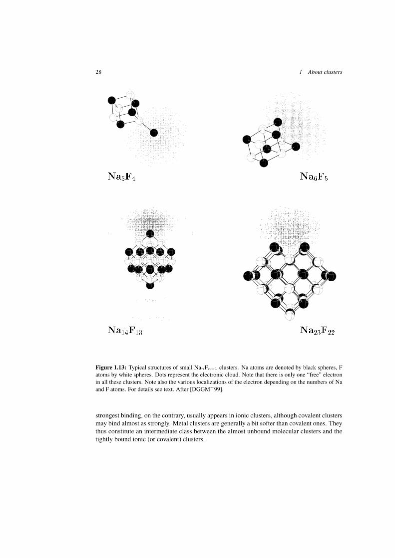
28 1 About clusters

����� �����

������� �������

Figure 1.13: Typical structures of small NanFn−1 clusters. Na atoms are denoted by black spheres, Fatoms by white spheres. Dots represent the electronic cloud. Note that there is only one “free” electronin all these clusters. Note also the various localizations of the electron depending on the numbers of Naand F atoms. For details see text. After [DGGM+99].

strongest binding, on the contrary, usually appears in ionic clusters, although covalent clustersmay bind almost as strongly. Metal clusters are generally a bit softer than covalent ones. Theythus constitute an intermediate class between the almost unbound molecular clusters and thetightly bound ionic (or covalent) clusters.

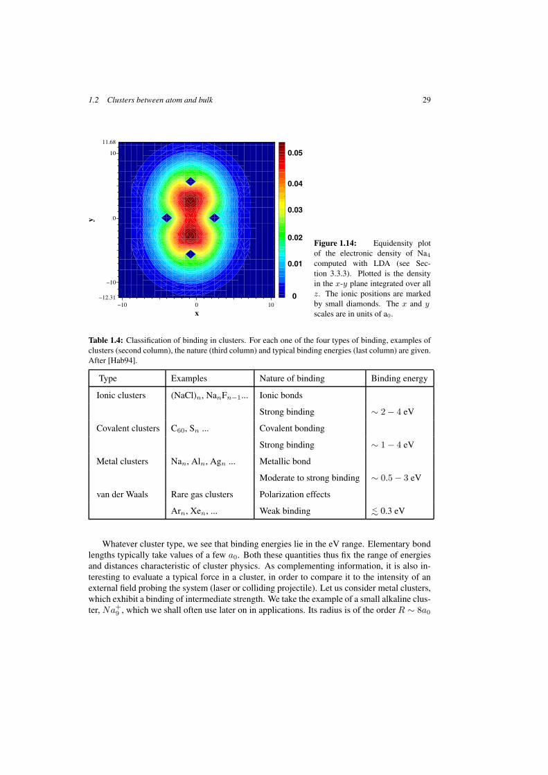
1.2 Clusters between atom and bulk 29

−10 0 10−12.31

−10

0

10

11.68

Na4_22

x

y

0

0.00318

0.00637

0.00955

0.0127

0.0159

0.0191

0.0223

0.0255

0.0287

0.0318

0.035

0.0382

0.0414

0.0446

0.0478

0.05090.05

0.04

0.03

0.02

0.01

0

Figure 1.14: Equidensity plotof the electronic density of Na4

computed with LDA (see Sec-tion 3.3.3). Plotted is the densityin the x-y plane integrated over allz. The ionic positions are markedby small diamonds. The x and yscales are in units of a0.

Table 1.4: Classification of binding in clusters. For each one of the four types of binding, examples ofclusters (second column), the nature (third column) and typical binding energies (last column) are given.After [Hab94].

Type Examples Nature of binding Binding energy

Ionic clusters (NaCl)n, NanFn−1... Ionic bonds

Strong binding ∼ 2 − 4 eV

Covalent clusters C60, Sn ... Covalent bonding

Strong binding ∼ 1 − 4 eV

Metal clusters Nan, Aln, Agn ... Metallic bond

Moderate to strong binding ∼ 0.5 − 3 eV

van der Waals Rare gas clusters Polarization effects

Arn, Xen, ... Weak binding <∼ 0.3 eV

Whatever cluster type, we see that binding energies lie in the eV range. Elementary bondlengths typically take values of a few a0. Both these quantities thus fix the range of energiesand distances characteristic of cluster physics. As complementing information, it is also in-teresting to evaluate a typical force in a cluster, in order to compare it to the intensity of anexternal field probing the system (laser or colliding projectile). Let us consider metal clusters,which exhibit a binding of intermediate strength. We take the example of a small alkaline clus-ter, Na+

9 , which we shall often use later on in applications. Its radius is of the order R ∼ 8a0

30 1 About clusters

and we can estimate the typical electric field at surface as E0 ∼ e2/R2 ∼ 3.4 eV/a0. Suchan electric field corresponds to a laser intensity I ≈ 1013−14W/cm−2 (Section 4.1.1.1). Thatmeans that non-destructive analysis of clusters by light has to be performed with laser intensi-ties much below this value. In turn, with laser intensities of that order or larger, one will mostprobably destroy the cluster. For a more detailed view see Figure 3.3.

1.3 Metal clusters

1.3.1 Some specific properties

Metal clusters play a particularly pronounced role in cluster physics. They have attracted manyinvestigators and the number of publications on that topic stays above average as comparedto other materials. They will also appear quite often as examples throughout this book. Thisimportance of metals is not the sole privilege of cluster physics. Following the introductoryremarks of a famous book in solid state physics [AM76], one may recall that nature seemsto have a “preference” for metals. More than two thirds of the elements are indeed metals.Furthermore, the understanding of metallic behavior turns out to constitute a key issue tounderstand the properties of solids, both conductors and insulators. Finally, as already pointedout before, the characteristic scalability of clusters finds particularly nice applications in thecase of metal clusters. Electrons do form there a quasi free gas with generic properties, whichlead to reasonably well understood behaviors with respect to size.

The features which make metals so different is the long mean free path of the valenceelectrons and the low melting point, ideally realized in alkalines and here at its best for Na.The nearly free propagation of the electrons throughout the cluster constitutes a generic testlaboratory for the physics of an electron cloud, to be more precise, for a finite many-fermionsystem in the degenerate regime. The ionic background serves to deliver the finite bounds.Details of ionic structure can be easily wiped out, if necessary, by handling the cluster abovethe melting point. In other words, metal clusters are a near to perfect realization of a quantumsystem with self-adjusting bounds and shapes. One prominent consequence of the mobileelectron cloud is a strong coupling to light with pronounced resonant behavior, the well knownMie surface plasmon resonance. We shall come back to this point at many places in this book.A first discussion in very simple terms is given in Section 1.3.3. The quantum mechanics ofa confined electron cloud is dominated by shell effects. Metal clusters with their arbitrarilyscalable size have provided here for the first time a laboratory to detect quantum mechanicalshell effects up to system sizes of several thousands of fermions and with it shell beating andsuper-shells, see Section 4.2.1.1. The self-adjusting shape, as opposed to the fixed shapes ofa quantum dot in a substrate, also delivers brilliant examples for the Jahn-Teller effect, as willbe discussed in Section 4.2.2.2.

For pedagogical reasons we will thus use at many places throughout this book resultsobtained with metal clusters. This is motivated by two reasons. First, it does reflect the relativeimportance of metal clusters in experimental and theoretical investigations. Second, referringto the same test case at different places makes the links between the various approaches andapplications more transparent. This makes the whole presentation more coherent and selfcontained. This can be seen, e.g., with respect to time scales. They will obviously play a

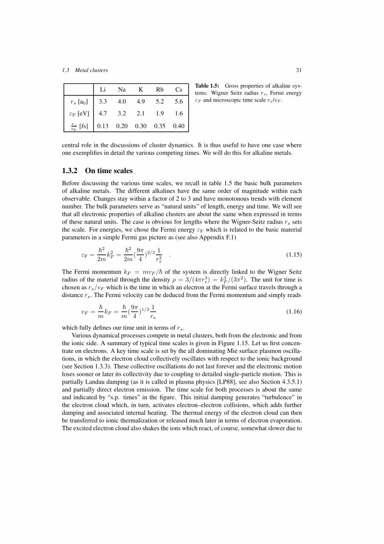
1.3 Metal clusters 31

Li Na K Rb Cs

rs [a0] 3.3 4.0 4.9 5.2 5.6

εF [eV] 4.7 3.2 2.1 1.9 1.6

rs

vF[fs] 0.13 0.20 0.30 0.35 0.40

Table 1.5: Gross properties of alkaline sys-tems: Wigner Seitz radius rs, Fermi energyεF and microscopic time scale rs/vF .

central role in the discussions of cluster dynamics. It is thus useful to have one case whereone exemplifies in detail the various competing times. We will do this for alkaline metals.

1.3.2 On time scales

Before discussing the various time scales, we recall in table 1.5 the basic bulk parametersof alkaline metals. The different alkalines have the same order of magnitude within eachobservable. Changes stay within a factor of 2 to 3 and have monotonous trends with elementnumber. The bulk parameters serve as “natural units” of length, energy and time. We will seethat all electronic properties of alkaline clusters are about the same when expressed in termsof these natural units. The case is obvious for lengths where the Wigner-Seitz radius rs setsthe scale. For energies, we chose the Fermi energy εF which is related to the basic materialparameters in a simple Fermi gas picture as (see also Appendix F.1)

εF =�

2

2mk2

F =�

2

2m(9π

4)2/3 1

r2s

. (1.15)

The Fermi momentum kF = mvF /� of the system is directly linked to the Wigner Seitzradius of the material through the density ρ = 3/(4πr3

s) = k3F /(3π2). The unit for time is

chosen as rs/vF which is the time in which an electron at the Fermi surface travels through adistance rs. The Fermi velocity can be deduced from the Fermi momentum and simply reads

vF =�

mkF =

�

m(9π

4)1/3 1

rs(1.16)

which fully defines our time unit in terms of rs.Various dynamical processes compete in metal clusters, both from the electronic and from

the ionic side. A summary of typical time scales is given in Figure 1.15. Let us first concen-trate on electrons. A key time scale is set by the all dominating Mie surface plasmon oscilla-tions, in which the electron cloud collectively oscillates with respect to the ionic background(see Section 1.3.3). These collective oscillations do not last forever and the electronic motionloses sooner or later its collectivity due to coupling to detailed single-particle motion. This ispartially Landau damping (as it is called in plasma physics [LP88], see also Section 4.3.5.1)and partially direct electron emission. The time scale for both processes is about the sameand indicated by “s.p. times” in the figure. This initial damping generates “turbulence” inthe electron cloud which, in turn, activates electron–electron collisions, which adds furtherdamping and associated internal heating. The thermal energy of the electron cloud can thenbe transferred to ionic thermalization or released much later in terms of electron evaporation.The excited electron cloud also shakes the ions which react, of course, somewhat slower due to

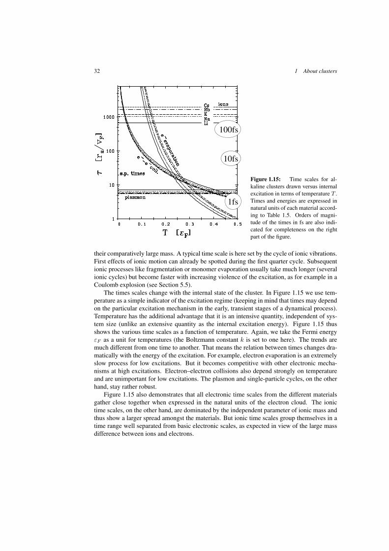
32 1 About clusters

1fs

10fs

100fs

Figure 1.15: Time scales for al-kaline clusters drawn versus internalexcitation in terms of temperature T .Times and energies are expressed innatural units of each material accord-ing to Table 1.5. Orders of magni-tude of the times in fs are also indi-cated for completeness on the rightpart of the figure.

their comparatively large mass. A typical time scale is here set by the cycle of ionic vibrations.First effects of ionic motion can already be spotted during the first quarter cycle. Subsequentionic processes like fragmentation or monomer evaporation usually take much longer (severalionic cycles) but become faster with increasing violence of the excitation, as for example in aCoulomb explosion (see Section 5.5).

The times scales change with the internal state of the cluster. In Figure 1.15 we use tem-perature as a simple indicator of the excitation regime (keeping in mind that times may dependon the particular excitation mechanism in the early, transient stages of a dynamical process).Temperature has the additional advantage that it is an intensive quantity, independent of sys-tem size (unlike an extensive quantity as the internal excitation energy). Figure 1.15 thusshows the various time scales as a function of temperature. Again, we take the Fermi energyεF as a unit for temperatures (the Boltzmann constant k is set to one here). The trends aremuch different from one time to another. That means the relation between times changes dra-matically with the energy of the excitation. For example, electron evaporation is an extremelyslow process for low excitations. But it becomes competitive with other electronic mecha-nisms at high excitations. Electron–electron collisions also depend strongly on temperatureand are unimportant for low excitations. The plasmon and single-particle cycles, on the otherhand, stay rather robust.

Figure 1.15 also demonstrates that all electronic time scales from the different materialsgather close together when expressed in the natural units of the electron cloud. The ionictime scales, on the other hand, are dominated by the independent parameter of ionic mass andthus show a larger spread amongst the materials. But ionic time scales group themselves in atime range well separated from basic electronic scales, as expected in view of the large massdifference between ions and electrons.

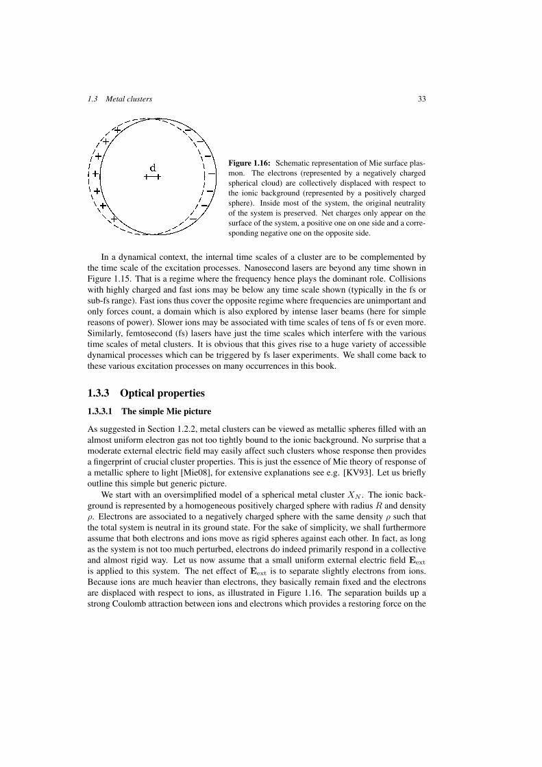
1.3 Metal clusters 33

Figure 1.16: Schematic representation of Mie surface plas-mon. The electrons (represented by a negatively chargedspherical cloud) are collectively displaced with respect tothe ionic background (represented by a positively chargedsphere). Inside most of the system, the original neutralityof the system is preserved. Net charges only appear on thesurface of the system, a positive one on one side and a corre-sponding negative one on the opposite side.

In a dynamical context, the internal time scales of a cluster are to be complemented bythe time scale of the excitation processes. Nanosecond lasers are beyond any time shown inFigure 1.15. That is a regime where the frequency hence plays the dominant role. Collisionswith highly charged and fast ions may be below any time scale shown (typically in the fs orsub-fs range). Fast ions thus cover the opposite regime where frequencies are unimportant andonly forces count, a domain which is also explored by intense laser beams (here for simplereasons of power). Slower ions may be associated with time scales of tens of fs or even more.Similarly, femtosecond (fs) lasers have just the time scales which interfere with the varioustime scales of metal clusters. It is obvious that this gives rise to a huge variety of accessibledynamical processes which can be triggered by fs laser experiments. We shall come back tothese various excitation processes on many occurrences in this book.

1.3.3 Optical properties

1.3.3.1 The simple Mie picture

As suggested in Section 1.2.2, metal clusters can be viewed as metallic spheres filled with analmost uniform electron gas not too tightly bound to the ionic background. No surprise that amoderate external electric field may easily affect such clusters whose response then providesa fingerprint of crucial cluster properties. This is just the essence of Mie theory of response ofa metallic sphere to light [Mie08], for extensive explanations see e.g. [KV93]. Let us brieflyoutline this simple but generic picture.

We start with an oversimplified model of a spherical metal cluster XN . The ionic back-ground is represented by a homogeneous positively charged sphere with radius R and densityρ. Electrons are associated to a negatively charged sphere with the same density ρ such thatthe total system is neutral in its ground state. For the sake of simplicity, we shall furthermoreassume that both electrons and ions move as rigid spheres against each other. In fact, as longas the system is not too much perturbed, electrons do indeed primarily respond in a collectiveand almost rigid way. Let us now assume that a small uniform external electric field Eext

is applied to this system. The net effect of Eext is to separate slightly electrons from ions.Because ions are much heavier than electrons, they basically remain fixed and the electronsare displaced with respect to ions, as illustrated in Figure 1.16. The separation builds up astrong Coulomb attraction between ions and electrons which provides a restoring force on the

34 1 About clusters

displaced electron cloud counteracting eEext. Denoting by d the actual separation of ionicand electronic center of masses the net force acting on the electron cloud (along the directionof Eext) reads for small d

F = −N4πρe2

3d = NEext . (1.17)

Once the external perturbation is switched off, there only remains the attractive force betweenelectrons and ions. This force is proportional to the actual separation d between ions andelectrons. The mobile part of the system is the electron cloud having total mass Nmel. It willthus undergo harmonic oscillations around ions, with a frequency

ω2Mie =

4πρe2

3mel=

e2

melr3s

(1.18)

where mel is the electron mass. This oscillation frequency is known as the Mie frequency.When a cluster is irradiated by light the situation is about the same as described above.

Optical wavelengths range in the micrometer domain, which is much larger than most clustersizes. The electrical field is thus locally uniform at the cluster site and provokes the abovedescribed collective oscillation of the electron cloud against the ionic background. The typ-ical values of ωMie for simple alkaline metals lie in the visible part of the electromagneticspectrum, whence the term “optical response” to characterize this phenomenon. For the al-kalines, whose rs were given in table 1.5, the Mie frequencies are: �ωMie(Li) = 4.5 eV,�ωMie(Na) = 3.4 eV, �ωMie(K) = 2.5 eV, �ωMie(Rb) = 2.3 eV, and �ωMie(Cs) = 2.1eV. These estimates fit fairly well with experimental values as we will see later. The rela-tions are more involved for non-simple metals as, e.g., noble metals. There one needs to takethe polarizability of the core electrons into account (see Section 1.3.3.2 and the discussion inSection 4.3.4.1).

1.3.3.2 The dielectric picture

The explicit picture of an oscillating electron cloud led to the expression (1.18) of the Miefrequency simply in terms of bulk density ρ. In more involved materials one needs to accountfor internal polarizability. This can be done at the level of macroscopic models by employingthe bulk dielectric constant of the medium ε. Note that dielectric media require one to makea distinction between an externally applied electrical field Eext and the effective internal fieldEint which emerges when cumulating the additional fields from internal polarization effects.The external field is directly related to the external sources while the internal field describesthe net effect on moving charges, accounting for both external sources and induced charges.Both are related at a macroscopic level through the standard relation

Eint(r, ω) = ε(r, ω)Eext(r, ω) . (1.19)

This relation is given for the dynamical polarizability ε(r, ω) which is more easily formulatedin terms of frequency ω of the applied field. Transformation to the time domain yields apolarizability with memory kernel depending on all past times. The space dependence can be

1.3 Metal clusters 35

omitted in homogeneous materials. But it plays a crucial role at interfaces between differentmaterials.

Clusters are finite systems with a large surface area. Let us thus consider a finite piece,namely a spherical sampling, of the bulk material with given dielectricity ε. The response ofthat dielectric sphere to a homogeneous external electrical field can be worked out with stan-dard techniques of electro-dynamics (see e.g. [Jac62, KV93]). The result for this sphericallysymmetric system is

Eint =3

2 + εEext . (1.20)

The Mie resonance frequency is found at the point where the internal field becomes self-supporting, i.e. where we can have a finite Eint for zero excitation Eext. This defines theresonance frequency ωMie through

2 + ε(ωMie) = 0 . (1.21)

That definition holds for a much broader class of metals than the simpler relation (1.18). Theprice is that one has to know the whole bulk ε(ω).

In the following, we want to show that the definition (1.21) becomes identical with (1.18)for the case of simple metals. To that end, we have first to develop a simple model for the bulkdielectric constant. Let us thus consider an “infinite” piece of metal irradiated by an externallight source. The external electric field polarizes the medium. The effect can be estimated atan elementary level by considering the motion of a single electron subject to the net electricfield Eint. The electron follows the Newtonian equation of motion

md2rdt2

= −eEint . (1.22)

For a sinusoidal electric field of frequency ω, the solution is also sinusoidal with the samefrequency. The polarization of the medium then simply reads

P = −ρer = − ρe2

mω2Eint (1.23)

from which one deduces the total field Eint = Eext +P = εEext and the frequency dependentdielectric function

ε(ω) = 1 − ω2p

ω2, ωp =

√4πρe2

mel=

√3e2

melr3s

(1.24)

where ωp is the bulk plasma frequency of the medium. The plasma frequency is related toε = 0. It characterizes the point of infinite response in bulk, i.e. an eigenmode of bulkoscillations. The infinite response never occurs in practice. Damping processes take overfar before the amplitude explodes. The damping can be taken into account by introducingone relaxation time τ at the present level of estimate. This generalizes the above dielectricresponse to the Drude model [AM76], giving ε = 1 − ω2

pτ/(ω(ı + ωτ )) which merges intothe form Eq. (1.24) for the limit τ −→ ∞.

36 1 About clusters

Let us now insert the dielectric function Eq. (1.24) into the condition Eq. (1.21) for a Mieplasmon. This yields with a bit of simple algebra ωMie = ωp/

√3 and thus precisely the

frequency (1.18). This bulk-oriented approach thus allows one to recover the simple relationfor the Mie frequency when using a spherical dielectric. The macroscopic treatment can easilybe extended to more general shapes as, e.g., spheroidal clusters and allows one here to sorta lot of global phenomena. This line is followed to a large extend in [KV93]. In this book,however, we will put more weight on the microscopic treatment as outlined in Chapter 3.

As is clear from the above discussion, in a finite system electron oscillations will domi-nantly show up at the surface of the system, while in bulk they manifest themselves throughelectron density oscillations at plasma frequency ωp, independent from the surface. In factboth mechanisms do exist in finite systems like clusters. In other words, an electric field in-duces both electron displacement and electron density fluctuations. It simply turns out that ina finite system the surface effect dominates over the bulk effect and one thus mostly observesthe surface response, theoretically as well as experimentally. This means that photoabsorp-tion spectra of the optical response of metal clusters to light are dominated by the surfaceplasmon, while a, usually much suppressed, contribution from the so called volume plasmon(corresponding to the bulk-like response) may be spotted in the frequency domain around

√3

times the surface plasmon.The existence of a resonance such as the Mie plasmon (or the volume plasmon) has im-

portant consequences on the way the system will actually couple to light. To make the pointspecific let us consider the case of a cluster subject to a laser irradiation, a situation that weshall encounter at many places along this book. In this case, one can easily estimate theamount of absorbed laser power by the system by simply considering the motion of individualelectrons subject to the laser field of frequency ωlas and the damped (with relaxation time τ )plasmon oscillations of frequency ωMie (following, in that respect the simplest Drude model).The instantaneous absorbed power can be expressed as Pabs = −eρvE averaged over all pos-sible electron velocities v. Time averaging over one laser cycle, one obtains the well knownresonant absorption form

< Pabs >= P0u2

(1 − u2)2 + (u/ωMieτ )2(1.25)

where u = ωlas/ωMie. The above form obviously exhibits a resonance at ωlas/ωMie. Thismeans that when irradiating a cluster with a laser field one should expect resonant energyabsorption when the laser frequency comes close to the plasmon frequency. This resonantbehavior will actually be observed and exploited in many situations all along this book (see inparticular the discussion in Section 5.3.1.1).

1.3.3.3 Optical response in metal clusters

The Mie model and the dielectric approach, outlined above, show that metals resonantly cou-ple to light, both in bulk as well as in small particles. In finite systems such as clusters, thesurface plasmon dominates the response and we shall mostly focus on this aspect in the fol-lowing. The resonance frequencies provided by the above models, Eqs. (1.18) or (1.24), areindependent of cluster size. This does not fully agree with experimentally observed responsespectra. Figure 1.17 shows optical absorption spectra of deposited clusters of various sizes.

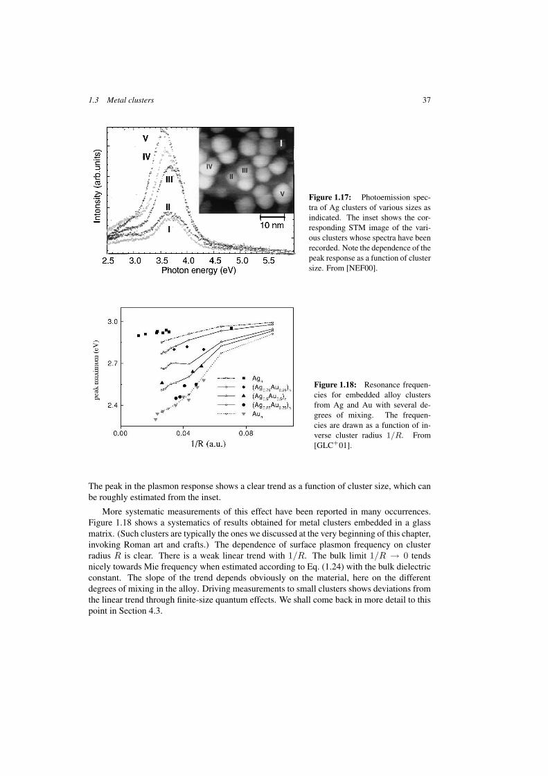
1.3 Metal clusters 37

Figure 1.17: Photoemission spec-tra of Ag clusters of various sizes asindicated. The inset shows the cor-responding STM image of the vari-ous clusters whose spectra have beenrecorded. Note the dependence of thepeak response as a function of clustersize. From [NEF00].

Figure 1.18: Resonance frequen-cies for embedded alloy clustersfrom Ag and Au with several de-grees of mixing. The frequen-cies are drawn as a function of in-verse cluster radius 1/R. From[GLC+01].

The peak in the plasmon response shows a clear trend as a function of cluster size, which canbe roughly estimated from the inset.

More systematic measurements of this effect have been reported in many occurrences.Figure 1.18 shows a systematics of results obtained for metal clusters embedded in a glassmatrix. (Such clusters are typically the ones we discussed at the very beginning of this chapter,invoking Roman art and crafts.) The dependence of surface plasmon frequency on clusterradius R is clear. There is a weak linear trend with 1/R. The bulk limit 1/R → 0 tendsnicely towards Mie frequency when estimated according to Eq. (1.24) with the bulk dielectricconstant. The slope of the trend depends obviously on the material, here on the differentdegrees of mixing in the alloy. Driving measurements to small clusters shows deviations fromthe linear trend through finite-size quantum effects. We shall come back in more detail to thispoint in Section 4.3.

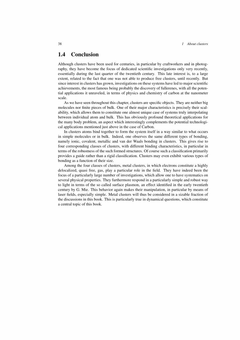
38 1 About clusters

1.4 Conclusion

Although clusters have been used for centuries, in particular by craftworkers and in photog-raphy, they have become the focus of dedicated scientific investigations only very recently,essentially during the last quarter of the twentieth century. This late interest is, to a largeextent, related to the fact that one was not able to produce free clusters, until recently. Butsince interest in clusters has grown, investigations on these systems have led to major scientificachievements, the most famous being probably the discovery of fullerenes, with all the poten-tial applications it unraveled, in terms of physics and chemistry of carbon at the nanometerscale.

As we have seen throughout this chapter, clusters are specific objects. They are neither bigmolecules nor finite pieces of bulk. One of their major characteristics is precisely their scal-ability, which allows them to constitute one almost unique case of systems truly interpolatingbetween individual atom and bulk. This has obviously profound theoretical applications forthe many body problem, an aspect which interestingly complements the potential technologi-cal applications mentioned just above in the case of Carbon.

In clusters atoms bind together to form the system itself in a way similar to what occursin simple molecules or in bulk. Indeed, one observes the same different types of bonding,namely ionic, covalent, metallic and van der Waals bonding in clusters. This gives rise tofour corresponding classes of clusters, with different binding characteristics, in particular interms of the robustness of the such formed structures. Of course such a classification primarilyprovides a guide rather than a rigid classification. Clusters may even exhibit various types ofbonding as a function of their size.

Among the four classes of clusters, metal clusters, in which electrons constitute a highlydelocalized, quasi free, gas, play a particular role in the field. They have indeed been thefocus of a particularly large number of investigations, which allow one to have systematics onseveral physical properties. They furthermore respond in a particularly simple and robust wayto light in terms of the so called surface plasmon, an effect identified in the early twentiethcentury by G. Mie. This behavior again makes their manipulation, in particular by means oflaser fields, especially simple. Metal clusters will thus be considered in a sizable fraction ofthe discussions in this book. This is particularly true in dynamical questions, which constitutea central topic of this book.