_1 _epartme.tofAgri©ulture

_°_e'Sc'e|dentifying PublicNorth Central

Ft°atlStnExperiment Research Priorities:General TechnicalReport NC-109 ! a S

An App|_cat_on _nForestry ResearchGlenn Fox

J

_' ..... .. - ...... -. _ -

...... . ....... -- - . -_a

CONTENTS

Page

Economic Models for Assessing Research Priorities ............. 1Introduction and Overview ................................. 1

Scoring Models and Multiple Goal Linear Programming ...... 2An LP Model for Evaluating Research Projects ............... 5Precedence and Congruence ................................ 6Dynamic Cost-Benefit Models ............................... 7Models of Regional Spillover Effects ......................... 10Optimal Growth Models .................................... 11

Identifying Southern Pine Forestry Research Priorities ......... 14Background ............................................... 14Congruence Calculations ................................... 14A Social Surplus Model of Research Resource Allocation ...... 15

References ................................................... 19

North Central Forest Experiment StationForest ServicemU.S. Department of Agriculture

1992 Folwell AvenueSt. Paul, Minnesota 55108

Manuscript approved for publication June 23, 19861986

A FRAMEWORK FOR IDENTIFYING PUBLIC RESF.. kRCHPRIORITIES: AN

APPLICATION IN FORESTRY RESEARCH 1

Glenn Fox, Assistant Professor,

Department of Agricultural Economics and Business,University of Guelph,

Formerly Research Assistant,Department of Agricultural and Applied Economics,

University of Minnesota

ECONOMIC MODELS FOR posed on the model and the characteristics of solu-tions which emerge, and (2) the information

ASSESSING RESEARCH PRIORITIES required to employ the model for applied researchbudgeting questions.

_troduction and Overview The problem of determining an optimal level ofresearch and development activities within an orga-

In recent decades, major research effort has been nization can be viewed as a component of the overalldevoted to modeling and measuring the relation be- capital budgeting decision. Research competes fortween research and development activity and the resources with the purchase of durable assets andrate and nature of technical change. The notions current inputs and like durable assets and currentthat such change responds, at least in part, to the inputs, contributes to achievement organizationalamount of resources allocated to research, and that goals. While varied techniques have been developed

invention responds to economic incentives, have be- to guide the research resource allocation decision, acome well established. This report reviews efforts to common theme has been an attempt to measure bothmodel optimal research resource allocation, and pre- the degree to which alternative research activitiessents a model for southern pine forestry research, contribute to organizational goals and the opportu-

nity cost of resources devoted to research. The proce-The discussion will focus on two aspects of the dures vary in the formality and detail with which

available models: (1) the general structure of the these measurements are accomplished.optimization procedure, including the objective func-tion to be optimized, the nature of constraints im- Although research funding needs to be seen as

part of the broader capital budgeting process, thenature of research confounds the resource allocation

1While preparing this paper, the author benefitted problem. Perhaps the most outstanding feature offrom discussions with Hans Gregerson, Christopher scientific research as an investment activity is theRisbrudt, Vernon W. Ruttan, and Pamela Jakes. Re- uncertainty inherent in most projects. Ex ante, it issearch support was provided by Minnesota Agricul- never clear how much investment will be required torural Experiment Station Project 14-064, Technical achieve a particular result, and even if success isand Institutional Sources of Change in Agriculture, achieved there is no guarantee that the net contribu-by a Resources for the Future Dissertation Fellowship tion to organizational goals will warrant the invest-Grant in Food and Agricultural Resource Use Policy, ment. Furthermore, because most research organi-and by the U.S. Department of Agriculture, Forest zations have multiple goals, estimatingService, North Central Forest Experiment Station contributions of a research project to specific goals(Cooperative Agreement 23-84-13). and subsequently weighing the goals is difficult.

Scoring Models and Multiple Goal Table 3 reports Russell's criteria. The second panelestablishes scores for each proposed project for eachLinear Programming criterion.

One of the earliest approaches to research budget The weights are then used to construct an ordinalallocation has been called the Scoring model. Panels ranking of projects. Scores are computed either addi-of researchers and administrators identify organiza- tively,tional goals for research, attach weights to goals andto estimate relative contributions to goals of specific J

researchprojects.Thisinformationcan be incorpo- Si- _ Wj Cij

ratedintoa linearprogramming framework by • j=laddingresourcerequirementsofprojectsand meas-

uresoforganizationalresources, ormultiplicatively

A scoringmodelapproachwas usedina nationalassessmentofU.S.agriculturalresearchpriorities J

in 1965 and 1966 (USDA 1966). A similar exercise Si----1--I Wj Cij

was conducted at the state level in North Carolina, j =1beginning in 1972 (Shumway and McCracken 1975).

Russell (1973, 1975) extended a scoring model to a where Si is the score of project i, j is the index forlinear programming approach in the U.K., applying criteria, Wj denotes the weight attached to the jtha framework outlined by Kaldor (1966), Hildreth criterion and Cij is the score of the ith project on the(1966), and Paulson and Kaldor (1968). jth criterion.

This approach usually involves two panels. Thefirst typically consists of senior administrators Russell's approach maximized the linear functionwhose task is to identify a set of organizational goalsfor research and to establish weights for each goal. J

Tables 1 and 2 report the criteria and weights em- _ Wj Cjployed in the USDA and North Carolina studies, j=l

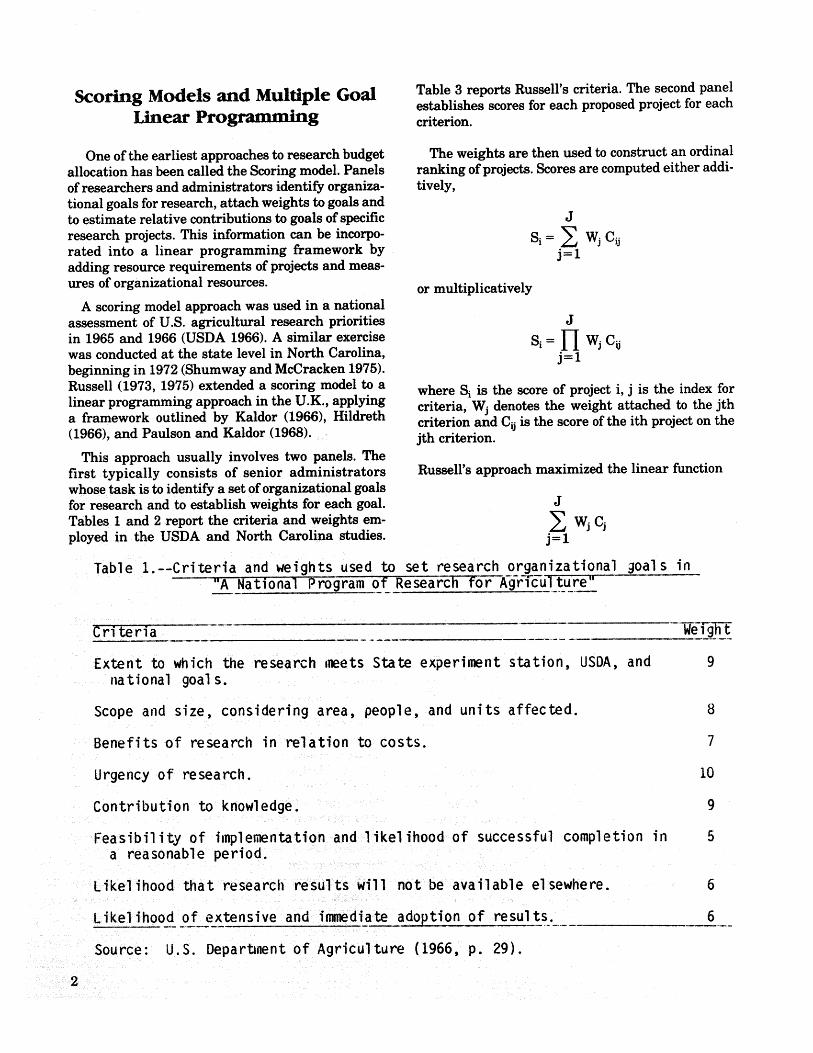
Table 1.--Criteria and weights used to set research organizational _oals in"A National Program of Research for Agrlc-_-uTtu_reu''

Criteria W-e-_-g-h-t

Extent to which the research ineetsState experiment station, USDA, and 9national goals.

Scope and size, considering area, people, and units affected. 8

Benefits of research in relation to costs. 7

Urgency of research. 10

Contribution to knowledge. 9

Feasibility of implementation and likelihood of successful completion in 5a reasonable period.

Likelihood that research results will not be available elsewhere. 6

Likelihood of extensive and immediate adoption of results. 6__

Source: U.S. Deparbnent of Agriculture (1966, p. 29).

2

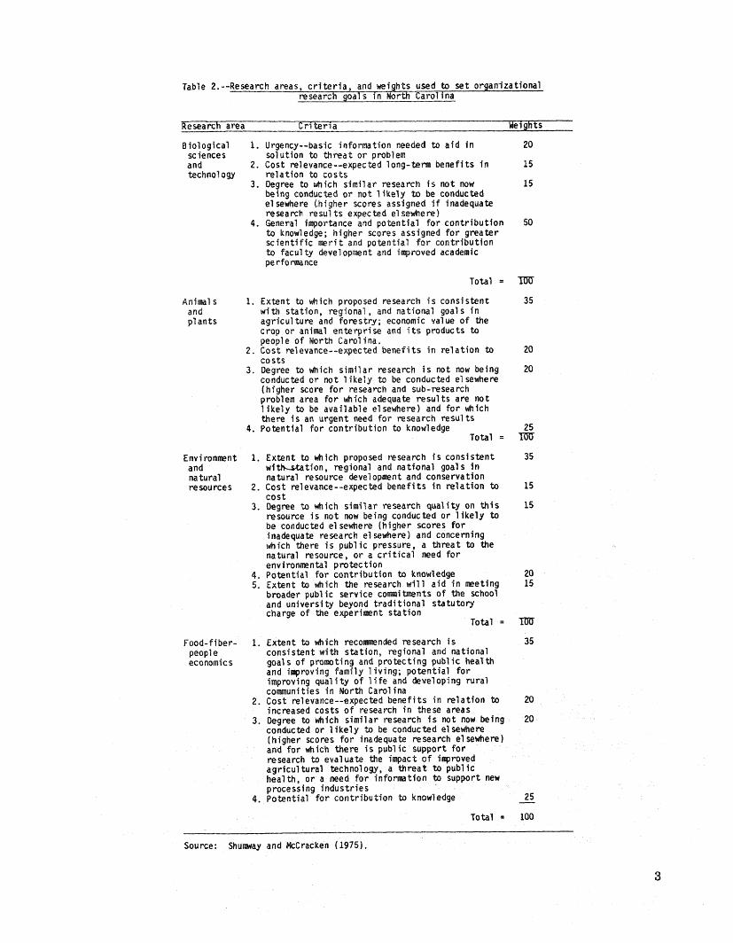
Table 2.--Research areas, criteriaj and wei-hts _sed t0 .setorganizational_-s-earch-_oals in North Carolina

Research area C_a Weights

Biological I. Urgency--basic information needed to aid in 20sciences solution to threat or problemand 2. Cost re]evance--expected long-term benefits in 15technology relation to costs

3. Degree to which similar research is not now 15being conducted or not likely to be conductedelsewhere (,higherscores assigned if inadequateresearch results expected elsewhere)

4. General importance and potential for contribution 50to knowledge; higher scores assigned for greaterscientific merit and potential for contributionto faculty development and improved academicperformance

Total =

Animals I. Extent to which proposed research is consistent 35and with station, regional, and national goals inplants agriculture and forestry; economic value of the

crop or animal enterprise and its products topeople of North Carolina.

2. Cost relevance--expected benefits in relation to ZOcosts

3. Degree to which similar research is not now being 20conducted or not Iikely to be conducted elsewhere(higher score for research and sub-researchproblem area for which adequate results are notlikely to be available elsewhere) and for whichthere is an urgent need for research results

4. Potential for contribution to knowledge 25Total =

Environment I. Extent to which proposed research is consistent 35and with--s_ation,regional and national goals innatural natural resource development and conservationresources 2. Cost relevance--expected benefits in relation to 15

cost

3. Degree to which similar research quality on this 15resource is not now being conducted or likely tobe conducted elsewhere (higher scores forinadequate research elsewhere) and concerning_nich there is public pressure, a threat to thenatural resource, or a critical need forenvironn_ntal protection

4. Potential for contribution to knowledge 205. Extent to which the research will aid in meeting 15

broader public service commitments of the schooland university beyond traditional statutorycharge of the experiment station

Total =

Food-fiber- 1. Extent to which reconrnendedresearch is 35

people consistent with station, regional and nationaleconomics goals of promoting and protecting public health

and improving family living; potential forimproving quality of life and developing ruralcommunities in North Carolina

2. Cost relevance--expected benefits in relation to 20increased costs of research in these areas

3. Degree to which similar research is not now being 20conducted or likely to be conducted elsewhere(higher scores for inadequate research elsewhere)and for which there is public support forresearch to evaluate the impact of improved

agricultural technology, a threat to publichealth, or a need for information to support newprocessing industries

4, Potential for contribution to knowledge 25

Total : I00

Source: Shumway and McCracken (1975).

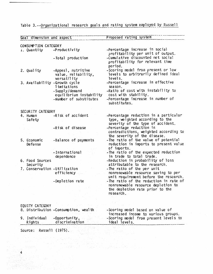
Table 3.--Organizationalresearchgoals and rating systememployedby Russell

G_6_l--__ion anclaspect Proposedr_atingsystem

CONSUNPTIONCATEGORYi. Quantity -Productivity -Percentageincreasein social

profitabilityper unit of output.-Total production -Cumulativediscountednet social

profitabilityfor relevant timeperiod.

2. Quality -Appeal,nutritive -Scoringnmdel frolapresentor lowvalue, reliability, levels to arbitrarilydefined idealversatility levels.

3. Availability-Growthcycle -Percentageincreasein effectivelimitations season.-Supply/de,hand -Ratioof cost with instabilitytoequilibriuminstability cost with stability.-Numberof substitutes -Percentageincreasein number of

substitutes.

SECURITY CATEGORY4. Human -Risk of accident -Percentagereductionin a particular

Safety type,weightedaccordingto theseverityof the type of accident.

-Risk of disease -Percentagereductionincontradictions,weightedaccordingtothe severityof the disease.

5. Economic -Balanceof payments -The ratio of the value of potentialDefense reductionin importsto present value

of imports.-International -The ratio of the expected reductiondependence in trade to total trade.

6. Food Sources -Reductionin probabilityof lossSecurity attributableto the research.

7. Conservation-Utilization -The ratio of the per unitefficiency nonrenewableresourcesaving to per

unit requirementbefore the research.-Depletionrate -The ratio of the reductionin rate of

nonrenewableresourcedepletiontothe depletionrate prior to theresearch.

EQUITY CATEGORY8. Distribution-Consumption,wealth -Scoringmodel based on value of

increasedincometo various groups.9. Individual -Opportunity, -Scoringmodel from presentlevels to

Rights discrimination ideallevels.

Source: Russell (1975).

requirements of projects including any relevant fea-where Cj represents the contribution of all i = 1 to I sibility constraints. The output of the analysis is anprojects to criterion j. Cj is computed as ordinal ranking of projects which can be used to ex-

I haust the research budget. Because the method hasbeen popular in agricultural research as well as in

Cj ----- _ (Cij/ri) ri military and industrial research considerable efforti = 1 has been made to evaluate the technique. Moore and

Baker (1969) in assessing scoring models in militarywhere r i is the level of funding of the ith project and and industrial research, found the advantages of thisr i is an upper limit to the size of the project. The approach to include: (1) broad participation of re-maximization problem is constrained by the total search personnel at several administrative levels,research budget R, (2) limited requirements for technical skills of for-

mal cost-benefit analysis, and (3) explicit identifica-I tion of and relationship to organizational goals.-ri <-R

i= 1 Some of these advantages, however, can also beseen as liabilities. Broad participation can be expen-

and the feasibility constraints sive, particularly in its use of senior administrators'time. The absence of formal benefit-cost calculations

0 _ ri <---ri, i= 1 . . . I. gives an impression of subjectivity and arbitrarinessin the selection of criteria and weights. Also, there is

Work by Fishel (1970, 1971) and Grieg (1979) are no mechanism to weed out redundancy and overlapextensions and adaptations of scoring models. Fishel among criteria. While the relationship to organiza-developed a stochastic cost-benefit model. Rather tional goals is emphasized in this approach, it reallythan seeking expert opinion in the form of scores, gives no guidance in the solution of R, the overallFishel sought estimates of the parameters of a cost- research budget. While in principle an ordinal rank-benefit model. His approach synthesizes subjective ing could be constructed to include all investmentprobability distributions of key variables from panel opportunities available to an institution, this hasand survey data. Researchers and administrators not been done in practice.

were asked to estimate annual costs and benefits In addition, several technical problems remain un-and expected times to completion of several projects, solved. Should Si be computed as an additive or mul-These responses were used to generate point and tiplicative formula? Should project alternatives beinterval estimates of the variables used in the cost- identified on the basis of problem areas, commoditybenefit analysis, groupings or scientific disciplines? Should the varia-

The Fishel approach to measuring benefits com- tion of Si scores among panelists play a role in theputes the sum of the gains in human capital among ordinal ranking? Finally, Moore and Baker reportthe researchers engaged in the project, the present that scoring models are not always able to give sim-salvage value of equipment purchased and the ex- ilar ordinal rankings to cost-benefit procedures.pected net benefits from the knowledge derived.

Grieg developed a stochastic simulation model to All LP Model for Evaluating

study two poultry research projects. Discussions Research Pro_ec_with researchers were used to establish parametersfor a single firm and an aggregate simulation. Theframework developed was quite complex and costly Klein and Kehrberg (1981) have developed ato implement. It was also difficult to independently model to help researchers choose among crossbredverify the information obtained from the research lines at early stages of a livestock breeding program.expert. Extending scoring models to create stochas- In principle, the approach could be applied to planttic cost benefit analysis is fraught with the same breeding, but cost savings would be lower because oflimitations as scoring models in general. It is expen- lower maintenance costs for plants.

sive to accumulate the required data, and validation Linear programming is used to trace a unit iso-is difficult, quant of a crossbred line under alternative factor

Scoring and multiple-goal LP models require a list price regimes. The objective function minimizes unitof potential projects, a set of criteria with associated costs. Results of performance trials of first-weights, and in the programming version resource generation offspring are used to compute an input

requirements matrix, A. Several modes of produc- ri

tion were considered, with each column of A repre-senting the vector of input requirements necessary CRi =to achieve a unit of the production activity. The set PiYi

of production activities, each representing a unique ncombination of housing, feed, and breeding methods, PkYkis represented by the vector L. Total output is repre- X_

k=lsented by yo, and D is a vector of estimates of' outputlevels per unit of each activity in L. Therefore

where ri is the research expenditure on commodity i,DL = yo. Total input use is AL, which must equalR is the total research budget, PiYi is the gross rev-IX, where I is the identity matrix. In summary, the

LP model seeks to enue f_om market sales of commodity i and

Minimize (C + 0)X n

Subject to DL - Y° __j PkYkAL - IX - 0 k= 1

0 is a vector of parameters used to describe alterna- is the gross revenue earned from all commoditiestive factor price regimes, being considered in the research budget. There is an

Ten crossbreeds were compared using the model, ambiguity in this definition in that it is not clear ifSome were found to be of lower unit cost for all factor gross revenue or value added should be employed in

price combinations. Some lines never achieved low- computing CR i.est unit cost for any input price set. The authors Advocates of congruence ratios tend to downplayargued that this information, tempered with the the prescriptive power of the approach. Their use isjudgments of the research team, could be used to seen as a way of relating the size of research expen-identify the most promising crossbred lines for fur- diture to the size of an industry. An important sug-ther investigation. Embryo storage could preserve gestion in these studies is that outliers in the vectorthe genetic material of the least promising cross- of congruence ratios are to be viewed with suspicionbreeds, as being potentially sub optimal. In other words,

congruence ratios should be equal to one unlessthere are "good reasons" for them not to be.

Precedence and Congruence Both the precedence and congruence models havelimited data requirements for implementation. In-

Precedence and congruence models are arguably deed, the precedence approach requires only a copythe least costly means of establishing funding guide- of last year's budget and the size of this year's fund-lines for public research. The precedence approach ing increase or decrease. The congruence model ad-reinforces the status quo. According to this model, ditionally requires information on gross revenues ofthe share of research funds allocated to a particular commodity groups.

commodity remains constant through time. Each Many of the disadvantages of these approachescomponent of the budget expands or contracts at the derive from their simplicity--for instance, theysame rate as the overall budget, aren't capable of dealing with imminent break-

The congruence model, as developed and used by throughs in a particular area. If a crop has been ofBoyce and Evenson (1975), Evenson et al. (1979), little economic importance in the past and its re-Ruttan (1982, 1983), Pinstrup-Anderson (1982) and search budget is small, an extremely productive se-Salmon (1983) allocates research resources to com- quence of research discoveries would go unacknowl-modities according to the economic significance of edged in either of these funding models. Also,those commodities. Under Salmon's approach, a con- neither technique gives any help in determining R,gruence ratio is computed for each commodity i, as the overall level of funding.

Bredahland Peterson(1976)haveinterpretedcon- gainsfrom researchin terms ofchangesin con-gruenceratiosastheinverseofaverageproductsof sumers'and producers'surplusesand in inputuseresearch.By assuminga particularmodelofproduc- savings.Forexanteallocationdecisions,itwouldbetion,averageproductscan be relatedtomarginal usefultohavea modelofthefuturepatternoftheseproductsand subsequentlyto marginalinterest changesinsocialsurplusesand inputsavingswhereratesofreturn.Substantialgainsintheusefulness thesebenefitsdependon currentresearchexpendi-oftheapproachforresourceallocationquestionscan ture.The approachtakenhereisan adaptationoftherebybe achieved. Peterson(1967)and Ayer and Schuh (1972).

The payofffrom researchisnot immediate.Re-

Dynamic Cost-Benefit Models search funded today induces a sequence of supplyshifts in the future. These supply shifts bring aboutgains in consumers' and producers' surpluses as corn-

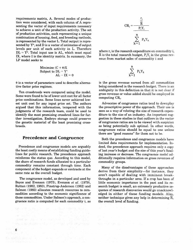
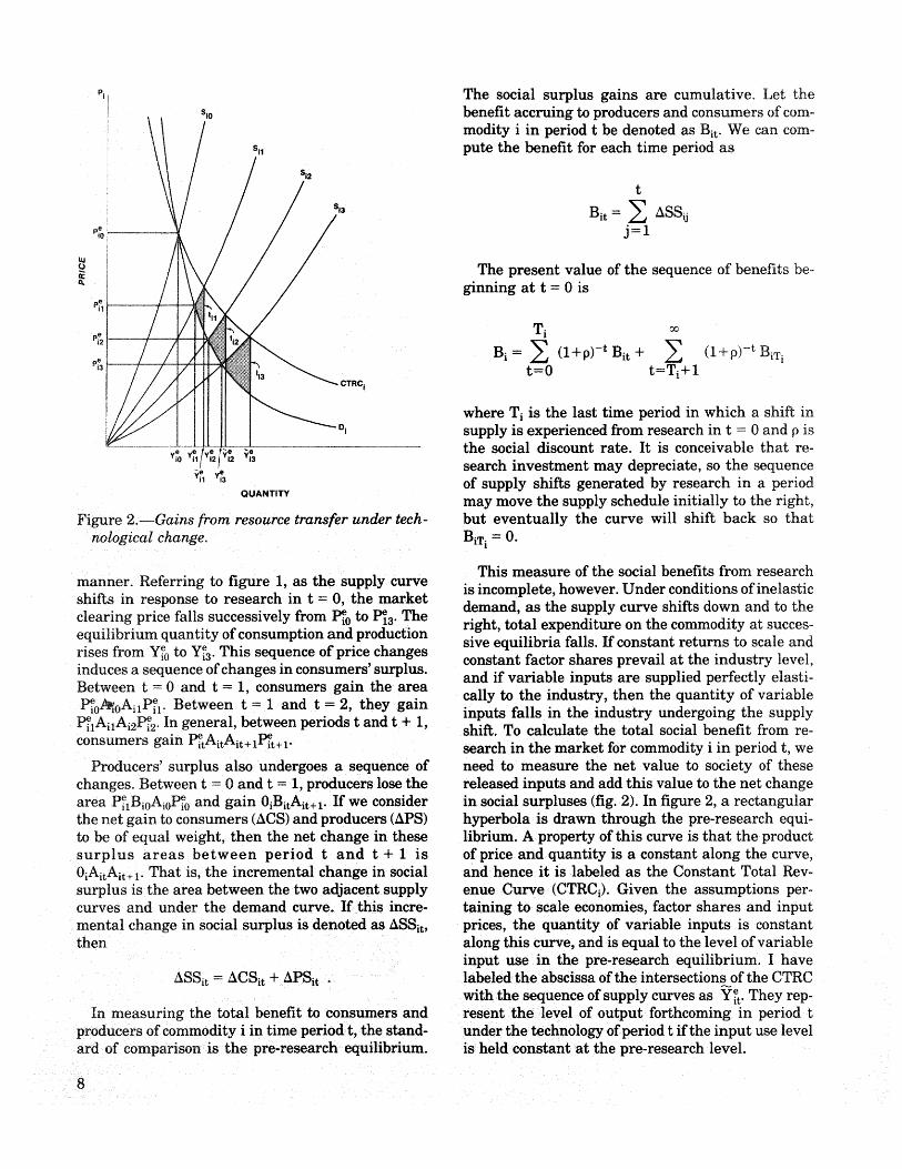
Public investment in agricultural research is modity prices change and also yield resource savingsmade over a protracted period, and benefits occur when demand is inelastic. Figures 1 and 2 identifyafter a lag of several years. Several analysts have these gains for a sequence of supply shifts.acknowledged this fact by pursuing formal tech-niques of dynamic cost-benefit analysis to improve The demand curve in the figures is written in in-the efficiency of research resource allocation, verse form as

Net Farm Income1

Barkerand Herdt(1982)developeda modeltoal- Dlocateresearchresourcesforrice.A similarframe- PDit= % YitTMwork was advancedbyArajietal.(1978).BarkerandHerdt proposedthatresearchresourcesshouldbe whereidenotesthecommodity,trepresentstime,Pallocatedacrosstypesofricetomaximizethedis- isthepriceofcommodityipaidby consumersand Ycountedstreamsof expectedchangesin netfarm isthequantitythatwouldbe purchasedatpriceP.income(NFI)forthecommoditiesinquestion.This Thisisa constantelasticitydemand curve,where_Damounts tochoosinga vectorofresearchfunding istheelasticityofdemand forcommodityi.The fig-levels, Ro = {rio, r20, r30, . . . rno}, to maximize ures are drawn for the case -1 < vlD< 0. The situa-

tion for miD< -1 can be derived in a straightforward

n{ }* (Ro;F)= _ _ (I+p)-tA NFIit(rio,F) I$I0

i=1 t=0

Si1where p isthediscountrate,A NFIit(')denotesthe %change in aggregate net farm income for commod- Iityiinperiodt asa functionofrio,and F isa vector / %

of parameters. P_0 ///

While this criterion has a certain intuitive appeal, _ /it fails to take into account the benefits accruing to _ //consumers in the form of lower commodity prices.When an industry faces inelastic demand, net farm p_l / /income can be depressed by technological change, /and yet the net benefit to society as a whole is posi- P_= 'tive. From this perspective, the net farm income P_s /criterion will, in general, be a poor guide to the allo-cation ofresearchresources.

D

Social Surplus Criterion p_=Y_v,,"_

A surprising feature of much of the literature ad- o, v_0-,v"._=v._,v,dressing the problem of ex ante optimal research al- aUA,T_Tvlocation is that it bears little relation to the analyti-cal framework used in studies of ex post estimates of Figure 1.--Changes in consumers' and producers"gains to research. The latter studies measure the surpluses for a sequence of supply shifts.

7

P, The social surplus gains are cumulative. Let the% benefit accruing to producers and consumers of com-modity i in period t be denoted as Bit. We can corn-

s,, pute the benefit for each time period as

Si2

13 Bi t = _SSi j

P_o j= 1

u / The present value of the sequence of benefits be-ginning at t = 0 is

,, T.c _ 2

,, Ti _

P_2 _ gi = (I+P)- t Bit + (I+P)- t BiTi

P_'3 / t=0 t=Ti+ii

where T i is the last time period in which a shift insupply is experienced from research in t - 0 and p isthe social discount rate. It is conceivable that re-

v_'ov_ ,2_'2_'3 search investment may depreciate, so the sequence_1 _3 of supply shifts generated by research in a period

QUANTITY

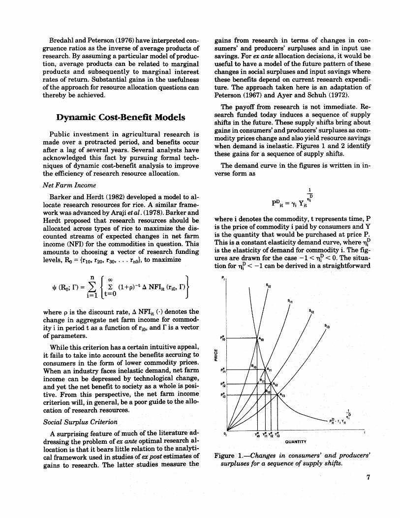
may move the supply schedule initially to the right,Figure 2.--Gains from resource transfer under tech- but eventually the curve will shift back so that

nological change. BiT i ----0.

This measure of the social benefits from research

manner. Referring to figure 1, as the supply curve is incomplete, however. Under conditions of inelasticshifts in response to research in t = 0, the market demand, as the supply curve shifts down and to theclearing price falls successively from l_i0 to P_13.The right, total expenditure on the commodity at succes-equilibrium quantity of consumption and production sive equilibria falls. If constant returns to scale andrises from Yie0to Yie3. This sequence of price changesinduces a sequence of changes in consumers' surplus, constant factor shares prevail at the industry level,and if variable inputs are supplied perfectly elasti-Between t = 0 and t = 1, consumers gain the area cally to the industry, then the quantity of variablee . e

Pio/_ioAilPil. Between t = 1 and t = 2, they gain inputs falls in the industry undergoing the supplypea ^ De In general, between periods t and t + 1,

ilFXilZ'Xi2_i2" shift. To calculate the total social benefit from re-

consumers gain P_itAitAit+ 1Piet+l . search in the market for commodity i in period t, weProducers' surplus also undergoes a sequence of need to measure the net value to society of these

changes. Between t = 0 and t = 1, producers lose the released inputs and add this value to the net changearea PelBioAi0Wioand gain 0iBitAit+l . If we consider in social surpluses (fig. 2). In figure 2, a rectangularthe net gain to consumers (hCS) and producers (APS) hyperbola is drawn through the pre-research equi-to be of equal weight, then the net change in these librium. A property of this curve is that the productsurplus areas between period t and t + 1 is of price and quantity is a constant along the curve,0iAitAit+ 1- That is, the incremental change in social and hence it is labeled as the Constant Total Rev-surplus is the area between the two adjacent supply enue Curve (CTRCi). Given the assumptions per-curves and under the demand curve. If this incre- taining to scale economies, factor shares and inputmental change in social surplus is denoted as ASSit , prices, the quantity of variable inputs is constantthen along this curve, and is equal to the level of variable

input use in the pre-research equilibrium. I have_SSit _- _CSit + APSit . labeled the abscissa of the intersections of the CTRC

with the sequence of supply curves as Yiet. They rep-In measuring the total benefit to consumers and resent the level of output forthcoming in period t

producers of commodity i in time period t, the stand- under the technology of period t if the input use levelard of comparison is the pre-research equilibrium, is held constant at the pre-research level.

8

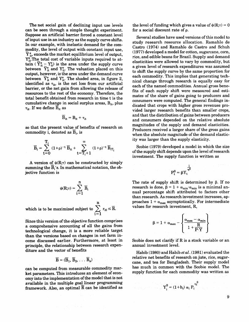
The net socialgainofdeclininginputuselevels theleveloffundingwhichgivesa valueof,(R;v)= 0can be seenthrougha simplethoughtexperiment, fora socialdiscountrateofp.Supposean artificialbarrierforceda constantlevel Severalstudieshaveusedversionsofthismodelto

ofinputuseinan industryasthesupplycurveshifts, studyresearchresourceallocation.Ramahlo deInourexample,withinelasticdemand forthecom- Castro(1974)and Ramahlo de Castroand Schuhmodity,thelevelofoutputwithconstantinputuse, (1977)developedamodelforcotton,sugarcane,corn,y e exceedsthemarketequilibriumlevelofoutput,it, rice,and ediblebeansforBrazil.Supplyanddemand

Yet.Thetotalcostofvariableinputsrequiredtoat- elasticitieswereallowedtovaryby commodity,butthin(Yiet-Yiet)isthe areaunderthesupplycurvebetween Yietand Yiet.The valuationplacedon this a givenlevelofresearchexpenditureswas assumed

toshiftthesupplycurvebythesame proportionforoutput,however,istheareaunderthedemand curve eachcommodity.Thisimpliesthatgeneratingtech-between Yietand Yiet.The shadedarea,infigure2, nicalchangethroughresearchisequallyeasyforidentifiedas "tit,isthe net lossfrom our artificial eachofthenamed commodities.Annual grossbene-barrier,orthenetgainfromallowingthereleaseof fitsofeach supplyshiftwere measured and esti-resourcestotherestoftheeconomy.Therefore,thetotalbenefitobtainedfromresearchintimetisthe matesoftheshareofgainsgoingtoproducersand

consumerswerecomputed.The generalfindingsin-cumulativechangeinsocialsurplusareas,Bit,plus dicatedthatcropswith highergrossrevenuespro-Tit.Ifwe defineBit as videdlargerresearchbenefitsthan smallercrops,

-- and that the distribution of gains between producersBit- Bit %Tit and consumers depended on the relative absolute

magnitudes of the supply and demand elasticities.so that the present value__ofbenefits of research on Producers received a larger share of the gross gainscommodity i, denoted as Bi, is when the absolute magnitude of the demand elastic-

Ti cc ity was larger than the supply elasticity.

Si -" _ (l+p)-tBit "{- _ (1+p)-t_iTi Scobie (1979)developeda modelinwhichthesizet= 0 t=Ti+1 ofthesupplyshiftdependsuponthelevelofresearch

investment.The supplyfunctioniswrittenas

A versionof,(R;v)canbe constructedby simply±

summing the Bi's. In mathematical notation, the ob- msjective function is pS = _Yt

n The rate of supply shift is determined by 6. If no

$(R;T) = _ Si research is done, _ = 1 + Otmin'O_min is a minimal an-i=l nual percentage shift attributed to factors other

than research. As research investment increases, ap-n proaches 1 + ama_ asymptotically. For intermediate

which is to be maximized subject to _ rio -values for research investment, R,

Sincethisversionoftheobjectivefunctioncomprises _ = I + amax-- Otmax-- OLmin

a comprehensiveaccountingofallthe gainsfrom Rtechnologicalchange,itisa more reliabletargetthantheversionsbasedon changesinnetfarm in-come discussedearlier.Furthermore,at leastin ScobiedoesnotclarifyifR isa stockvariableoranprinciple,therelationshipbetweenresearchexpen- annualinvestmentlevel.

ditureand thevectorofbenefits Habib(1980)andHabibetal.(1981)evaluatedthe-- relative net benefits of research on jute, rice, sugar-

B = (B1, B2, • • • Bn) cane, and tea for Bangladesh. Their supply model

can be computed from measurable commodity mar- has much in common with the Scobie model. Theket parameters. This introduces an element of econ- supply function for each commodity was written asomy into the implementation of the model that is not

Savailable in the multiple goallinear programming _i

y.S (l+hi)aiPiframework. Also, an optimal R can be identified as , =

9

The h i term represents a percentage shift in the sup- spillover models represents the contribution of re-ply function in response to research. The size of the search as a shift variable in the production or supplyshift is a linear function of the research investment, function. In the Ziemer et al. (1982) study, the sup-so that ply function for aggregate agricultural output in a

region i is represented as

h i = Si Ri

up to a maximum possible shift of hu. It is not made _is 1-8 _-_clear if R is an annual investment level or a stock Yit = cqPit Yit_l i exp 8i gij+git

concept. Values for the S's were obtained by compar- [_ j =0ing crop yields in Bangladesh with yields elsewhere

in Asia. The study concluded that potential gains The shift function, exp {.} reflects the effects of re-from research were highest for rice and then for search inside and outside of the region through thesugarcane, formula that determines the git'S. The effect of re-

All of the models discussed in this section make search on output was estimated using an adaptation

important strides in conceptualizing the research of the technique introduced by Cline (1975). A multi-budgeting process as an optimization problem. They factor productivity index (PR) for each region wasalso highlight some critical data requirements regressed on lagged research inside (RI) and outsidewhich were ignored in the models of earlier sections. (RO) of the region, the level of farmers' education inThe magnitudes of supply and demand elasticities, the region (E) and a weather index (W). The func-the functional forms of these schedules, the mecha- tional form employed wasnism by which research investment shifts supply allreceive a deserved emphasis. All of this, however, 13 13

tends to show that these models are more costly to PRit = H Ro]_J-j [-] RI_J-j E_ exp {5oi+ _li Wit}estimate and use than the precedence or congruence j =0 j-_)'=approaches, but are likely to be less costly than theuse of scoring models. Furthermore, reliance on the The value of the a's and the B's were then used tonotions of consumers' and producers' surpluses compute the g functions, according tomakes these models vulnerable to all of the theoret-

ical arguments that undermine the credibility of 10

those measures of economic welfare (Chipman and EMoore 1976, 1980; McKenzie 1982). git = 0.10 oqtS i + 1/(1-Ri) 0.10 _itSjl_j=lj4:l

Models of Regional Spillover S k represents the share, in value terms, of nationalEffects crop and livestock output originating in region k. R

is the regional percentage of research expenditure asLessons learned from agricultural research in one a share of the national total. The 0.10 coefficient

region can often be adapted and applied in another indicates that the analysis was conducted to considerregion with similar agro-climatic characteristics, a hypothetical 10 percent increase in research ex-These spillover effects have important consequences penditure. Weighting the contribution of other re-for optimal public financing of regional research cen- gions research by (1 - Ri)-1 means that a regionters by a federal government. Simply put, a region which has a high value for Ri would benefit morewhich generates large spillover benefits should re- from spill-ins than a region with a lower level ofceive a commensurately higher level of federal fund- internal research investment.ing than a region which doesn't generate this effect. The findings of this set of studies indicate thatSeveral economists, including Garren and White federal research funding in the United States has(1981), Garren (1981), Ziemer et al. (1982), White not reflected regional patterns of benefit transmis-and Havlicek (1981), and Havlicek and White (1983)have recently turned their attention to this regional sion. A realignment of funds to increase research in

regions generating large spillovers was recom-allocation question for the case of the U.S. economy, mended. None of the papers cited above, however,

As with the dynamic cost-benefit models, the ana- took the final step of computing an optimal regionallytical framework employed in these regional allocation pattern.

i0

The analytical framework employed in these re- a constant growth rate of the total labor forcegional studies is essentially the same as that in thecost-benefit models outlined above, and is subject to L(t)/L(t) = nthe same information requirements and theoreticallimitations. Additional care was taken in the re- Output is allocated between consumption, C(t), andgional models to identify the time lag structure of gross investment, I(t)research benefits, and this is an important contribu-tion. I(t) + C(t) -<Y(t)

Optimal Growth Models 2 at each moment of time, and the capital stock, K(t),evolves according to

The study of optimal economic growth has tradi- I4(t) = I(t) - 5K(t)tionally been the province of development special-

ists, macroeconomists, and theorists. More recently, A constant rate of depreciation is represented by 8.resource and agricultural economists have begun toapply this approach to the study of technological These constraints are imposed on the objectivechange. Optimal growth models have typically been function, which seeks to maximize the discountedused to study resource allocation at the national or stream of consumption per caput. The problem is setsectorial level, but some less aggregate efforts have up for an infinite horizon and with a constant rate ofbeen undertaken, social time preference, p.

One of the earliest applications of control theory to Thustechnical change was made by Uzawa (1965). In hismodel, the allocation decision focuses on dividing the ctotal labor force at time t, L(t), between employment | [c(t)/L(t)]e -ot dtin production, Lp(t), and employment in the educa- J0

tional or research sector, Le(t). The production func-tion is represented as: Functional forms for the production function and

the technology index are not specified, so a quantita-Y(t) = F [K(t), T(t) Lp(t)] tive solution to the model is found. It is useful to

develop some additional notation. The effectivewhere T(t) is an index of labor efficiency. This index capital-labor ratio is defined asincreases as a larger share of the labor force is em-ployed in the research sector. Research workers pro- x(t) = K(t)/[T(t).L(t)]duce knowledge that makes production workersmore effective. The movement of T(t) through time is The savings ratio is defined asgoverned by

s(t) = I(t)/Y(t)

q?(t)/T(t) = 0 [Le(t)/L(t)] = 0 [1-u(t)]The optimal solution obtained is a balanced state

where u(t) = Lp(t)/L(t). q?(t)/T(t) denotes the growth described by the time paths of u(t), x(t) and s(t). Letrate of T(t). It is assumed that increasing the share a superscript* denote the value of a variable in itsof the labor force employed in research increases the optimal state. If, by coincidence, the initial effectiverate of growth of T(t), so that 0' ->0. This effect is capital-labor ratio is optimal, that issubject to decreasing returns, however, so 0" -<0.

x(0) = xOther assumptions in the model include full em-

ployment of a finite labor force at each moment of then optimal growth is achieved by choosing a sav-time, ings rate and an allocation of the labor force so that

the technology index increases at the same rate asLp(t) + Le(t) = L(t) the capital labor ratio. Mathematically,

2Readers unfamiliar with the techniques of control ._?(t)fr(t) = l_(t)/k(t) ,theory are referred to Intrilligator (1971), Takayama(1974), and Kamien and Schwartz (1981). where k(t) = K(t)/L(t).

11

\

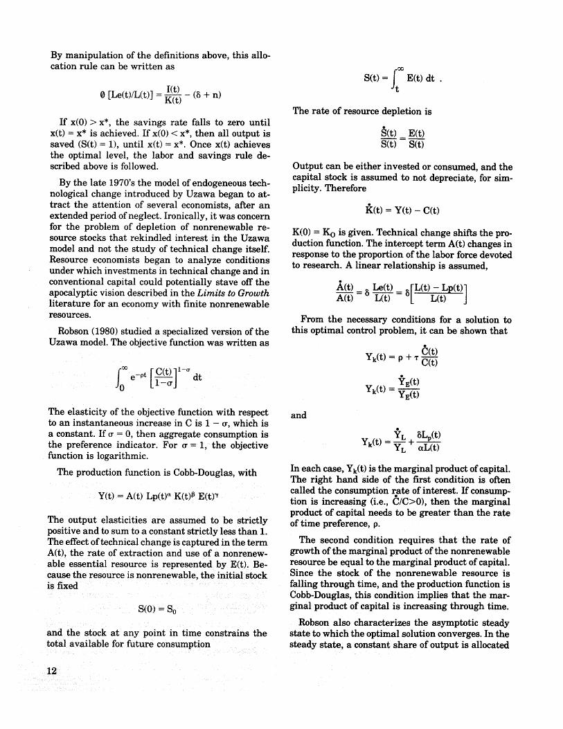
By manipulation of the definitions above, this allo-cation rule can be written as

P O0

S(t) = | E(t) dt o

I(t) Jt0 [Le(t)/L(t)] - K(t---)- (8 + n)

The rate of resource depletion isIf x(0)> x*, the savings rate falls to zero until

x(t) = x* is achieved. If x(0) < x*, then all output is S(t) = E(t)saved (S(t)= 1), until x(t)= x*. Once x(t) achieves S(t) S(t)the optimal level, the labor and savings rule de-scribed above is followed. Output can be either invested or consumed, and the

capital stock is assumed to not depreciate, for sim-By the late 1970's the model of endogeneous tech- plicity. Therefore

nological change introduced by Uzawa began to at-

tract the attention of several economists, after an I_(t) = Y(t)- C(t)extended period of neglect. Ironically, it was concern

for the problem of depletion of nonrenewable re- K(0) = Ko is given. Technical change shifts the pro-source stocks that rekindled interest in the Uzawa duction function. The intercept term A(t) changes inmodel and not the study of technical change itself.

response to the proportion of the labor force devotedResource economists began to analyze conditions to research. A linear relationship is assumed,under which investments in technical change and in

conventional capital could potentially stave off the ,_(t) = 8 Le(t)[L(t)_tLp(t) ]apocalyptic vision described in the Limits to Growth A(t) _ = 8literature for an economy with finite nonrenewable

resources. From the necessary conditions for a solution toRobson (1980) studied a specialized version of the this optimal control problem, it can be shown that

Uzawa model. The objective function was written as C(t)Yk(t) = P + • C(t)

oo

f0 e_Pt [C(t)]l-a[l_--Z_j dt Yz(t)Yk(t) = YE(t)

The elasticity of the objective function with respect andto an instantaneous increase in C is 1 - _, which is

a constant. If a = 0, then aggregate consumption is YL 8Lp(t)the preference indicator. For _ = 1, the objective Yk(t) =_LL + aL(t)function is logarithmic.

In each case, Yk(t) is the marginal product of capital.The production function is Cobb-Douglas, withThe right hand side of the first condition is oftencalled the consumption rate of interest. If consump-

Y(t) = A(t) Lp(t) _ K(t)_ E(tP tion is increasing (i.e., C/C>0), then the marginalproduct of capital needs to be greater than the rate

The output elasticities are assumed to be strictly of time preference, p.positive and to sum to a constant strictly less than 1.The effect of technical change is captured in the term The second condition requires that the rate ofA(t), the rate of extraction and use of a nonrenew- growth of the marginal product of the nonrenewableable essential resource is represented by E(t). Be- resource be equal to the marginal product of capital.cause the resource is nonrenewable, the initial stock Since the stock of the nonrenewable resource isis fixed falling through time, and the production function is

Cobb-Douglas, this condition implies that the mar-

S(0) = So ginal product of capital is increasing through time.

Robson also characterizes the asymptotic steadyand the stock at any point in time constrains the state to which the optimal solution converges. In thetotal available for future consumption steady state, a constant share of output is allocated

12

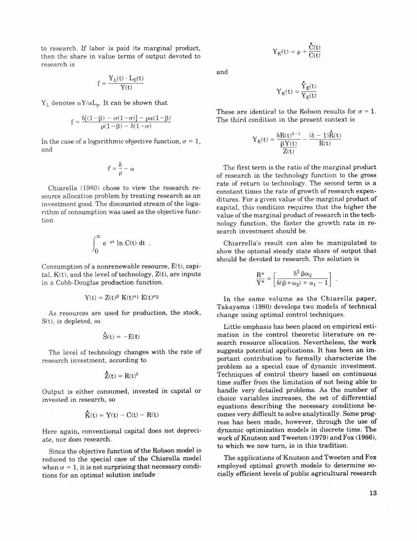
to research_ If labor is paid its marginal product, YK(t) = P + Cit)then the share in value terms of output devoted toresearch is

andYh(t) - L¢(t)

f =

Y(t) Y_(t)....Y#t)

YL denotes{_YA_Lp.Itcan be shown thatSFhe_ e are identical to the Robson results for (7 = 1.

f = _l,L_-)\ °TS(1-_r)_. - ) The third condition in the present context is

5R(t) _--_ (8 ......i)[(t)

tn the case of a logarithmic objective function, {:r....1, YK(t) .... _Y{ t) R{t)and Z(t)

f 8..... c_ The first term is the ratio of the marshal plx)ductP of research in the technology function to the gross

rate of return to technology. The second term is aChiarella (1980).chose to view the research re-

constant times the rate of growth of research expen-source allocation problem by treating research as an ditures. For a given value of the marginal product ofinvestment good. The discounted stream of the loga- eapitak this condition requires that the higher therithm of consumption was used as the objective fhnc- value of the marginal product of research in the tech-tion nology function, the faster the grouch rate in re-

search investment should be.

e -_ In C(t)dt Chiarretla's result also be manipulated tocan

-0 show the optimal steady state share of output thatshould be devoted to research. The solution is

Consumption of a nonrenewable resource, E(t), capi-

tal, K(t), .and the level of technology, Z{t), are inputs [_! = [ _ [_2 }in a Cobb-Douglas production function. Y* [8(_+a2 t + _l - 1

Y(t) = Z(t) _ K{t) '_l Eft) _2 in the same volume as the Chiarelta paper,Takayama (1980) develops two models of technical

As resources are used for production, the stock, change using optimal control techniques.S.t), is depleted, so

Little emphasis has been placed on empirical esti-

S(tl =-E(t) marion in the control, theoretic literature on re-search resource allocation. Nevertheless, the work

The level of technology changes with the rate of suggests potential applications. It has been an im-research investment, according to portant contribution to formally characterize the

problem as a special case of dynamic investment.

Ztt) = R(t) _ Techniques of control theory based on continuoustime suffer t_om the limitation of not being able to

Output is either consumed, invested in capital or handle very, detailed :problems. As the number ofinvested in research, so choice variables increases, the set o:f differential

equations describing the necessary conditions be-* tK(1) = Y(t) - C(t) R(t) comes very difficult to solve analytically. Some prog-

ress has been made. however, through the use of

Here again, conventional capital does not depreci- dynamic optimization models in discrete time, Thea_, nor does research, work of Knutson and Tweeten t 1..979)and Fox .(1986),

to which we now turn..is in this tradition.Since the objective function of the Pvjbso:n model is

reduced to the special ease of the Chiarella model The applications of Knutson and Tweeten and Foxwhen _:_= 1, it is not surprising that necessary condi- employed optimal growth models to determine so-tions fbr an optimal solution include cially efficient levels of public agricultural research

13

for the U.S. farm sector. Knutson and Tweeten con- evidence of underinvestment in agricultural re-sidered the farm production sector as a unit. Fox's search, but the solution of the Fox model indicatedmodel had separate livestock and crop sectors. Both that optimal funding for each of the categories ofstudies used a revised version of Cline's model of the research was on the order of four times the actualproduction function for agriculture. The Knutson level in the late 1970's. The aggregate underinvest-and Tweeten study considered three scenarios for ment problem was found to be equally serious forreal increases in funding: each of the four research types. Neither crops nor

1. Expenditures would grow in real terms by livestock research or basic nor applied research wasfound to be relatively more inadequately supported.3 percent per year from 1976-2015, which rep-

resents an extrapolation of the trend from1939-1972.

2. Real funding growth of 10 percent per year for IDENTIFYING SOUTHERN PINE1976-1980, followed by 3 percent real growth FORESTRY RESEARCH PRIORITIESto 2015.

3. Ten percent growth from 1976-1980 followed Backgroundby 7 percent growth annually to 2015.

The effect of these research investments on output The southern pine forestry research effort has re-prices and production levels was estimated with the cently become a focus of attention, due in part to theNational-Interregional Projections system (Yeh Southern Timber Study. The USDA Forest Service1976) for various assumptions about the rate of has brought together the diverse forestry interestgrowth in demand for farm products. Social rates of groups in the South in an effort to develop an analyt-return to research investments were computed for ical database for formulating and guiding public andeach of the funding and demand growth combina- private forest policies. It is possible to apply tech-tions. Research investment was considered socially niques discussed earlier to southern pine forestry toprofitable if the rate of return was not depressed determine research priorities.below 10 percent. If demand growth was held to 1.2

The research resource allocation question con-percent per annum, then the historical rate of in-

cerns the choice of funding levels for types of forestrycrease in funding was found to be consistent with the

research for essentially a single output. Categoriesoptimality criterion. This would lead to a doubling of include fire, insect, disease 3, renewable resourceannual support for research by the end of the cen-tury. Higher rates of research funding were optimal evaluation, renewable resource economics, timber

management, forest products utilization, forestryfor higher levels of demand growth. The effect of engineering and other4. The last three categories areexport market behavior on demand growth was not predominantly concerned with post-harvest re-reported, search problems. The focus of this study is on the

The Fox study used a three sector growth model, allocation of research resources for pre-harvestLivestock production, crop production, and the rest forestry problems.of the economy were represented. The model sought

to maximize the discounted stream of the logarithms Congruence CalcuLationsof annual consumption of output of the three sectors

weighted by shares of annual consumption expendi- While congruence ratios possess limited prescrip-ture. The objective function was constrained by pro- tive power, the approach does give some insight intoduction functions for each sector and by factor en- the intensity of research investment across commod-dowrnents. Crops could be exported in exchange for ity groups and regions. Tables 4 and 5 document thegoods which substituted for the output of the non- level of Federal research funding in the South. Vol-farm sector. Four categories of research were identi- ume and value of production are reported in table 6.fled. "Basic", or non-commodity specific biologicalresearch, and "applied", a commodity specific re-search aimed at the farm production sector, were

identified for each of the two farm sectors. These 3As of 1974, the insect and disease categories werepublic investment variables competed with con- reported as a combined total.sumption and with conventional capital investment 4Includes cooperative aid, insect and disease con-inside and outside of agriculture, trol detection and appraisal, range, recreation, re-

The findings of this report contrasted with the re ........... and supply, research construction, water-sults of the Knutson and Tweeten study. Both found shed, wildlife and fish habitat, and miscellaneous.

14

Similar tables could be constructed for the other re- A Social Surplus Model of Researchin the United States and sets of congruencecould be formulated. Comparisons could be Resource Allocation

of functional activity categories of research perof product value across regions. Using the Data on inputs up to the point of harvest are quiteForest Service Wildfire Statistics, compari- limited, which precludes the use of a production

could be made of the levels of fire prevention function model. It is possible, however, to develop acontrol research relative to the actual incidence social surplus model along the lines of those pre-

across regions, sented earlier. A model of supply and demand areneeded. A log-linear version of the demand function

should be noted that tables 4 and 5 report Fed- could be estimated asresearch allocations. If it is suspected that State

allocations among functional activities vary among lnYtD= _D + _IDIn Pt + .ql In Itregions, similar tables for State expenditures would

necessary to complete the congruence picture.

Table 4.--Federal research funds allocated to the Southern ForestExper_-----_merlt Station by_ n__n-_-_ac tivity, i955-1983

(In current dollars)

Fu-6ctionalactfvTt-_Year _a-b-l-e .... -Re-n-ewabIe

resource resource Timber

Fire Insect Disease evaluation economics management

1955 8,500 31,200 32,750 105,000 12,000 341,8461956 8,500 49,624 32,750 105,000 12,000 544,513i957 36,786 65,000 52,000 136,000 42,i00 686,000i958 38,276 68,058 54,145 176,565 44,956 767,4401959 38,276 68,054 54,145 176,529 44,956 986,3811960 40,496 72,613 57,725 185,813 47,9i6 1,044,830i961 50,791 88,175 73,133 187,253 48,224 1,161,315i962 78,091 147,975 152,633 219,903 80,924 1,348,965i963 78,091 168,975 166,633 217,903 80,924 1,339,9651964 82,691 205,095 178,233 231,703 86,i24 1,538,7451965 84,070 425,355 215,510 264,640 87,740 1,583,910i966 85,550 432,605 220,500 270,390 89,800 1,649,7901967 87,850 472,305 253,500 296,090 99,030 1,683,7591968 89,900 601,200 268,000 328,600 140,100 1,786,8001969 91,900 621,200 276,800 339,700 144,800 i ,847,400i970 111,700 639,600 285,300 381,400 151,200 1,924,100197i 115,700 683,600 331,300 490,400 207,200 2,081,1001972 123,100 749,700 510,800 536,400 228,100 2,248,2001973 123,500 888,000 476,200 538, i00 228,900 2,770,6001974 123,500 1,400,200 538, i00 228,900 2,347,6001975 134,100 1,521,100 588,400 252,300 2,669,9001976 138,300 2,063,400 710,300 265,200 2,671,5001977 145,900 2,262,200 1,059,000 284,900 2,871,9001978 152,700 2,371,200 1,445,000 301,300 3,556,i001979 159,000 2,532,000 1,485,000 3i3,000 4,211,0001980 103,000 2,650,000 1,511,000 321,000 4,361,0001981 174,000 3,607,000 i, 716,000 389,000 5,196,0001982 155,000 3,516,000 1,572,000 394,000 4,621,000i983 3,506,U00 1,673,000 385,000 4,60i,000

15

Table 5.--Federal research funds allocated to the Southeastern Forest ExperimentStation by functional actT_. i955-1983

(In current dollars)

Func ti on-al ac tiv i tyYear Renewable Renewal)l e

resource resource Timber

Fire Insect Disease evaluation economics management

1955 25,477 30,714 62,158 90,000 14,500 320,040i956 25,477 30,714 62,(900 90,000 15,000 430,1981957 40,112 45,L}O0 68,000 120,000 42,000 454,0001958 132,033 47,908 82,900 164,500 43,500 510,1961959 202,U83 47,909 82,900 164,500 43,500 643,526i960 213,859 51,731 87,774 173,145 46,374 691,9971961 214,732 76,917 1i2,780 173,640 46,651 739,5121962 275,032 132,417 214,980 202,459 74,051 848,3121963 278,032 163,066 269,246 200,459 85,701 770,8371964 294,432 270,265 345,946 213,159 91,101 818,0371965 299,360 423,880 425,750 240,740 92,800 925,0601966 458,950 458,770 434,850 247,560 94,450 949,5101967 459,350 502,270 453,550 283,340 152,920 1,089,6411968 469,800 514,700 469,400 313,500 162,600 1,169,700i969 463,800 533,300 486,500 324,800 168,I00 1,255,300i970 479,900 549,500 528,900 356,900 171,600 1,292,3001971 508,900 586,500 525,900 426,900 181,600 1,406,300i972 569,600 645,700 575,100 465,800 197,900 1,707,900i973 1,097,800 648,500 577,200 467,400 198,600 1,720,300i974 917,800 1,225,700 467,400 198,600 1,791,9001975 978,500 1,330,700 516,100 184,200 1,971,4001976 1,122,300 1,907,900 630,200 193,200 2,367,800i977 1,201,600 2,000,900 973,900 207,000 2,524,0001978 1,251,100 2,071,200 1,328,300 215,700 3,013,6001979 1,297,000 2,067,000 1,380,000 222,000 3,188,0001980 1,364,000 2,i03,000 1,430,000 253,000 3,066,0001981 1,459,U00 2,303,000 1,656,000 384,000 3,699,0001982 1,276,000 1,990,000 1,407,000 330,000 3,285,U001983 £,257,000 2,i79,000 1,614,000 343,000 3,095,000

where YtDis the level of production from table 6, Pt constant elasticity log-linear supply schedule couldthe stumpage price of table 6 suitably adjusted for be estimated as

inflation, and I t is a measure of real national income.

and 01 are the elasticities of demand with respect / I J

priceand incomerespectively. Yts I )= _ R_ijBecausetreestaketimetomatureand canbehar- l-] I-[p_sFt (St)]t-i

i=0j=1 ,vestedat variousstagesofgrowth,supplyismoredifficulttomodel.Conceptually,we want torelate

levelofharvestactivity,Y_,to thestumpage l_t_iisthelevelofresearchexpenditureon func-price,Pt,and to laggedexpendituresofresearch, tionalactivityj intimeperiodt - i.Therearefive

To reflectthedynamicnatureoftheproduction relevantcategoriesoffunctionalactivities.Itistug-processforwood,a variablewhich is intendedto gested,basedontheagriculturalresearchliterature,approximatethestockofwood,St,isalsoincluded.A that a quadratic distributedlag with zero-

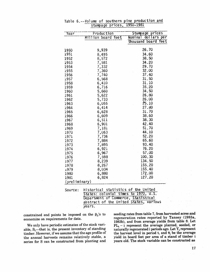
Table 6.--Volume of southern pine production andstumpage prices, 1950-1981

-Year Pro_tion Stumpage pricesM_oard feet Nominal dollars per

thousand board feet

1950 9,939 26.70i951 8,495 34.601952 8,572 38.50i953 7,581 34.201954 7,332 29.70i955 7,360 32.O01956 7,740 37.40i957 6,568 31.501958 6,410 31.101959 6,716 35.201960 5,660 34.501961 5,622 26.801962 5,733 26.O01963 6,055 L_5.101964 6,414 27.801965 6,628 31.701966 6,609 38.601967 6,511 38.301968 6,901 42.40i969 7,18i 51.701970 7,063 44.101971 7,736 52.201972 7,884 65.601973 7,895 93.401974 6,92i 76.201975 6,967 57.001976 7,598 100.301977 8,239 134.501978 8,267 155.201979 8,034 155.401980 6,880 172.O01981 6,824 127.20(preliminary)

Source: Historical statistics of the UnitedStates: c-OlOnial times to 1970, U.S._epart_nentof Comn_rce, Statisticalabstract of the United States, variousyears.

constrained end points be imposed on the _ji'S to seeding rates from table 7, from harvested acres andeconomize on requirements for data. regeneration rates reported by Tansey (1983a,

1983b), and from average yields from table 8. LetWe only have periodic estimates of the stock vari- PLt - i represent the average planted, seeded, or

able, St--that is, the present inventory of standing naturally regenerated i periods ago. Let Yt representtimber. However, if we assume that the age profile of the harvest level in period t, and Oi be the averagethe annual harvests remains relatively stable, a yield in board feet per area of a stand of timber iseries for S can be constructed from planting and years old. The stock variable can be constructed as

17

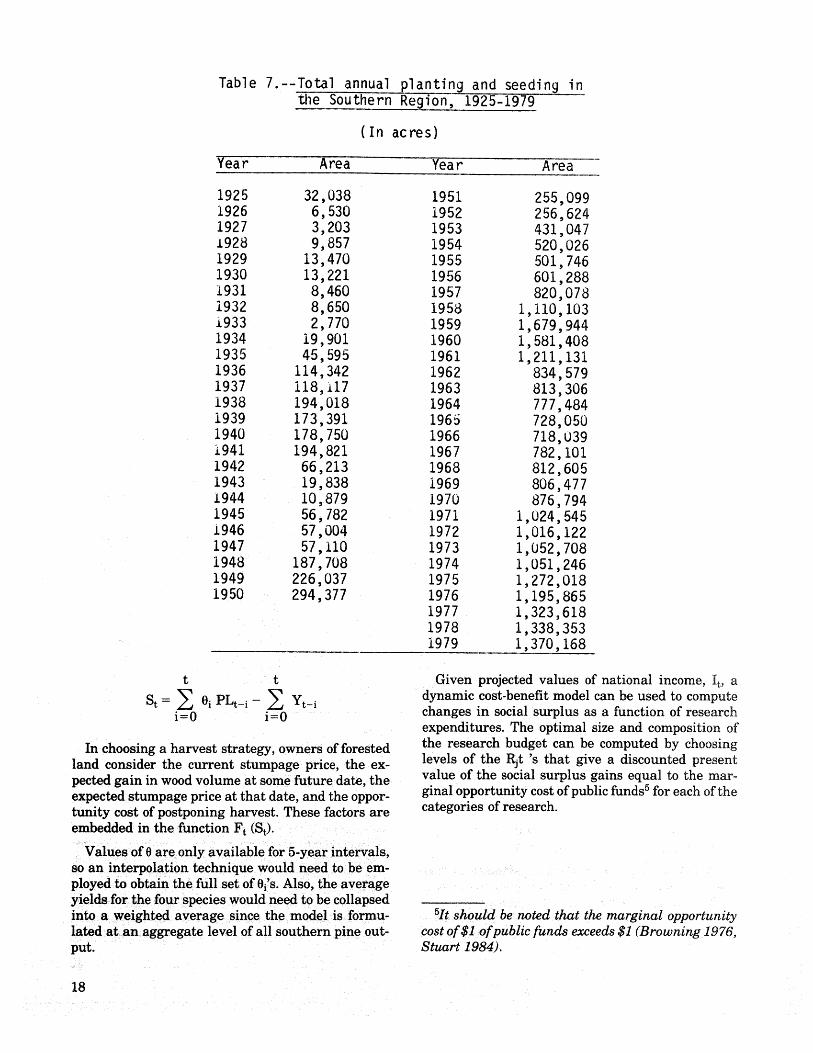
Table 7.--Total annual planting and seeding inthe Southern Region, 1925-1979

(In acres)

Year Area Year Area

1925 32,038 1951 255,0991926 6,530 i952 256,6241927 3,203 1953 431,047i928 9,857 1954 520,0261929 13,470 1955 501,7461930 13,221 1956 601,288i931 8,460 1957 820,0781932 8,650 1958 i,i10,103i933 2,770 1959 1,679,9441934 i9,901 1960 i,581,4081935 45,595 1961 1,211,13i1936 114,342 1962 834,5791937 i18,i17 1963 813,306i938 194,018 1964 777,4841939 173,391 1965 728,0501940 178,750 1966 718,U39i941 194,821 1967 782,1011942 66,213 1968 812,6051943 19,838 i969 806,477i944 10,879 1970 876,7941945 56,782 1971 i,024,545i946 57,004 1972 i,016,1221947 57,i10 1973 1,052,7081948 187,708 1974 i,051,2461949 226,037 1975 I,272,0181950 294,377 1976 1,195,865

1977 1,323,6181978 1,338,353i979 1,370,168

t t Given projected values of national income, It, a

St = _ 0i PLt-i _ Yt-i dynamic cost-benefit model can be used to computei=0 i=0 changes in social surplus as a function of research

expenditures. The optimal size and composition of

In choosing a harvest strategy, owners of forested the research budget can be computed by choosingland consider the current stumpage price, the ex- levels of the l_t's that give a discounted presentpected gain in wood volume at some future date, the value of the social surplus gains equal to the mar-

ginal opportunity cost of public funds 5 for each of theexpected stumpage price at that date, and the oppor-tunity cost of postponing harvest. These factors are categories of research.embedded in the function Ft (St).

Values of Oare only available for 5-year intervals,so an interpolation technique would need to be em-ployed to obtain the full set of Oi's.Also, the averageyields for the four species would need to be collapsedinto a weighted average since the model is formu- 5It should be noted that the marginal opportunitylated at an aggregate level of all southern pine out- cost of $1 ofpublic funds exceeds $1 (Browning 1976,put. Stuart 1984).

18

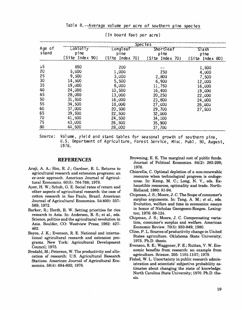
Table 8.--Average volume per acre of southern pine species

(In board feet per acre)

SpeciesAge of Loblol ly Longl-ea f Shortl eaf Slashsta nd pi ne p i ne p i ne p i ne

(Site Index 90) (Site Index 70) (Site Index 70) (Site Index 80)

i 5 850 200 --- i, 50020 5,000 i, 000 250 4,00025 9,500 3,000 2,800 7,50030 14,500 5,500 6,900 12,00035 19,000 8,000 Ii, 750 16,00040 24,000 10,500 16,400 19,00045 28,000 13,000 20,250 22,00050 31,500 16,000 23,800 24,00055 34,500 18,000 27, L)00 26,00060 37,000 20,500 29,700 27,5006 5 39,500 22,500 32,00070 41,500 24,500 34, i0075 43,000 26,500 35,90080 44,500 28,000 37,700

Source: Volume, yield and stand tables for seasonal growth of southern pine,U.S. Deparl_mnt of Agriculture, Forest Service, Misc. Publ. 50, August,i976.

I{]EF]EI{ENCES Browning, E. K. The marginal cost of public funds.Journal of Political Economics. 84(2): 283-298;

Araji, A. A.; Sim, R. J.; Gardner, R. L. Returns to 1976.agricultural research and extension programs: an Chiarella, C. Optimal depletion of a non-renewableex-ante approach. American Journal of Agricul- resource when technological progress is endoge-tural Economics. 60(5): 764-768; 1978. nous. In: Kemp, M. C.; Long, N. V., eds. Ex-

Ayer, H. W.; Schuh, G. E. Social rates of return and haustible resources, optimality and trade. North-other aspects of agricultural research: the case of Holland; 1980: 81-94.cotton research in Sao Paulo, Brazil. American Chipman, J. S.; Moore, J. C. The Scope of consumer'sJournal of Agricultural Economics. 54(400): 557- surplus arguments. In: Tang, A. M.; et al., eds.569; 1972. Evolution, welfare and time in economics: essays

Barker, R.; Herdt, R. W. Setting priorities for rice in honor of Nicholas Georgesen-Roegen. Lexing-research in Asia. In: Anderson, R. S.; et al., eds. ton; 1976: 69-124.Science, politics and the agricultural revolution in Chipman, J. S.; Moore, J. C. Compensating varia-Asia. Boulder, CO: Westview Press; 1982: 427- tion, consumer's surplus and welfare. American462. Economic Review. 70(5): 933-949; 1980.

Boyce, J. K.; Evenson, R. E. National and interna- Cline, P. L. Sources of productivity change in UnitedStates agriculture. Oklahoma State University;tional agricultural research and extension pro-

grams. New York: Agricultural Development 1975. Ph.D. thesis.Council; 1975. Evenson, R. E.; Waggoner, P. E.; Ruttan, V. W. Eco-

Bredahl, M.; Peterson, W. The productivity and allo- nomic benefits from research: an example fromcation of research: U.S. Agricultural Research agriculture. Science. 205: 1101-1107; 1979.Stations. American Journal of Agricultural Eco- Fishel, W. L. Uncertainty in public research admin-nomics. 58(4): 684-692; 1976. istration and scientists' subjective probability es-

timates about changing the state of knowledge.North Carolina State University; 1970. Ph.D. the-sis.

19

Fishel, W. L. Resource allocation in agricultural re- extension. American Journal of Agricultural Eco-search. Minneapolis: University of Minnesota nomics. 61(1): 70-76; 1979.

Press; 1971. McKenzie, G. W. Measuring economic welfare: new

Fox, G. Underinvestment, myopia and commodity methods. Cambridge University Press; 1982.bias: a test of three propositions of inefficiency in Moore, J. R.; Baker, N. R. Computational analysis ofthe U.S. agricultural research system. Canada: scoring models for R and D project selection. Man-University of Guelph, Department of Agricultural agement Science. 16(4): B-212-B-232; 1969.Economics and Business; February 1986. (mimeo) Paulson, A.; Kaldor, D. R. Evaluation and planning

Garren, N. M. The efficient allocation of agricultural of research in the experiment station. Americanresearch investment with externality consider- Journal of Agricultural Economics. 50(5): 1149-

ations. University of Georgia; 1981. Ph.D. thesis. 1160; 1968.Garren, N. M.; White, F. C. An analytical frame- Peterson, W. L. Return to poultry research in the

work for the efficient allocation of agricultural re- United States. Journal of Farm Economics. 49(3):

search expenditures by states. Agriculture Ad- 656-669; 1967.ministration. 8(4): 279-287; 1981. Pinstrup-Anderson, P. Agricultural research and

Grieg, I. D. Research management: a probabilistic ex technology in economic development. New York:ante evaluation of two broiler research proposals. Longman; 1982.Agric. Econ. Bull. 23. Armidale, NSW, Australia: Ramahlo de Castro, J. P. An economic model forUniversity of New England, Department of Agri- establishing priorities for agricultural researchcultural Economics and Business Management; and a test for the Brazilian Economy. Purdue Uni-1979. versity; 1974. Ph.D. thesis.

Habib, M. A. Optimal research, induced innovation Ramahlo de Castro, J. P.; Schuh, G. E. An empiricaland agricultural development: an application to test of an economic model for establishing re-Bangladesh. McMaster University; 1980. Ph.D. search priorities: a Brazil case study. In: Arndt,thesis. T.M.; et al., eds. Resource allocation and produc-

Habib, M. A.; Butterfield, D.; Mestelman, S. An ex tivity in national and international agriculturalante model for the allocation of research expendi- research. Minneapolis: University of Minnesotature among competing crops. Working Pap. 81-09. Press; 1977: 498-525.McMaster University, Economics Department; Robson, A. J. Costly innovation and natural re-1981. sources. International Economic Review. 21(1):

Havlicek, J., Jr.; White, F. C. Inter-regional transfer 17-30; 1980.of agricultural research results: the case of the Russell, D. G. An investigation into the use of math-Northeast. Journal of the Northeastern Agricul- ematical models for resource allocation in agricul-tural Economics Council. 12(2): 19-30; 1983. tural research. Scotland: University of Stirling;

Hildreth, R. J. Issues and implications in current 1973. Ph.D. thesis.procedures for establishing research priorities. Russell, D. G. Resource allocation in agriculturalJournal of Farm Economics. 48(5): 1641-1650; research using socio-economic evaluation and1966. mathematical models. Canadian Journal of Agri-

Intrilligator, M. D. Mathematical optimization and cultural Economics. 23(2): 29-52; 1975.economic theory. Prentice-Hall; 1971. Ruttan, V. W. Agricultural research policy. Min-

Kaldor, D. R. A framework for establishing research neapolis: University of Minnesota Press; 1982.priorities. Journal of Farm Economics. 48(5): Ruttan, V. W. Agricultural research policy issues.1629-1637; 1966. Horticulture Science. 108(6): 809-818; 1983.

Kamien, M. I.; Schwartz, N. L. Dynamic optimiza- Salmon, D. C. Congruence of agricultural researchtion: the calculus of variations and optimal control in Indonesia 1974-1978. Bull. 83-1. Minneapolis:in economics and management. North-Holland; University of Minnesota, Economic Development1981. Center; 1983.

Klein, K. K.; Kehrberg, E. W. The use of an innova- Scobie, G. M. Investment in international agricul-tion possibilities frontier to evaluate an applied tural research: some economic dimensions. Worldanimal breeding research project. Canadian Jour- Bank Staff Working Paper. 361; 1979.nal of Agricultural Economics. 29(2): 141-158; Shumway, C. R.; McCracken, R. J. Use of scoring1981. models in evaluating research programs. Ameri-

Knutson, M.; Tweeten, L. G. Toward an optimal rate can Journal of Agricultural Economics. 57(4): 714-of growth in agricultural production research and 718; 1975.

2O

Stuart,C.Welfarecostsperdollarofadditionaltax the Associationof StateUniversitiesand LandrevenueintheUnitedStates.AmericanEconomic GrantCollegesand theU.S.DepartmentofAgri-Review.74(3):352-362;1984. culture,October;1966.

Takayama, A. Mathematicaleconomics.Dryden Uzawa,H. Optimaltechnicalchangeinan aggrega-Press;1974. tivemodelofeconomicgrowth.InternationalEco-

Takayama, A. Optimaltechnicalprogresswithex- nomicReview.6(1):18-31;1965.haustableresources.In:Kemp, M. C.;Long,N.V., White,F.C.;Havlicek,J.,Jr.Interregionalspillovereds.Exhaustableresources,optimalityand trade, ofagriculturalresearchresultsand intergovern-North-Holland;1980:95-110. mentalfinance:some preliminaryresults.In:Nor-

Tansey,J.B.The pineresourceinSouthCarolina: ton,G. W. etal.,eds.Evaluationofagriculturalan interimassessment,1983.Res.Pap.SE-244. research.Misc.Publ.8-1981.St.Paul:UniversityAsheville,NC: U.S.DepartmentofAgriculture, of Minnesota,MinnesotaAgriculturalExperi-ForestService,SoutheasternForestExperiment ment Station;1981:60-70.Station;1983a. Yeh, C.J.Prices,farm outputsand incomeprojec-

Tansey,J. B. Foreststatisticsforthe southern tionsunderalternativedemand and supplycondi-coastalplainof North Carolina,1983.Resour. tions.AmericanJournalofAgriculturalEconom-Bull.SE-72.Asheville,NC: U.S.Departmentof ics.58(4):703-711;1976.Agriculture,ForestService,SoutheasternForest Ziemer,R. F.;White,F. C.;Cline,P. L. RegionalExperimentStation;1983b. welfareand agriculturalresearchand extension

U.S.DepartmentofAgriculture.A nationalprogram intheU.S.AgriculturalAdministration.9(3):167-ofresearchforagriculture.Reportofa studyby 178;1982.

Fox Glenn.A frameworkforidentifyingpublicresearchpriorities:an applicationin forestryresearch.Gen. Tech.Rep.NC-109.St.Paul,MN: U.S.DepartmentofAgriculture,ForestService,NorthCentralForestEx-perimentStation;1986.21 p.Discussesattemptstomodelandmeasuretherelationshipbetween

researchand developmentactivityandtherateandnatureoftechno-logicalchangeinrecentdecades.Reviewseffortstomodel optimalresearchresourceallocation,and presentsa modelforsouthernpineforestryresearch.

KEY WORDS: Optimalbudgetallocations,resourceallocation,opti-mal researchbudgets,optimizationprocedures,researchevaluation.

_ U.S. GOVERNMENT PRINTING OFFICE: 1986--755-151140078

21

f966-66NORTHCENTRRL_

ENPERImENTSTI:ITION

20_Hggiver_rg