1

A Mixed Integer Nonlinear ProgrammingFramework for Fixed Path Coordination of

Multiple Underwater Vehicles under AcousticCommunication Constraints

Solmaz Torabi, Shambadeb Basu, Hande Benson, and Pramod Abichandani

Abstract

Mixed Integer Nonlinear Programming (MINLP) techniques are increasingly used to address challengingproblems in robotics, especially Multi-Vehicle Motion Planning (MVMP). The main contribution of this paper is adiscrete time-distributed Receding Horizon Mixed Integer Nonlinear Programming (RH-MINLP) formulation of theunderwater multi-vehicle path coordination problem with constraints on kinematics, dynamics, collision avoidance,and acoustic communication connectivity, and the application of state-of-the-art MINLP solution techniques.

Each vehicle robot starts from a fixed start point and moves toward a goal point along a fixed path, so as toavoid collisions and remain in communication connectivity with other robots. Acoustic communication connectivityconstraints account for the attenuation due to signal propagation and delays arising from multi-path propagationin noisy communication environments, and specify inter-vehicle connectivity in terms of a signal-to-noise ratio(SNR) threshold. Scenarios including up to 4 robots are simulated to demonstrate (i) the effect of communicationconnectivity requirements on robot velocity profiles, and (ii) the dependence of the solution computation time onthe communication connectivity requirement. Typically the optimization improved connectivity at no appreciablecost in journey time (as measured by the arrival time of the last-arriving robot). Results also demonstrate theresponsive nature of robot trajectories to safety requirements with collision avoidance being achieved at all timesdespite overlapping and intersecting paths.

Index Terms

motion planning, autonomous underwater vehicles, acoustic communication mixed integer nonlinear program-ming, path coordination

I. INTRODUCTION

THE coordination of the motion of a number of robotic vehicles (n) in a shared workspace so thatthey avoid collisions is known as the Multi-Vehicle Path Coordination (MVPC) problem [1], [2].

In previous work, we reported on the results of simulations and experiments for real-time RecedingHorizon Mixed Integer Nonlinear Programming (RH-MINLP) based decentralized MVPC under commu-nication connectivity constraints [3], [4]. The experiments involved a group of 5 robotic ground vehiclesmoving along pre-determined and fixed paths while avoiding collisions and maintaining communicationconnectivity with the other robots. Only a handful of studies have documented practical implementationsof mathematical optimization-based motion planning (e.g., [5], [6]), and to the best of our knowledge,our work in [4] presented the first experimental results for MVPC under communication connectivityconstraints using MINLP.

In this paper, we extend this body of work by presenting a sequential, distributed framework tosolve the MVPC problem under acoustic communication constraints for underwater vehicles. The MVPCproblem becomes important when the robots are unable to follow arbitrary paths and must rather follow

S. Torabli, S. Basu, and P. Abichandani are with the Electrical and Computer Engineering Department, Drexel University, Philadelphia,PA, 19104 USA e-mail: pva23@drexel.edu.

H. Benson is an Assistant Professor in the Decision Sciences Department, LeBow College of Business, Drexel University

2

prescribed roadmaps or paths underwater. Example applications include autonomous ship hull monitoringand underwater distributed simultaneous localization and mapping (SLAM) [7]. It is conceivable to engagea platoon of networked underwater vehicles to autonomously image/map the hull of a ship in order to detectany unwanted objects or structural damage. Additionally, maintaining fixed path formations underwatercan assist in performing distributed multi-vehicle SLAM.

For the problem at hand, each vehicle robot solves only its own coordination problem, formulated asa RH-MINLP problem subject to constraints on kinematics, dynamics, collision avoidance, and acousticcommunication connectivity. The sequential nature of the formulation forces each robot to solve its ownproblem in a predetermined order and exchange trajectory information with other robots. In this way, eachrobot can take into account the latest trajectory of other robots, and any new information, while planningits own trajectory.

Acoustic communication constraints account for the path loss experienced by a signal due to attenuation,noise in the channel, and delays arising from to multi-path propagation of signals [8] - [9]. The fixedpaths of the robots are represented by piecewise cubic spline curves. The feasibility criteria for trajectoriesrequire that the robots’ kinematic and dynamic constraints be satisfied, along with the imperatives ofavoiding collisions and obeying the acoustic communication connectivity constraints. The receding horizonformulation is implemented in MATLAB, which is interfaced with the MINLP solver MILANO [10]. Ituses a branch-and-bound method for handling integer variables, and an interior-point method for solvingthe nonlinear relaxations. Source code for MILANO has been made available online [11]. The followingassumptions are made:• Fixed path coordination and motion planning is fully decentralized.• While robots are required to maintain a certain level of communication connectivity with their

immediate neighbors, there is a central communication station that allows robots to keep individualclocks synchronized.

• We assume that for each vehicle, there exists a perfect lower level control to achieve the plannedposition and heading angle without any time delay.

II. RELATED WORKThe body of work that addresses motion planning of underwater vehicles continues to grow [12]-

[13]. Approaches used to solve underwater motion planning problems include Sequential Quadratic Pro-gramming (SQP) using multi-beam forward-looking sonar images [14], fast marching algorithms [15],and incorporating ocean model predictions in trajectory planning [16]. In [17], the authors propose anonlinear control strategy for an underwater vehicle that achieved global convergence to a reference path byexplicitly taking its dynamics into account. To achieve this, the authors cast the vehicle dynamic equationsinto standard integrator form using nonlinear dynamic inversion and applied backstepping techniques. In[18], the authors propose decentralized coordinated path-following control laws by using Lyapunov-basedtechniques for a fleet of underwater vehicles. The control laws explicitly considered the topology ofthe inter-vehicle communication network by accounting for communication failures and delays. In [19],the authors utilize Mixed Integer Linear Programming (MILP) to generate optimal paths for underwatervehicles to perform adaptive sampling in oceans. In [20], the authors present a centralized extended Kalmanfilter designed for a novel navigation system that employs a Doppler sonar, depth sensors, synchronousclocks, and acoustic modems to achieve simultaneous acoustic communication and navigation. Recently,authors in [13] present theoretical and experimental results that demonstrate cooperative localization ofunderwater vehicles over a faulty and extremely bandwidth-limited underwater communication channel.

We extend the above body of work by focusing on the relatively untouched area of underwater fixed pathcoordination under acoustic communication connectivity constraints. Specifically, we use physical layeracoustic communication channel models, and state-of-the-art MINLP techniques to formulate and solvethis problem by incorporating kinematics, dynamics, collision avoidance, and communication connectivityconstraints.

3

III. PROBLEM FORMULATIONThere are three basic elements of the problem formulation: robot architecture and motion, robot paths,

and inter-robot communication.

A. Robot ArchitectureConsider an underwater vehicle as shown in Fig. 1 [12], [21]. The vehicle has 6 degrees of freedom

along its 3 body axes, and moves in a global (X , Y , Z) reference frame. The equations of motion for thevehicle are given by the following:

X= J(X)q (1)

Mq+C(q)q+D(q)q+G(X) = B(q)U, (2)

where X is the vector of global coordinates of the vehicle, and q is the vector of coordinates in the vehiclebody frame. J(X) is the 6×6 transformation matrix. The inertia matrix M is represented by a sum of therigid body matrix MR and the added mass matrix MA. C(q) is the Coriolis matrix and D(q) the dampingmatrix. G(X) is the 6×1 vector containing restoring forces developed due to the vehicle’s buoyancy andgravitational terms. B(q) is the controlling matrix of appropriate dimensions. U is the vector of controlinputs.

Consider a group of n underwater vehicle robots described by (1) and (2). Each robot i = 1, . . . ,n has afixed path to follow, with a given start (origin) point oi and a given end (goal) point ei. O is the set of allstart (origin) points. oi ∈ O, i = 1, . . . ,n. E is the set of all end points. ei ∈ E, i = 1, . . . ,n. The Euclideandistance between two robots i and j is denoted by di j. The robots are required to maintain a minimumsafe distance dsa f e in order to avoid collisions with each other. The distance between the current locationand the goal point for robot i is given by di

goal . The speed of the robot i along its fixed path is denotedby si.

B. Robot PathsEach robot follows a fixed path represented by a 3-dimensional piecewise cubic spline curve. The

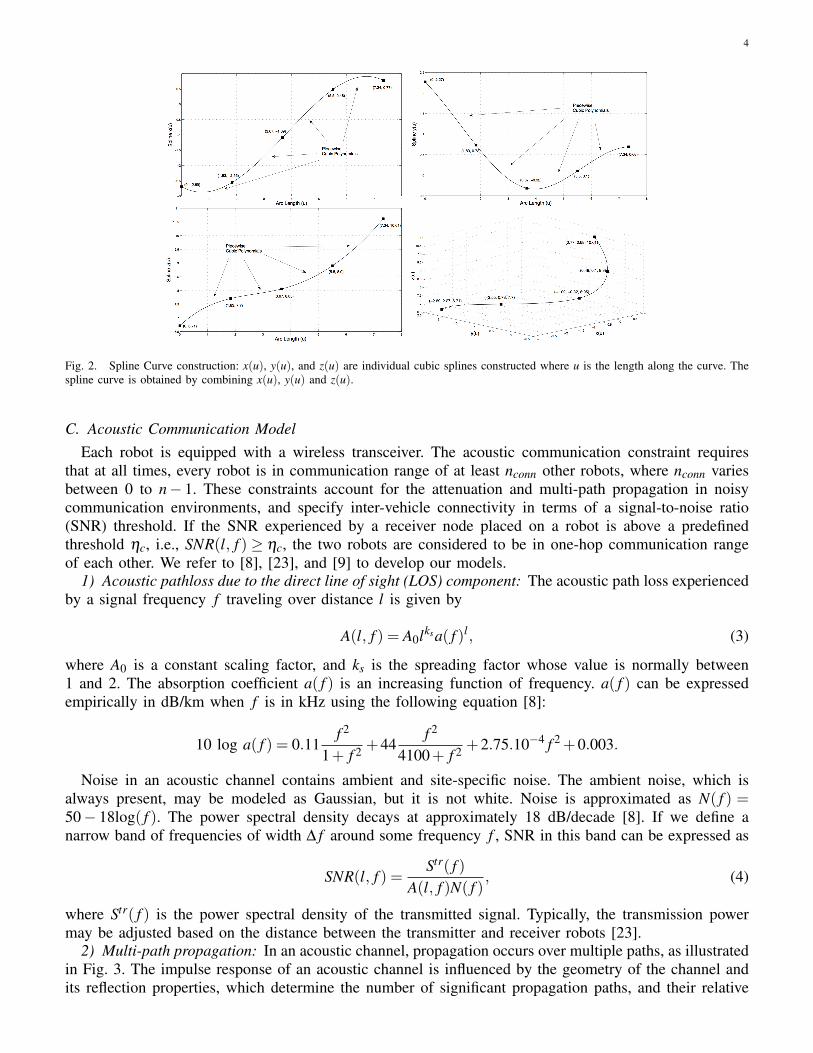
curve is obtained by combining three 1-dimensional piecewise cubic splines, px(u), py(u), and pz(u),where the parameter u is the arc length along the curve. These piecewise cubic splines have continuousfirst derivatives (slope) and second derivatives (curvature) along the curve. The paths represented by the3-dimensional piecewise cubic splines, along with the constraints on the speed, acceleration and turnrate, result in a kinodynamically feasible trajectory. For a detailed discussion on spline curve design andanalysis, readers are referred to [22] and its references. Fig. 2 shows how the spline curve paths areconstructed.

Heave            z  

x  

Y  Sway  

Z  

X  

Y

*  

Yaw  

Pitch  

Roll  

Surge  

Fig. 1. Robot architecture and coordinate system.

4

Fig. 2. Spline Curve construction: x(u), y(u), and z(u) are individual cubic splines constructed where u is the length along the curve. Thespline curve is obtained by combining x(u), y(u) and z(u).

C. Acoustic Communication ModelEach robot is equipped with a wireless transceiver. The acoustic communication constraint requires

that at all times, every robot is in communication range of at least nconn other robots, where nconn variesbetween 0 to n− 1. These constraints account for the attenuation and multi-path propagation in noisycommunication environments, and specify inter-vehicle connectivity in terms of a signal-to-noise ratio(SNR) threshold. If the SNR experienced by a receiver node placed on a robot is above a predefinedthreshold ηc, i.e., SNR(l, f ) ≥ ηc, the two robots are considered to be in one-hop communication rangeof each other. We refer to [8], [23], and [9] to develop our models.

1) Acoustic pathloss due to the direct line of sight (LOS) component: The acoustic path loss experiencedby a signal frequency f traveling over distance l is given by

A(l, f ) = A0lksa( f )l, (3)

where A0 is a constant scaling factor, and ks is the spreading factor whose value is normally between1 and 2. The absorption coefficient a( f ) is an increasing function of frequency. a( f ) can be expressedempirically in dB/km when f is in kHz using the following equation [8]:

10 log a( f ) = 0.11f 2

1+ f 2 +44f 2

4100+ f 2 +2.75.10−4 f 2 +0.003.

Noise in an acoustic channel contains ambient and site-specific noise. The ambient noise, which isalways present, may be modeled as Gaussian, but it is not white. Noise is approximated as N( f ) =50− 18log( f ). The power spectral density decays at approximately 18 dB/decade [8]. If we define anarrow band of frequencies of width ∆ f around some frequency f , SNR in this band can be expressed as

SNR(l, f ) =Str( f )

A(l, f )N( f ), (4)

where Str( f ) is the power spectral density of the transmitted signal. Typically, the transmission powermay be adjusted based on the distance between the transmitter and receiver robots [23].

2) Multi-path propagation: In an acoustic channel, propagation occurs over multiple paths, as illustratedin Fig. 3. The impulse response of an acoustic channel is influenced by the geometry of the channel andits reflection properties, which determine the number of significant propagation paths, and their relative

5

Fig. 3. Geometry of a shallow water channel.

strengths and delays [9]. Since the exact geometry of the channel is unknown, we derive the lower boundson the lengths of the indirect paths.

Bottom reflection: As shown in Fig. 3, (xi,yi,zi) and (x j,y j,z j) are the coordinates of the transmitterand the receiver robots respectively. Consider an arbitrary point (x,y,0) at the bottom of this geometry.The length lbp of a path which is reflected at this arbitrary point is:

lbp =√(x− xi)2 +(y− yi)2 +(zi)2 +

√(x− x j)2 +(y− y j)2 +(z j)2 (5)

Since we do not know all the paths arising due to bottom reflection, we calculate the minimum lengthof these paths. lb denotes the minimum length of a path arising due to bottom reflection. lb is obtainedby evaluating the derivatives

dlbpdx , equation (6), and

dlbpdy , equation (7), and is of the form described in (8).

The path length lbp of any path arising due to bottom reflection will be equal to or greater than lb:

dlbp

dx=

(x− xi)√(x− xi)2 +(y− yi)2 +(zi)2

+(x− x j)√

(x− x j)2 +(y− y j)2 +(z j)2(6)

dlbp

dy=

(y− yi)√(x− xi)2 +(y− yi)2 +(zi)2

+(y− y j)√

(x− x j)2 +(y− y j)2 +(z j)2(7)

lbp ≥ lb =

√(xi− x j)2

4+

(yi− y j)2

4+ z2

i +

√(xi− x j)2

4+

(yi− y j)2

4+ z2

j . (8)

Surface reflection: As shown in Fig. 3, the length lsp of any indirect path which is reflected at anarbitrary point (x,y,h) on the surface is:

lsp =√(x− xi)2 +(y− yi)2 +(h− zi)2 +

√(x− x j)2 +(y− y j)2 +(h− z j)2, (9)

where h is the depth of the acoustic communication area. Similar to (8), the length lsp of any path arisingdue to surface reflection is equal to or greater than the minimum length ls of the surface reflected paths:

lsp ≥ ls =

√(xi− x j)2

4+

(yi− y j)2

4+(h− zi)2 +

√(xi− x j)2

4+

(yi− y j)2

4+(h− z j)2 . (10)

It should be noted that lb and ls can be calculated using the position of the transmitter and receivervehicles.

3) SNR due to multi-path propagation: Since the transmitted signal experiences multi-path propagation,the total power at the receiver is a superposition of the direct (LOS) path and multiple non-LOS paths. Inthe following discussions, the non-LOS paths that have experienced multiple reflections are ignored sincethey experience large attenuation.

Assuming that there are q significant non-LOS paths, the path gain Hp for the p-th non-LOS path isequal to Γp/

√Ap, where p = 1, . . . ,q, Γp is the cumulative reflection coefficient along this path, and Ap

is the propagation loss associated with this path. The p-th non-LOS path acts as a low-pass filter whose

6

transfer function can be modeled as:

Hp(lp, f ) =Γp√

A(lp, f )e− j2π f τp, (11)

where lp is the length of this path, and τp = lp/c is time delay associated with this path. c is the underwaterspeed of sound (1500m/s). e− j2π f τp captures the effect of the phase delay associated with this path.

Incorporating the path gains of the p significant non-LOS paths, the total transfer function and the totalSNR can be described by:

H(l, f ) =1√

A(di j, f )+

q

∑p=1

Γp√A(lp, f )

e− j2π f τp , (12)

SNR(l, f ) =Str( f )N( f )

∥∥∥ 1√A(di j, f )

+q

∑p=1

Γp√A(lp, f )

e− j2π f τp∥∥∥2, (13)

where di j is the Euclidean distance between the transmitter and receiver, and denotes the length of theLOS path.

Since all the non-LOS paths can be divided into two groups, bottom reflected and surface reflectedpaths, the total SNR of the receiver can be expressed as:

SNR(l, f ) =Str( f )N( f )

∥∥∥ 1√A(di j, f )

+q1

∑p=1

Γs√A(lsp, f )

e− j2π f τsp +q2

∑p=1

Γb√A(lbp , f )

e− j2π f τbp

∥∥∥2,

where q1 is the number of non-LOS paths resulting due to surface reflection with reflection coefficientΓs. q2 is the number of non-LOS paths resulting due to bottom reflection with reflection coefficient Γb.It should be noted that q1 +q2 = q.

Utilizing (14) to calculate SNR is non-trivial due to a lack of knowledge of the non-LOS paths. Instead,the worst case SNR, SNRworst , is found using the (known) minimum non-LOS path lengths derived in(8) and (10). SNRworst requires that all non-LOS signals resulting due to multi-path propagation followthe shortest paths with lengths ls or lb, and have a phase delay of π associated with them. SNRworst isexpressed as:

SNRworst(di j, f ) =Str( f )N( f )

‖ 1√A(di j, f )

− q1Γs√A(ls, f )

− q2Γb√A(lb, f )

‖2 (14)

SNRworst provides the lower bound on SNR, and alleviates the need to calculate the actual value of SNR.Instead, providing a lower bound ηc on SNRworst will guarantee the satisfaction of SNR requirements.Also, since SNRworst is a function of di j for a given f , a lower bound on SNRworst implies that thereexists an upper bound (ηd) on the distance between the transmitter and receiver.

SNR(l, f )≥ SNRworst(di j, f ) (15)SNRworst ≥ ηc⇒ SNR(l, f )≥ ηc

SNR(l, f )≥ ηc⇒ di j ≤ ηd

4) One-hop communication connectivity: We introduce a binary variable Ci j(t) that indicates whetherthe two robots are in one-hop communication range of each other or not. Ci j(t)=1 for the robots i andj if they are in one-hop communication range of each other at time t, and Ci j(t)=0 otherwise. Thecommunication constraint requires that each robot be in one-hop communication range of nconn other

7

robots, and can be expressed as:∑

j: j 6=iCi j(t)≥ nconn (16)

Ci j(t) = 1 i f SNRworst ≥ ηc

= 0 i f SNRworst < ηc(17)

Since one-hop communication constraints (16) and (17) are disjunctive in nature (either-or), we refor-mulate them as Big-M constraints given by (18)-(20). For this reformulation, we introduce a constant Mand formulate constraint (19).

In case SNRworst > ηc, Ci j(t) can assume a value of either 0 or 1. The constraint (20) forces at leastnconn of them to be set to 1. This means that only nconn of the Ci j variables, and not necessarily all, areguaranteed to have the correct value Ci j(t) = 1. It is easily seen that if Ci j(t) = 0, then the constraint willbe trivially satisfied for a sufficiently large M.

Ci j(t) ∈ {0,1} (18)

ηc ≤M(1−Ci j(t))+SNRworst (19)

∑j: j 6=i

Ci j(t)≥ nconn, Ci j(t) ∈ {0,1} (20)

D. Receding HorizonThe parameter t represents steps in time. Thor is the receding horizon time. At each time step t, each

robot must calculate its plan for the next Thor time steps, and communicate this plan with other robots inthe network. While the robots compute their trajectory points and corresponding input commands for thenext Thor time steps, only the first of these solutions is implemented, and the process is repeated at eachtime step. Tmax is the time taken by the last-arriving robot to reach its end point. At t = Tmax the scenariois completed. If a robot reaches the goal point before Tmax, it continues to stay there untill the mission isover. However, if required, it can still communicate with other robots.

Each robot plans its own trajectory at each discrete time step by accounting for the plans of all otherrobots. For a given time step t, each robot determines its speed for the next Thor time steps startingtime t, i.e., si(t), . . . ,si(t +Thor), and implements the first speed si(t +1) out of all these speeds. In thisway, the plan starting at time step t + 1 must be computed during time step t. Thus during each timestep t, each robot communicates the following information about its plan P i(t) to other robots: P i(t) =[pi(t) . . .pi(t +Thor)], where pi(t) = (xi(t),yi(t),zi(t)) is the location of the robot i on its path at time t,calculated based on the optimal speed si(t).

E. Decision OrderingThe robots are assigned a pre-determined randomized decision order. The decentralized algorithm

presented here sequentially cycles through each robot, thereby allowing each robot to solve its planningproblem in the order ord(i), i ∈ {1,2, ...,N}.

IV. MODEL FORMULATIONA. Optimization model

Each robot i solves the optimization problem O i(t) indicated by (21)-(33) in the order ord(i) that ithas been assigned.

8

B. Decision VariablesIn (21)-(33), the main decision variables are the speeds, si(t), . . . ,si(t +Thor), for robot i at time t. The

values of the remaining variables are dependent on the speeds.

C. Objective FunctionEquation (21) represents the objective function to be minimized. This formulation forces the robots to

minimize the total distance between their current location and the goal position over the entire recedinghorizon. Constraint (29) defines the distance to goal di

goal(k) for each robot i = 1 . . .n at time-step k,∀k ∈ {t, . . . , t +Thor} as the difference between its path length U i and the total arc length travelled ui(k).The choice of this objective function results in the robots not stalling and moving to their goal positionas fast as possible (minimum time solution).

minimizet+Thor

∑k=t

digoal(k) (21)

subject to ∀ j ∈ {1,2, . . . ,n}, j 6= i

∀k ∈ {t, . . . , t +Thor}(xi(0),yi(0),zi(0)) = oi (22)

ui(0) = 0 (23)

ui(k)≤U i (24)

ui(k) = ui(k−1)+ si(k)∆t (25)

(xi(k),yi(k),zi(k)) = psi(ui(k)) (26)

smin ≤ si(k)≤ smax (27)

amin ≤ ai(k)≤ amax (28)

digoal(k) =U i−ui(k) (29)

di j(k)≥ dsa f e (30)

M(1−Ci j(k))+SNRworst ≥ ηc (31)

∑j: j 6=i

Ci j(k)≥ nconn (32)

Ci j(k) ∈ {0,1} (33)

D. Path (Kinematic) ConstraintsConstraints (22)-(26) define the path of each robot. The constraints (22), (23), and (24) form the

boundary conditions. Constraint (22) indicates that each robot i has to start at a designated start point oi.Constraint (23) initializes the arc length travelled u to zero. Constraint (24) provides the upper bound onthe arc length travelled. Constraint (25) increments the arc length at each time step based on the speed ofthe robot (∆t = 1). Constraint (26) ensures that the robots follow their respective paths as defined by thecubic splines. The function psi(ui(k)) denotes the location of robot i at time step k, ∀k ∈ {t, . . . , t +Thor}after travelling an arc length of ui(k) along the piecewise cubic spline curves. It should be noted thatconstraint (26) is a non-convex nonlinear equality constraint.

E. Speed and Acceleration (Dynamic) ConstraintConstraints (27)-(28) are dynamic constraints that ensure that the speed si(k) (and hence, angular

velocity) and the acceleration ai(k) for each robot i = 1 . . .n at each time step k, ∀k ∈ {t, . . . , t +Thor} are

9

bounded from above (by smax and amax, respectively) and below (by smin and amin, respectively). Theseconstraints are determined by the capabilities of the robot and the curvature of the paths representedby the spline curve. Here we assume that the curvature of the paths is within the achievable bounds ofthe angular speed and radial acceleration of the robots. Hence the angular speed required by the robotscorresponding to the optimal speed is always achievable.

F. Collision Avoidance ConstraintThe non-convex constraint (30) ensures that there is a sufficiently large distance dsa f e between each

pair of robots to avoid a collision at all times.

G. Communication Connectivity ConstraintConstraints (32) and (33) state that vehicle i should be in communication range of at least nconn vehicles.

This means that, for at least nconn values of j = 1, ...,n, j 6= i, the condition SNRworst ≥ ηc should besatisfied. The remaining vehicles may or may not be in communication range of i. In order to expressthis requirement, we introduce a constant M and formulate constraint (31), which states that if Ci j(k)= 1,then vehicles i and j are within communication range. If Ci j(k) = 0, then the constraint will be triviallysatisfied for a sufficiently large M. Constraint (31) is an example of a big-M constraint [24].

H. Decision Making AlgorithmAll robots are initially assumed to be in communication range of each other. The general outline of the

decision-making algorithm is as follows:For any time step t, let each robot i implement the following algorithm:Start: Start at time t.• Step 0 - An order is enforced in terms of which robot plans its trajectory first. The ordering can be

randomly assigned or can be assigned a priori.• Step 1 - Based on its decision order ord(i), each robot i solves the problem O i(t +1) at time t by

taking into account the following plans:1.1 Plans P j(t +1) for robots j, ∀ j ∈ {1,2, . . . ,n}, j 6= i whose ord( j)< ord(i) - these robots have

already calculated their new plans, and1.2 Plans Pζ (t) for robots ζ , ∀ζ ∈ {1,2, . . . ,n}, ζ 6= i whose ord(i) < ord(ζ ) - these robots are

yet to calculate their new plans.• Step 2 -

2.1 If a feasible solution is found, the new plan is P i(t +1).2.2 If O i(t+1) is infeasible, then use the previously available plan P i(t) for the next Thor−1 time

steps, i.e., the new plan

P i(t +1) = P i(t)\pi(t), (34)

where pi(t) = (xi(t),yi(t))• Step 3 - Broadcast this plan to the other robots.End: End by t +1, and repeat.

I. Remarks about the algorithmIn our numerical testing, we found that the decision order ord(i) of the robots i = 1, . . . ,n can qualita-

tively affect the solution of each robot depending on the geometry of the paths.1) Due to the inherent decentralized decision-making, certain robots’ decisions may render the coor-

dination problem difficult to solve for other robots. In some cases, reassigning a different decisionorder ord(i) of the robots i = 1, . . . ,n helped improve overall solutions.

10

TABLE IMOTION AND COMMUNICATION PARAMETER VALUES USED FOR SIMULATIONS

dsa f e 0.02 m smin 0 smax 2.5 m/samin -1 m/s2 amax 0.5 m/s2 M 1000

f 15 KHz h 20 m ks 1.5

2) Also in some cases, certain robots’ decisions can render the coordination problem infeasible forother robots regardless of the decision ordering used. In such cases, the robots may use their plansfrom the previous time steps as indicated by Step 2.2 of the algorithm above.

V. SIMULATIONS AND RESULTSWe focus on studying the effect of acoustic communication constraints on the velocity profiles of the

underwater robots, and on the solution computation times. Additionally, we depict the effect of strictersafety requirements on the velocity profiles of the robots.

A. Simulation SetupThe MATLAB function spline() was used to generate piecewise cubic splines passing through 8

randomly generated waypoints. The spline paths are parametrized by arc length u. The optimization model,defined by (21)-(33) was implemented in MATLAB using the symbolic toolbox and the solver MILANOwas used to perform numerical optimization. The MATLAB-MILANO combination was implemented ona 2.2 GHz Intel Core i7 with 4GB of main memory.

B. SimulationsWe have tested our model for 3 different scenarios that include up to 4 underwater robots and a number

of communications connectivity constraints. In the following discussions, we plot the spline curve paths

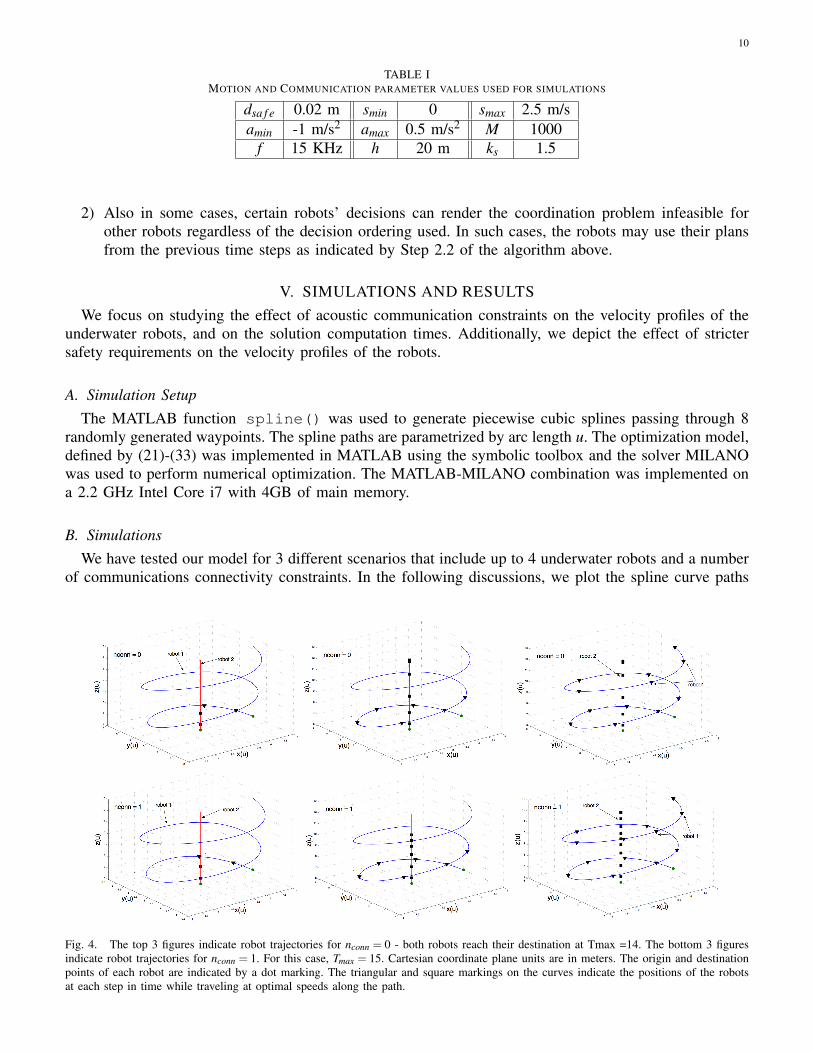
Fig. 4. The top 3 figures indicate robot trajectories for nconn = 0 - both robots reach their destination at Tmax =14. The bottom 3 figuresindicate robot trajectories for nconn = 1. For this case, Tmax = 15. Cartesian coordinate plane units are in meters. The origin and destinationpoints of each robot are indicated by a dot marking. The triangular and square markings on the curves indicate the positions of the robotsat each step in time while traveling at optimal speeds along the path.

11

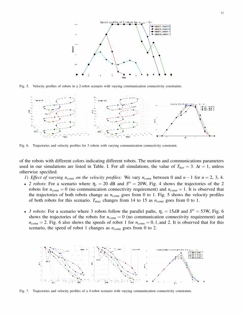
Fig. 5. Velocity profiles of robots in a 2-robot scenario with varying communication connectivity constraints.

Fig. 6. Trajectories and velocity profiles for 3 robots with varying communication connectivity constraint.

of the robots with different colors indicating different robots. The motion and communications parametersused in our simulations are listed in Table. I. For all simulations, the value of Thor = 3. ∆t = 1, unlessotherwise specified.

1) Effect of varying nconn on the velocity profiles: We vary nconn between 0 and n−1 for n = 2, 3, 4.• 2 robots: For a scenario where ηc = 20 dB and Str = 20W, Fig. 4 shows the trajectories of the 2

robots for nconn = 0 (no communication connectivity requirement) and nconn = 1. It is observed thatthe trajectories of both robots change as nconn goes from 0 to 1. Fig. 5 shows the velocity profilesof both robots for this scenario. Tmax changes from 14 to 15 as nconn goes from 0 to 1.

• 3 robots: For a scenario where 3 robots follow the parallel paths, ηc = 15dB and Str = 53W, Fig. 6shows the trajectories of the robots for nconn = 0 (no communication connectivity requirement) andnconn = 2. Fig. 6 also shows the speeds of robot 1 for nconn = 0,1,and 2. It is observed that for thisscenario, the speed of robot 1 changes as nconn goes from 0 to 2.

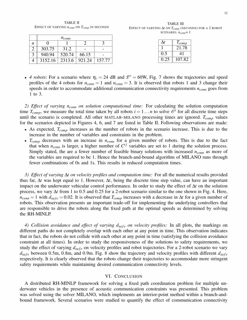
Fig. 7. Trajectories and velocity profiles of a 4-robot scenario with varying communication connectivity constraints.

12

TABLE IIEFFECT OF VARYING nconn ON Tcomp IN SECONDS

nconnn 0 1 2 32 303.75 31.2 - -3 940.94 520.74 66.15 -4 3152.16 2313.6 921.24 157.77

TABLE IIIEFFECT OF VARYING ∆t ON Tcomp (SECONDS) FOR A 2 ROBOT

SCENARIO. nconn= 1

∆t Tcomp1 21.780.5 410.25 107.82

• 4 robots: For a scenario where ηc = 24 dB and Str = 60W, Fig. 7 shows the trajectories and speedprofiles of the 4 robots for nconn = 1 and nconn = 3. It is observed that robots 1 and 3 change theirspeeds in order to accommodate additional communication connectivity requirements nconn goes from1 to 3.

2) Effect of varying nconn on solution computational time: For calculating the solution computationtime Tcomp, we measure the total time taken by all robots i = 1 . . .n to solve O i for all discrete time stepsuntil the scenario is completed. All other MATLAB-MILANO processing times are ignored. Tcomp valuesfor the scenarios depicted in Figures 4, 6, and 7 are listed in Table II. Following observations are made:• As expected, Tcomp increases as the number of robots in the scenario increase. This is due to the

increase in the number of variables and constraints in the problem.• Tcomp decreases with an increase in nconn for a given number of robots. This is due to the fact

that when nconn is larger, a higher number of Ci j variables are set to 1 during the solution process.Simply stated, the are a fewer number of feasible binary solutions with increased nconn as more ofthe variables are required to be 1. Hence the branch-and-bound algorithm of MILANO runs throughfewer combinations of 0s and 1s. This results in reduced computation times.

3) Effect of varying ∆t on velocity profiles and computation time: For all the numerical results providedthus far, ∆t was kept equal to 1. However, ∆t, being the discrete time step value, can have an importantimpact on the underwater vehicular control performance. In order to study the effect of ∆t on the solutionprocess, we vary ∆t from 1 to 0.5 and 0.25 for a 2-robot scenario similar to the one shown in Fig. 4. Here,nconn = 1 with dsa f e = 0.02. It is observed that Tcomp increases with a decrease in ∆t for a given number ofrobots. This observation presents an important trade-off for implementing the underlying controllers thatare responsible to drive the robots along the fixed path at the optimal speeds as determined by solvingthe RH-MINLP.

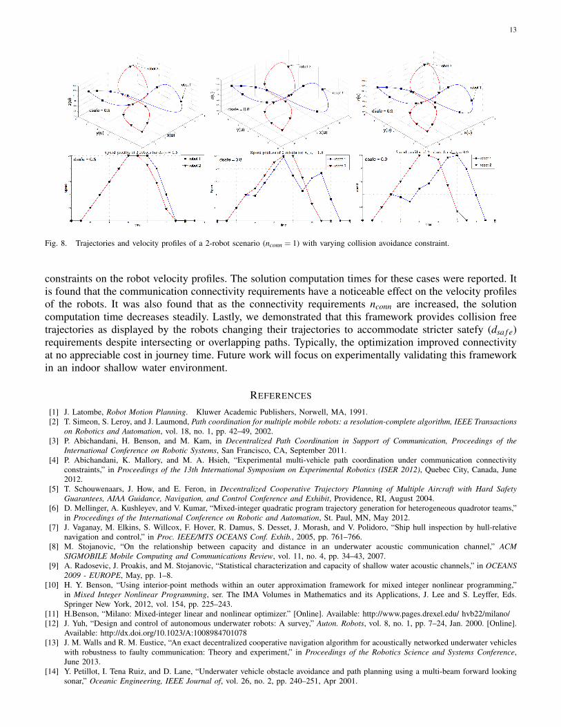
4) Collision avoidance and effect of varying dsa f e on velocity profiles: In all plots, the markings ondifferent paths do not completely overlap with each other at any point in time. This observation indicatesthat in fact, the robots do not collide with each other at any point in time (satisfying the collision avoidanceconstraint at all times). In order to study the responsiveness of the solutions to safety requirements, westudy the effect of varying dsa f e on velocity profiles and robot trajectories. For a 2-robot scenario we varydsa f e between 0.5m, 0.8m, and 0.9m. Fig. 8 show the trajectory and velocity profiles with different dsa f erespectively. It is clearly observed that the robots change their trajectories to accommodate more stringentsafety requirements while maintaining desired communication connectivity levels.

VI. CONCLUSION

A distributed RH-MINLP framework for solving a fixed path coordination problem for multiple un-derwater vehicles in the presence of acoustic communication constraints was presented. This problemwas solved using the solver MILANO, which implements an interior-point method within a branch-and-bound framework. Several scenarios were studied to quantify the effect of communication connectivity

13

Fig. 8. Trajectories and velocity profiles of a 2-robot scenario (nconn = 1) with varying collision avoidance constraint.

constraints on the robot velocity profiles. The solution computation times for these cases were reported. Itis found that the communication connectivity requirements have a noticeable effect on the velocity profilesof the robots. It was also found that as the connectivity requirements nconn are increased, the solutioncomputation time decreases steadily. Lastly, we demonstrated that this framework provides collision freetrajectories as displayed by the robots changing their trajectories to accommodate stricter satefy (dsa f e)requirements despite intersecting or overlapping paths. Typically, the optimization improved connectivityat no appreciable cost in journey time. Future work will focus on experimentally validating this frameworkin an indoor shallow water environment.

REFERENCES

[1] J. Latombe, Robot Motion Planning. Kluwer Academic Publishers, Norwell, MA, 1991.[2] T. Simeon, S. Leroy, and J. Laumond, Path coordination for multiple mobile robots: a resolution-complete algorithm, IEEE Transactions

on Robotics and Automation, vol. 18, no. 1, pp. 42–49, 2002.[3] P. Abichandani, H. Benson, and M. Kam, in Decentralized Path Coordination in Support of Communication, Proceedings of the

International Conference on Robotic Systems, San Francisco, CA, September 2011.[4] P. Abichandani, K. Mallory, and M. A. Hsieh, “Experimental multi-vehicle path coordination under communication connectivity

constraints,” in Proceedings of the 13th International Symposium on Experimental Robotics (ISER 2012), Quebec City, Canada, June2012.

[5] T. Schouwenaars, J. How, and E. Feron, in Decentralized Cooperative Trajectory Planning of Multiple Aircraft with Hard SafetyGuarantees, AIAA Guidance, Navigation, and Control Conference and Exhibit, Providence, RI, August 2004.

[6] D. Mellinger, A. Kushleyev, and V. Kumar, “Mixed-integer quadratic program trajectory generation for heterogeneous quadrotor teams,”in Proceedings of the International Conference on Robotic and Automation, St. Paul, MN, May 2012.

[7] J. Vaganay, M. Elkins, S. Willcox, F. Hover, R. Damus, S. Desset, J. Morash, and V. Polidoro, “Ship hull inspection by hull-relativenavigation and control,” in Proc. IEEE/MTS OCEANS Conf. Exhib., 2005, pp. 761–766.

[8] M. Stojanovic, “On the relationship between capacity and distance in an underwater acoustic communication channel,” ACMSIGMOBILE Mobile Computing and Communications Review, vol. 11, no. 4, pp. 34–43, 2007.

[9] A. Radosevic, J. Proakis, and M. Stojanovic, “Statistical characterization and capacity of shallow water acoustic channels,” in OCEANS2009 - EUROPE, May, pp. 1–8.

[10] H. Y. Benson, “Using interior-point methods within an outer approximation framework for mixed integer nonlinear programming,”in Mixed Integer Nonlinear Programming, ser. The IMA Volumes in Mathematics and its Applications, J. Lee and S. Leyffer, Eds.Springer New York, 2012, vol. 154, pp. 225–243.

[11] H.Benson, “Milano: Mixed-integer linear and nonlinear optimizer.” [Online]. Available: http://www.pages.drexel.edu/ hvb22/milano/[12] J. Yuh, “Design and control of autonomous underwater robots: A survey,” Auton. Robots, vol. 8, no. 1, pp. 7–24, Jan. 2000. [Online].

Available: http://dx.doi.org/10.1023/A:1008984701078[13] J. M. Walls and R. M. Eustice, “An exact decentralized cooperative navigation algorithm for acoustically networked underwater vehicles

with robustness to faulty communication: Theory and experiment,” in Proceedings of the Robotics Science and Systems Conference,June 2013.

[14] Y. Petillot, I. Tena Ruiz, and D. Lane, “Underwater vehicle obstacle avoidance and path planning using a multi-beam forward lookingsonar,” Oceanic Engineering, IEEE Journal of, vol. 26, no. 2, pp. 240–251, Apr 2001.

14

[15] C. Petres, Y. Pailhas, P. Patron, Y. Petillot, J. Evans, and D. Lane, “Path planning for autonomous underwater vehicles,” IEEETransactions on Robotics, vol. 23, no. 2, pp. 331–341, April 2007.

[16] R. Smith, A. Pereira, Y. Chao, P. Li, D. Caron, B. Jones, and G. Sukhatme, “Autonomous underwater vehicle trajectory design coupledwith predictive ocean models: A case study,” in Robotics and Automation (ICRA), 2010 IEEE International Conference on, May, pp.4770–4777.

[17] P. Encarnacao and A. Pascoal, “3d path following for autonomous underwater vehicle,” in Proceedings of the 39th IEEE Conferenceon Decision and Control, vol. 3, 2000, pp. 2977–2982 vol.3.

[18] R. Ghabcheloo, A. Aguiar, A. Pascoal, and C. Silvestre, “Coordinated path-following control of multiple auvs in the presenceof communication failures and time delays,” in Proceedings of the 7th Conference on Maneuvering and Control of Marine Craft(MCMC2006), Sept 2006.

[19] N. Yilmaz, C. Evangelinos, P. F. J. Lermusiaux, and N. Patrikalakis, “Path planning of autonomous underwater vehicles for adaptivesampling using mixed integer linear programming,” IEEE Journal of Oceanic Engineering,, vol. 33, no. 4, pp. 522–537, Oct. 08.

[20] S. E. Webster, R. M. Eustice, H. Singh, and L. Whitcomb., “Advances in single-beacon one-way-travel-time acoustic navigation forunderwater vehicles,” The International Journal of Robotics Research, vol. 31, no. 8, pp. 935–950, July 2012.

[21] T. Fossen, Guidance and control of ocean vehicles. Wiley, 1994. [Online]. Available:http://books.google.com/books?id=cwJUAAAAMAAJ

[22] M.Lepetic, G. Klancar, I. Skrjanc, D. Matko, and B. Potocnik, “Time optimal path planning considering acceleration limits,” Roboticsand Autonomous Systems, vol. 45, pp. 199–210, 2003.

[23] M. Stojanovic, “Underwater acoustic communications: Design considerations on the physical layer,” in Fifth Annual Conference onWireless on Demand Network Systems and Services (WONS 2008), Jan. 2008, pp. 1–10.

[24] A. Bemporad and M. Morari, Control of Systems Integrating Logic, Dynamics, and Constraints, Automatica, vol. 35, pp. 407–427,1999.

Solmaz Torabi received her B.S. degree in Electrical Engineering from Sharif University of Technology, Tehran, Iran,in 2011. Her research interests are in the areas of acoustic communication and optimal decision-making. She currentlyworks as a research assistant at Drexel University’s Electrical and Computer Engineering department.

Shambadeb Basu received his B.Tech. degree from West Bengal University of Technology, Calcutta, India. Subsequentto this, he worked as a Research Fellow at Jadavpur University, Calcutta, India. His interests are in control and motionplanning for autonomous underwater robots. He currently works as a research assistant at Drexel University’s Electricaland Computer Engineering department.

Hande Benson is an Associate Professor at the Decision Sciences Department in the LeBow College of Business ofDrexel University. Her research interests lie in the field of nonlinear programming, particularly in using interior-pointmethods to solve large-scale optimization problems. Research sponsors include the National Science Foundation (NSF)and the Office of Naval Research (ONR).

Pramod Abichandani is a Senior Researcher and an Assistant Teaching Professor at Drexel University. His researchinterests are centered around optimal, multi-dimensional, data-driven decision-making, through the use of techniquesfrom mathematical programming, linear and nonlinear systems theory, statistics, and machine learning. Researchsponsors include the Office of Naval Research (ONR), Mathworks, and Drexel University.