1 A Max-Flow Based Approach to the Identiï¬cation of Protein

1

A Max-Flow Based Approach to the

Identification of Protein Complexes Using

Protein Interaction and Microarray Data†

Jianxing Feng, Rui Jiang∗, and Tao Jiang∗

Abstract

The emergence of high-throughput technologies leads to abundant protein-protein interaction (PPI)

data and microarray gene expression profiles, and provides agreat opportunity for the identification

of novel protein complexes using computational methods. Bycombining these two types of data, we

propose a novelGraph Fragmentation Algorithm(GFA) for protein complex identification. Adapted

from a classical max-flow algorithm for finding the (weighted) densest subgraphs, GFA first finds large

(weighted) dense subgraphs in a protein-protein interaction network and then breaks each such subgraph

into fragments iteratively by weighting its nodes appropriately in terms of their corresponding log fold

changes in the microarray data, until the fragment subgraphs are sufficiently small. Our tests on three

widely used protein-protein interaction datasets and comparisons with several latest methods for protein

complex identification demonstrate the strong performanceof our method in predicting novel protein

complexes in terms of its specificity and efficiency. Given the high specificity (or precision) that our

method has achieved, we conjecture that our prediction results imply more than 200 novel protein

complexes.

Index Terms

Protein complex, protein-protein interaction network, microarray, dense subgraph, maximum net-

work flow, efficient algorithm

Jianxing Feng is with Department of Computer Science and Technology, Tsinghua University, Beijing 100084, China. Email:

[email protected]

Rui Jiang is with MOE Key Laboratory of Bioinformatics, Bioinformatics Division TNLIST/Department of Automation,

Tsinghua University, Beijing 100084, China. Email: [email protected]

Tao Jiang is with Department of Computer Science, University of California, Riverside, CA 92521. Email: [email protected]

∗ To whom correspondence should be addressed.

† An extended abstract of this paper has been presented at the7th Annual International Conference on Computational Systems

Bioinformatics (CSB), August, 2008, Stanford, CA.

December 31, 2009 DRAFT

2

I. I NTRODUCTION

With the advances in modern biophysics and biochemistry, ithas been widely accepted that the

rise of complicated biological functions is largely due to the cooperative effects of multiple genes

and/or gene products. This understanding leads to the emergence of high-throughput technologies

for identifying interactions between biological molecules and results in the prosperity of interac-

tomics in the post genomics and proteomics era. For example,with the use of yeast two-hybrid

assays [1], [2], [3] and pull-down mass spectrometry experiments [4], [5], genome-wide protein-

protein interactions (PPIs) have been identified and encoded into global PPI networks for the

model speciesSaccharomyces cerevisiae(i.e., baker’s yeast) [6], [7], [8]. With the improvement

of instruments and increase in the throughput, these technologies have also been applied to

identify interactions of human proteins, providing an increasing understanding of the global

human PPI network [9]. Parallel to the boom of high-throughput identification of PPIs, genome-

wide microarray experiments regarding the expression of genes across a number of different

conditions have also been conducted and resulted in publicly available databases such as the

gene expression omnibus[10].

As a major form of the collaborative effects of two or more proteins, protein complexes play

important roles in the formation of complicated biologicalfunctions such as the transcription of

DNA, the translation of mRNA,etc. Traditionally, protein complexes are identified using exper-

imental techniques such as co-immunoprecipitation and mass spectrometry-based approaches,

or computational methods such as protein-protein docking based on protein structures. These

methods, though successful, can hardly meet the requirement of identifying all protein complexes

in known organisms, due to the large number of proteins that exist and the cost of biological

experiments. On the other hand, since in most known cases, a protein complex is composed

of a group of two or more proteins that are associated by stable protein-protein interactions,

computational methods that can make use of abundant data given by the above high-throughput

technologies have been demonstrating increasing success [11], [12], [13], [14], [15].

Many studies use PPI data alone for the purpose of identifying protein complexes or bio-

logically functional modules. These methods assume that densely connected components in PPI

networks are likely to form functional modules and hence arelikely to be protein complexes

[16]. Under this assumption, the methods generally use the density of interactions as a main


3

criterion and identify protein complexes by finding dense regions in PPI networks. To mention a

few, Bader and Hogue [11] proposed a clustering algorithm called MCODE that isolates dense

regions in a PPI network by weighting each vertex according to the topological properties of

its neighborhood. Andreopouloset al. [17] presented a layered clustering algorithm that groups

proteins by the similarity of their direct neighborhoods. Spirin and Mirny [12] applied three

methods (i.e., clique enumeration, super paramagnetic clustering, and Monte Carlo simulation)

to an older version of the MIPS PPI network for yeast [7] and produced about 100 dense

subgraphs that were predicted to be protein complexes. Their result was found to be superior

to many others in terms of the specificity. Pei and Zhang [13] introduced a subgraph quality

measure as well as a “seed-refine” algorithm to search for possible protein complexes in a PPI

network. Kinget al. [18] gave a clustering algorithm based on restricted neighborhood search

to partition a PPI network into clusters using some cost function. Bu et al. [19] introduced a

spectral method derived from graph theory to uncover hiddentopological structures that consist

of biologically relevant functional groups. Wanget al. [20] incorporated both a global metric

and a local metric to dissect PPI networks. Liet al. [14] found maximal dense regions by

merging local cliques according to their affinity. In a subsequent work, Li et al. [15] devised

an algorithm, called DECAFF, to address two major issues in current high-throughout PPI data,

namely, incompleteness and high data noise.

Another group of methods combine PPI data and microarray gene expression profiles for

the purpose of identifying protein complexes or functionalmodules. For example, Segalet al.

combined PPI and microarray data to identify pathways [21].Chen and Yuan [22] extended

a betweenness-based partition algorithm to partition PPI networks with weighted edges using

microarray data. Idekeret al. used such a combination to search for regulatory modules and

signalling circuits [23]. Guoet al. [24] identified condition-responsive sub-networks in a PPI

network by weighting its edges based on gene expression profiles. The program MATISSE

presented in [25] combines PPI and microarray data to find tissue/condition specific functional

modules. The work was recently followed up in [26] with the introduction of another program,

called CEZANNE, that takes advantage of weighted PPI networks whose interactions have been

assigned reliable confidence scores.

These methods regard PPIs as static descriptions of the potentially collaborative effects be-

tween proteins and treat gene expression profiles as dynamicinformation of genes under various


4

conditions. Since proteins of a complex usually work together to complete certain biological

functions, and there exists a simple mapping between genes and the proteins, the combination

of PPI and microarray data could clearly help the discovery of protein complexes or functional

modules. For the identification of protein complexes, an important question is that to what

extent known complexes exhibit co-expression of their members. Jansenet al. investigated this

problem on yeast [27]. They found that generally, permanentcomplexes, such as the ribosome

and proteasome, have a particularly strong relationship with expression, while transient ones do

not. This result has been confirmed by similar work such as [28] and [29]. In [28], Simoniset al.

found that “stable“ complexes such as cytoplasmic ribosomeand the proteasome are coherently

up or down-regulated in many different conditions. However, such coherency is detected at some

level in only 71 out of 113 complexes containing at least 5 proteins. These work generally showed

that the members of some complexes are correlated in their expressions while the members of

the other complexes are not. Therefore, methods for identifying protein complexes that are solely

based on expression profiles may not be very reliable.

Besides these methods, there exist some other methods that aim at identifying protein com-

plexes by using comparative interactomics. For example, Sharan et al. [30] identified protein

complexes by a comparative analysis of the PPI networks fromyeast and bacteria. Hirsh and

Sharan [31] developed a probabilistic model for protein complexes that are conserved across two

species and applied it to yeast and fly. These methods based oncomparative analysis require

the availability of quality PPI networks from multiple species and can only identify protein

complexes conserved in multiple species. See [32], [33], [34] for more information about aligning

and comparing multiple PPI networks.

Despite differences in the approach and the use of data, mostof the computational methods

mentioned above define the density of a subgraph as the numberof its edges over the number

of all possible edges in the subgraph and follow a bottom-up local search strategy to find

dense subgraphs. For example, Liet al. [15] first found small dense subgraphs (or components)

in a PPI network and then merged these components gradually to form protein complex-like

subgraphs. Pei and Zhang [13] greedily expanded some carefully selected seed subgraphs until

a given criterion was met. Because such a local search strategy in general does not return an

optimal solution (with respect to most objective functions), the above bottom-up methods are

not guaranteed to find the densest subgraphs in the input PPI network and therefore may miss


5

some important protein complexes that are actually dense.

To overcome this drawback, we adopt a new definition of the density of a subgraph (i.e., the

number of edges over the number of nodes in the subgraph) and present a top-down method that

utilizes the density information in PPI networks explicitly as well as microarray gene expression

profiles to identify protein complexes. Our work combines the classic maximum network flow

basedDensest Subgraph Algorithm(DSA) [35] to find the densest subgraphs with a novel

application of microarray data. Our algorithm, named theGraph Fragmentation Algorithm(GFA),

first finds dense subgraphs in a PPI network, many of which could potentially be large, and

breaks each of them into fragments iteratively by weightingits nodes appropriately in terms of

their corresponding log fold changes in the microarray data, until the fragment subgraphs are

sufficiently small. An important property of GFA is that it mainly utilizes the protein interaction

information so that its performance will not be seriously affected by the possible inconsistency

among the expression profiles of the members of a complex.

In order to test the performance of our method, we apply GFA tothree widely used yeast PPI

networks (i.e., the MIPS, DIP and BioGRID PPI networks) and compare our predictions with

the known protein complexes in the MIPS database as well as with those of the latest methods

for protein complex identification (that are not based on comparative analysis) given in [23],

[11], [36], [25], [37], [15], [26]. The test results clearlydemonstrate the superior performance

of our method in predicting novel protein complexes in termsof specificity and efficiency (to

be defined below). For example, GFA could be tuned to achieve ahigh specificity of 81%

while maintaining its sensitivity at 71% on the DIP PPI network. Our method also provides a

ranking of the predicted complexes, taking advantage of themultiple conditions (or samples) in

the microarray expression data. Predicted complexes with higher ranks are supported by more

samples and thus have larger likelihoods to be true protein complexes. Moreover, our predictions

result in more than 200 highly ranked dense subgraphs that share little common proteins with

the known complexes in MIPS and are thus likely to be novel protein complexes.

II. M ATERIALS AND METHODS

A. Data sources

Three PPI datasets concerningSaccharomyces cerevisiae(i.e., baker’s yeast) are used. The

first one is the MIPS protein-protein interaction network [7], which contains manually compiled


6

interactions from the literature and published large-scale experiments. This dataset will simply

be denoted as MIPS-PPI. The second one is the DIP protein-protein interaction network [6],

denoted as DIP-PPI. The third one is BioGRID protein-protein interaction network [8], which

is the most comprehensive one and will be denoted as BioGRID-PPI. The file names, which

contains the download dates or release numbers, of the threedatasets are PPI18052006.tab,

Scere20081014.txt and BIOGRIDPPI 2.0.35 for MIPS, DIP and BioGRID-PPI, respectively.

Because a PPI network is treated as an undirected simple graph, at most one edge will be kept

between any pair of proteins. The numbers of nodes (or edges)in the MIPS, DIP and BioGRID

PPI networks are 4,554 (or 12,319), 4,947 (or 17,257) and 5,201 (or 71,044), respectively.

We retrieved 51 sets of microarray gene expression data concerning yeast from the GEO

database [10] where the log fold changes of expression levels are provided. Each dataset contains

multiple samples (or conditions). Totally, 824 samples arecontained in the 51 datasets. Since

the genes expressed in each sample are different and they could also be different from the genes

contained in a PPI network, we will use a sample of the microarray data on a PPI network

if it covers at least 90% of the genes in the network under consideration. For genes that have

no expression data in a certain sample, we treat their (log transformed) expression values as 0.

Finally, we chose (randomly) 500, 600, and 700 samples to be applied on the MIPS, DIP, and

BioGRID PPI networks, respectively.

As in previous studies [11], [12], [14], [15], the MIPS complex database [7] is used as the

benchmark (i.e., the truth) to evaluate the protein complexes predicted by our method.1 This

database contains protein complexes verified manually and those identified by high throughput

experiments. We use the manually verified complexes as the benchmark, denoted as MIPS-

MAN. Furthermore, our algorithm GFA only outputs connectedsubgraphs, but many complexes

in MIPS-MAN are not connected in the above PPI networks. To evaluate our results more

reasonably, we decompose each MIPS complex into connected components according to the PPI

network under study. We will use MIPS-MAN-COMP to denote the sets of connected complex

components obtained from MIPS-MAN. Finally, since GFA mainly focuses on complexes form-

ing dense subgraphs in the PPI networks, it does not output subgraphs consisting of a single node

1Note that since MIPS complexes are not extracted (computationally) fromMIPS-PPI and vise versa, they could serve as a

valid benchmark for predicting complexes from MIPS-PPI.


7

or edge (because they are trivial). Therefore, all complexes or complex components with sizes

1 or 2 are removed from MIPS-MAN-COMP. Note that the actual content of the benchmark

MIPS-MAN-COMP depends on the underlying PPI network used. The size of MIPS-MAN-

COMP is defined as the number of complexes or complex components in the benchmark. On

the MIPS, DIP and BioGRID PPI networks, the sizes of MIPS-MAN-COMP are 100, 114 and

134, respectively.2 The numbers of complexes and complex components with sizes above 20,

30 and 40 are 0, 1 and 2 in the three MIPS-MAN-COMP benchmarks corresponding to the

MIPS, DIP and BioGRID PPI networks, respectively. Besides MIPS-MAN and MIPS-MAN-

COMP, we will also use the biological process and macromolecular complex categories in Gene

Ontology (GO) [38] as benchmarks for additional comparisons with the programs CODEC [37]

and CEZANNE [26]. MIPS-MAN and these last two benchmarks fromGO were used in [26]

to compare methods for finding functional modules in PPI networks.

B. An outline of GFA

A PPI network is considered as an undirected simple graph, where each node represents a

protein, and each edge represents an interaction between two nodes. A common strategy for

discovering protein complexes from a given PPI network is tosearch for dense subgraphs in

the network. Many methods based on such a strategy have been proposed in the literature as

reviewed in Section I. The density of a subgraph could be defined in several ways. A widely

used definition of density isδ = 2 · |E|/(|V | · (|V | − 1)) [11], [12], whereE andV denote the

sets of edges and nodes in the subgraph, respectively. A niceproperty of this definition is that

δ is in [0, 1]. Another possible definition isδ = |E|/|V |. Both definitions are sensitive to the

size (i.e., the number of nodes) of a subgraph. It is easy to see that the first definition favors

small subgraphs, as demonstrated in [12], while the second one favors large subgraphs. In fact,

when the first definition is applied, we have to add a lower bound on |V | to make the result

interesting. We will use the latter definition of density in this work, since there is an elegant

algorithm to find the densest subgraph under this definition.Our experimental results will also

demonstrate that this definition of density works very well in finding protein complexes.

Theoretically, the problem of finding a subgraph with the greatest density in a graph under

2These three datasets are provided as online supplementary material.


8

the first definition is much harder than that under the second one. The problem under the first

definition is basically equivalent to finding the largest clique in a graph, a classical NP-hard

problem in theoretical computer science [39]. However, there is an elegant and fast algorithm to

solve the problem under the second density definition. This algorithm, simply denoted as DSA

(i.e., theDensest Subgraph Algorithm), finds a densest subgraph in a graph by iteratively solving

a series of maximum flow problems and has the time complexity of O(|E| · |V | · log(|V |2/|E|))

[35]. Although DSA can be iterated to find many dense subgraphs in a PPI network, this approach

(alone) will likely not work very well in terms of finding protein complex-like subgraphs, since it

tends to find large dense subgraphs while protein complexes are usually small (i.e., containing no

more than 20 proteins). Nevertheless, DSA will form the coreingredient of our algorithm GFA

for finding protein complexes. GFA actually uses a generalized version of the second density

definition:δ = |E|/w(V ), where we assume that the nodes in the graph are weighted (e.g., using

the log fold changes in some sample of microarray data) andw(V ) denotes the total weight of

the nodes in the subgraph. The algorithm DSA mentioned abovealso works for this generalized

definition.

GFA consists of two phases: (1) identify candidate subgraphs from the input PPI network using

a single sample of gene expression data, and (2) combine candidate subgraphs from multiple

samples to form a ranked list of predicted protein complexes. The basic idea behind the first

phase is to iterate DSA to obtain (large) dense subgraphs andthen break each large dense

subgraph into fragment subgraphs by weighting its nodes appropriately using the log fold changes

of the nodes in the sample. This phase is executed on each sample separately. In the second

phase, we have to detect and remove redundant (or overlapping) subgraphs found using different

samples and rank the subgraphs according to the times that they are found in all samples. The

worst case time complexity of GFA, largely determined by thetime complexity of phase 1, is

O(|E| · |V |2 · log(|V |2/|E|) · MaxIter · SampleSize), 3 where the parameterMaxIter limits the

number of times that DSA will be iterated to output a single dense subgraph, andSampleSize

is the number of samples of the microarray data used in the computation.

3Note that when each sample is used, at most|V | dense subgraphs could be extracted by GFA. Thus, GFA may iterate DSA

|V | times on a sample. Clearly, this is a highly conservative estimation of the time complexity of GFA.


9

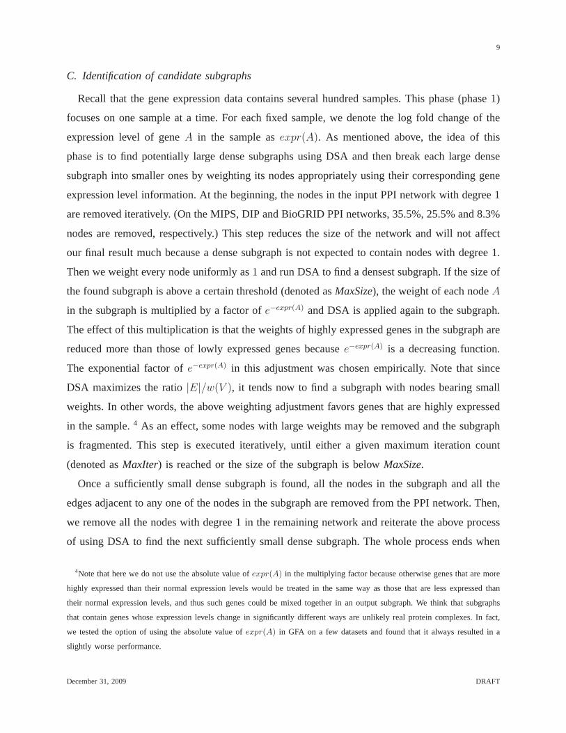
C. Identification of candidate subgraphs

Recall that the gene expression data contains several hundred samples. This phase (phase 1)

focuses on one sample at a time. For each fixed sample, we denote the log fold change of the

expression level of geneA in the sample asexpr(A). As mentioned above, the idea of this

phase is to find potentially large dense subgraphs using DSA and then break each large dense

subgraph into smaller ones by weighting its nodes appropriately using their corresponding gene

expression level information. At the beginning, the nodes in the input PPI network with degree 1

are removed iteratively. (On the MIPS, DIP and BioGRID PPI networks, 35.5%, 25.5% and 8.3%

nodes are removed, respectively.) This step reduces the size of the network and will not affect

our final result much because a dense subgraph is not expectedto contain nodes with degree 1.

Then we weight every node uniformly as1 and run DSA to find a densest subgraph. If the size of

the found subgraph is above a certain threshold (denoted asMaxSize), the weight of each nodeA

in the subgraph is multiplied by a factor ofe−expr(A) and DSA is applied again to the subgraph.

The effect of this multiplication is that the weights of highly expressed genes in the subgraph are

reduced more than those of lowly expressed genes becausee−expr(A) is a decreasing function.

The exponential factor ofe−expr(A) in this adjustment was chosen empirically. Note that since

DSA maximizes the ratio|E|/w(V ), it tends now to find a subgraph with nodes bearing small

weights. In other words, the above weighting adjustment favors genes that are highly expressed

in the sample.4 As an effect, some nodes with large weights may be removed andthe subgraph

is fragmented. This step is executed iteratively, until either a given maximum iteration count

(denoted asMaxIter) is reached or the size of the subgraph is belowMaxSize.

Once a sufficiently small dense subgraph is found, all the nodes in the subgraph and all the

edges adjacent to any one of the nodes in the subgraph are removed from the PPI network. Then,

we remove all the nodes with degree 1 in the remaining networkand reiterate the above process

of using DSA to find the next sufficiently small dense subgraph. The whole process ends when

4Note that here we do not use the absolute value ofexpr(A) in the multiplying factor because otherwise genes that are more

highly expressed than their normal expression levels would be treated in the same way as those that are less expressed than

their normal expression levels, and thus such genes could be mixed together in an output subgraph. We think that subgraphs

that contain genes whose expression levels change in significantly different ways are unlikely real protein complexes. In fact,

we tested the option of using the absolute value ofexpr(A) in GFA on a few datasets and found that it always resulted in a

slightly worse performance.


10

the PPI network exhausts. Note that although this step of GFAfavors highly expressed genes

when it has to break a large dense subgraph returned by DSA into smaller subgraphs, it may

very well identify many candidate dense subgraphs consisting of genes with arbitrary expression

levels that are not very large (and thus do not have to be broken up).

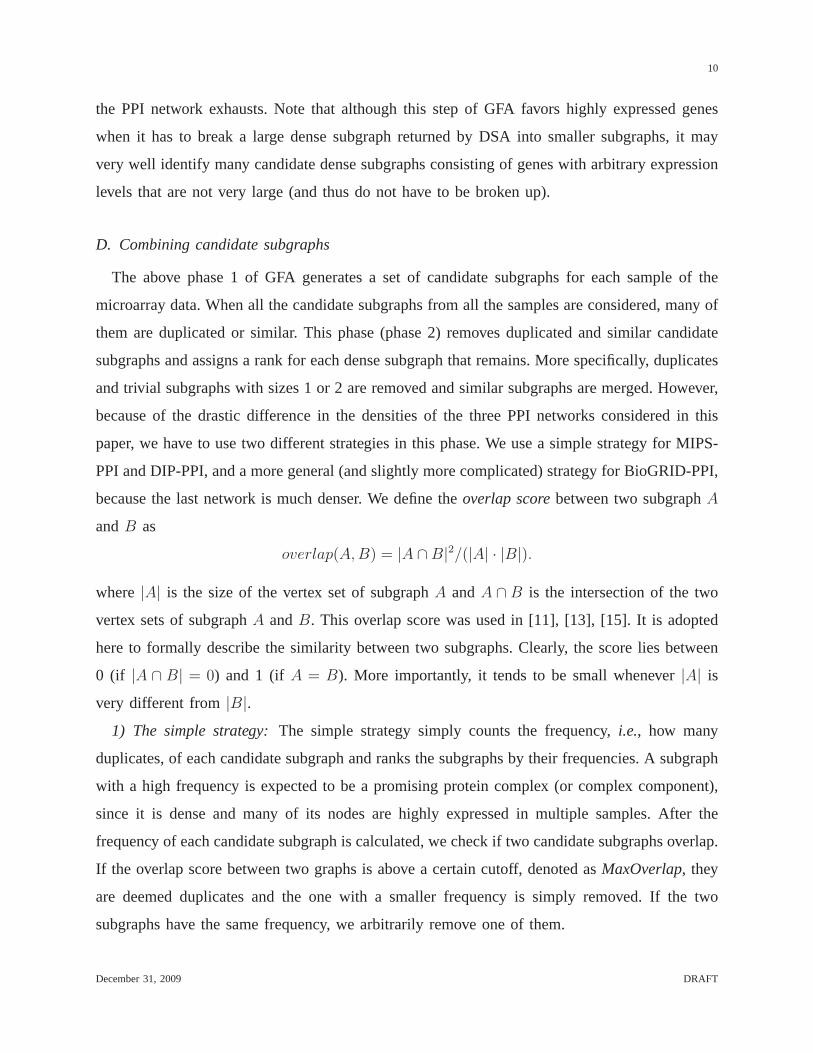
D. Combining candidate subgraphs

The above phase 1 of GFA generates a set of candidate subgraphs for each sample of the

microarray data. When all the candidate subgraphs from all the samples are considered, many of

them are duplicated or similar. This phase (phase 2) removesduplicated and similar candidate

subgraphs and assigns a rank for each dense subgraph that remains. More specifically, duplicates

and trivial subgraphs with sizes 1 or 2 are removed and similar subgraphs are merged. However,

because of the drastic difference in the densities of the three PPI networks considered in this

paper, we have to use two different strategies in this phase.We use a simple strategy for MIPS-

PPI and DIP-PPI, and a more general (and slightly more complicated) strategy for BioGRID-PPI,

because the last network is much denser. We define theoverlap scorebetween two subgraphA

andB as

overlap(A,B) = |A ∩B|2/(|A| · |B|).

where|A| is the size of the vertex set of subgraphA andA ∩ B is the intersection of the two

vertex sets of subgraphA andB. This overlap score was used in [11], [13], [15]. It is adopted

here to formally describe the similarity between two subgraphs. Clearly, the score lies between

0 (if |A ∩ B| = 0) and 1 (if A = B). More importantly, it tends to be small whenever|A| is

very different from|B|.

1) The simple strategy:The simple strategy simply counts the frequency,i.e., how many

duplicates, of each candidate subgraph and ranks the subgraphs by their frequencies. A subgraph

with a high frequency is expected to be a promising protein complex (or complex component),

since it is dense and many of its nodes are highly expressed inmultiple samples. After the

frequency of each candidate subgraph is calculated, we check if two candidate subgraphs overlap.

If the overlap score between two graphs is above a certain cutoff, denoted asMaxOverlap, they

are deemed duplicates and the one with a smaller frequency issimply removed. If the two

subgraphs have the same frequency, we arbitrarily remove one of them.


11

As shown in our experimental results, this simple strategy works very well on MIPS-PPI and

DIP-PPI, mainly due to the sparsity of these networks. For BioGRID-PPI which is much denser,

however, the simple strategy does not perform as well as for sparse networks. This is mainly

due to the fact that a dense network such as BioGRID-PPI usuallycontains a large number of

dense subgraphs and the sizes of dense subgraphs tend to be large too. Consequently, a large

number of microarray samples are needed in order to make the frequencies of dense subgraphs

sufficiently high. Therefore, when a limited number of microarray samples are available, the

simple strategy could become too conservative since it onlycounts subgraphs that repeat exactly

in all the candidate subgraphs.

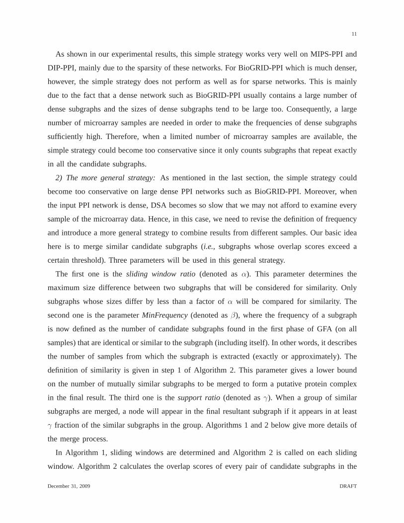
2) The more general strategy:As mentioned in the last section, the simple strategy could

become too conservative on large dense PPI networks such as BioGRID-PPI. Moreover, when

the input PPI network is dense, DSA becomes so slow that we maynot afford to examine every

sample of the microarray data. Hence, in this case, we need torevise the definition of frequency

and introduce a more general strategy to combine results from different samples. Our basic idea

here is to merge similar candidate subgraphs (i.e., subgraphs whose overlap scores exceed a

certain threshold). Three parameters will be used in this general strategy.

The first one is thesliding window ratio (denoted asα). This parameter determines the

maximum size difference between two subgraphs that will be considered for similarity. Only

subgraphs whose sizes differ by less than a factor ofα will be compared for similarity. The

second one is the parameterMinFrequency(denoted asβ), where the frequency of a subgraph

is now defined as the number of candidate subgraphs found in the first phase of GFA (on all

samples) that are identical or similar to the subgraph (including itself). In other words, it describes

the number of samples from which the subgraph is extracted (exactly or approximately). The

definition of similarity is given in step 1 of Algorithm 2. This parameter gives a lower bound

on the number of mutually similar subgraphs to be merged to form a putative protein complex

in the final result. The third one is thesupport ratio (denoted asγ). When a group of similar

subgraphs are merged, a node will appear in the final resultant subgraph if it appears in at least

γ fraction of the similar subgraphs in the group. Algorithms 1and 2 below give more details of

the merge process.

In Algorithm 1, sliding windows are determined and Algorithm 2 is called on each sliding

window. Algorithm 2 calculates the overlap scores of every pair of candidate subgraphs in the


12

Algorithm 1 MergeSubgraphsMain1: Let U be the max size of all the candidate subgraphs.

2: for i = U + 1 down to 4do

3: u← i.

4: l← u− 1− ⌊α · u⌋.

5: MergeSubgraphs(u, l).

6: end for

7: Delete each merged subgraph that overlaps with another merged subgraph by a score greater

than the given cutoffMaxOverlap.

Algorithm 2 MergeSubgraphs(u, l)1: Create a similarity graphG. Each node inG corresponds to a subgraph with size in range

[l, u). There is an edge between nodesA andB if and only if the two subgraphsGA and

GB represented byA andB are similar,i.e., overlap(GA, GB) ≥ q · q/(l · (u− 1)), where

q = l − ⌊α · l⌋.

2: DecomposeG into disjoint cliques by repeatedly finding and removing maximal cliques in

G.

3: For each cliqueC, suppose that the set of subgraphs corresponding toC is {S1, S2, . . . , Sm}.

If m ≥ β, create a new subgraphS as follows: an element (protein) is contained inS if

and only if it appears in at leastγ ·m of the m subgraphsS1, S2, . . . , Sm.

4: Remove all the candidate subgraphs that have been merged.

sliding window and merges each group (i.e., clique) of subgraphs that are mutually similar if the

group is large enough. Each candidate subgraph being mergedis removed so that every subgraph

is merged once in the whole process.

The sliding window sizeu − l = ⌊α · u⌋ increases with the size of candidate subgraphs that

are processed. We may interpret the parameterq in Algorithm 2 as the minimum number of

nodes and edges in a common component among a group of similarsubgraphs. Whenα = 0

andγ = 1, this general strategy degenerates to the simple strategy.

In the second step of Algorithm 2, a clique with a larger size corresponds to a larger group

of dense subgraphs that are going to be merged. Because different dense subgraphs in a clique


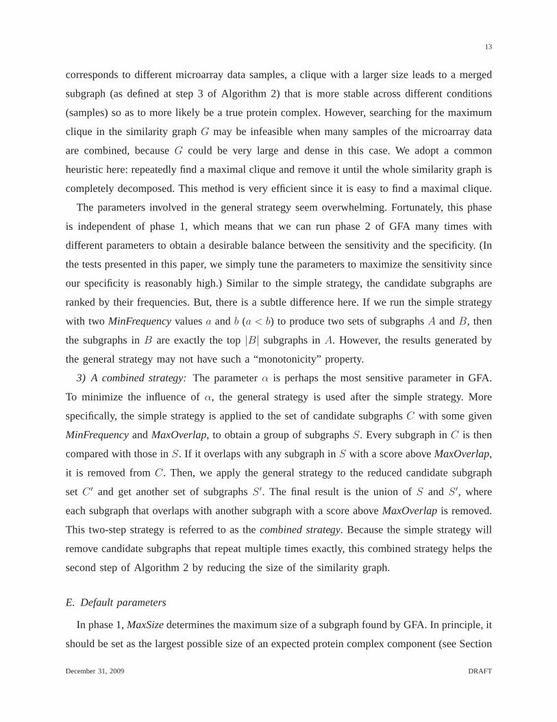
13

corresponds to different microarray data samples, a cliquewith a larger size leads to a merged

subgraph (as defined at step 3 of Algorithm 2) that is more stable across different conditions

(samples) so as to more likely be a true protein complex. However, searching for the maximum

clique in the similarity graphG may be infeasible when many samples of the microarray data

are combined, becauseG could be very large and dense in this case. We adopt a common

heuristic here: repeatedly find a maximal clique and remove it until the whole similarity graph is

completely decomposed. This method is very efficient since it is easy to find a maximal clique.

The parameters involved in the general strategy seem overwhelming. Fortunately, this phase

is independent of phase 1, which means that we can run phase 2 of GFA many times with

different parameters to obtain a desirable balance betweenthe sensitivity and the specificity. (In

the tests presented in this paper, we simply tune the parameters to maximize the sensitivity since

our specificity is reasonably high.) Similar to the simple strategy, the candidate subgraphs are

ranked by their frequencies. But, there is a subtle difference here. If we run the simple strategy

with two MinFrequencyvaluesa andb (a < b) to produce two sets of subgraphsA andB, then

the subgraphs inB are exactly the top|B| subgraphs inA. However, the results generated by

the general strategy may not have such a “monotonicity” property.

3) A combined strategy:The parameterα is perhaps the most sensitive parameter in GFA.

To minimize the influence ofα, the general strategy is used after the simple strategy. More

specifically, the simple strategy is applied to the set of candidate subgraphsC with some given

MinFrequencyandMaxOverlap, to obtain a group of subgraphsS. Every subgraph inC is then

compared with those inS. If it overlaps with any subgraph inS with a score aboveMaxOverlap,

it is removed fromC. Then, we apply the general strategy to the reduced candidate subgraph

set C ′ and get another set of subgraphsS ′. The final result is the union ofS and S ′, where

each subgraph that overlaps with another subgraph with a score aboveMaxOverlapis removed.

This two-step strategy is referred to as thecombined strategy. Because the simple strategy will

remove candidate subgraphs that repeat multiple times exactly, this combined strategy helps the

second step of Algorithm 2 by reducing the size of the similarity graph.

E. Default parameters

In phase 1,MaxSizedetermines the maximum size of a subgraph found by GFA. In principle, it

should be set as the largest possible size of an expected protein complex component (see Section


14

II-A for the definition of protein complex components) for a given PPI network. For example,

in our experiments, for MIPS-PPI, we select 20 as the bound because the maximum size of a

protein complex component in MIPS-MAN-COMP does not exceed 20. Our experiments show

that GFA is quite robust with respect to this parameter sinceits prediction result does not vary

much as long asMaxSizeis sufficiently large. This is especially true when the microarray data

contains many samples, because only the common component ofa group of similar subgraphs

will be found in multiple samples. For example, we also triedsettingMaxSizeas 30 on MIPS-

PPI and observed almost the same result. The parameterMaxIter controls how strictly the size

bound is enforced. A smallMaxIter may lead to output subgraphs with sizes aboveMaxSize.

This property is useful when there are a few protein complexes that are very dense and much

larger than the other protein complexes and we do not want to makeMaxSizetoo large. So, the

parametersMaxSizeandMaxIter together control the sizes of the output subgraphs. According

to our tests, 30 is a sufficiently large value forMaxIter to make sure that the majority (more

than 99.75%) of the output dense subgraphs have sizes belowMaxSize.

For each sliding window, a similarity graph, defined in step 1of Algorithm 2, will be created.

Each clique whose size (i.e., the number of nodes in the clique) aboveMinFrequencyin this

similarity graph corresponds to a merged subgraph. The frequency of each merged subgraph

is defined as the size of its corresponding clique. When more samples are combined, a sliding

window with a certain size may contain more dense subgraphs.Therefore, to use the same

MinFrequency, the sliding window size should be reduced by setting a smaller α when more

samples are combined. In this case, a larger support ratioγ should be used as well. Candidate

subgraphs are ranked according to their frequencies. A largerMinFrequencyleads to more reliable

predictions (see section III).MaxSize, MaxIter andMaxOverlapare independent of the number

of samples used but dependent on the PPI network under study.MaxSizeshould be larger than

the largest size of the expected protein complexes.MaxIter should be large enough to make

GFA break large subgraphs sufficiently small.MaxOverlap is fixed to 0.2 according to [11],

[13], [15].

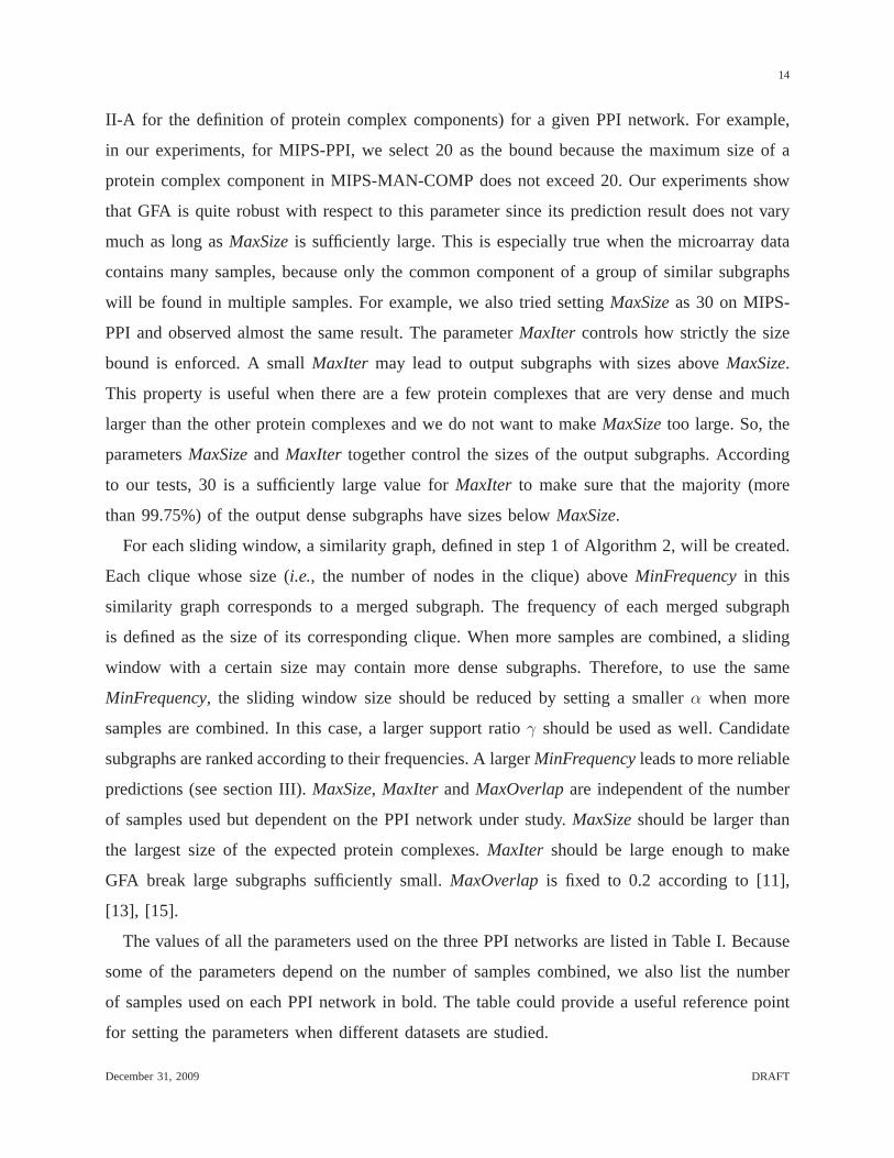
The values of all the parameters used on the three PPI networks are listed in Table I. Because

some of the parameters depend on the number of samples combined, we also list the number

of samples used on each PPI network in bold. The table could provide a useful reference point

for setting the parameters when different datasets are studied.


15

TABLE I

PARAMETER VALUES USED IN OUR EXPERIMENTS

MIPS DIP BioGRID

number of samples 500 600 700

MaxSize 20 30 40

MaxIter 30 30 30

MinFrequency 3 3 3

MaxOverlap 0.2 0.2 0.2

sliding window ratio \ \ 0.2

support ratio \ \ 0.9

The parametersMaxSizeandMaxIter are used in phase 1 of GFA. The parametersMinFrequencyandMaxOverlapare used

in phase 2 by both the simple and general strategies. The parameterssliding window ratioandsupport ratioare used by the

general strategy in phase 2 only.

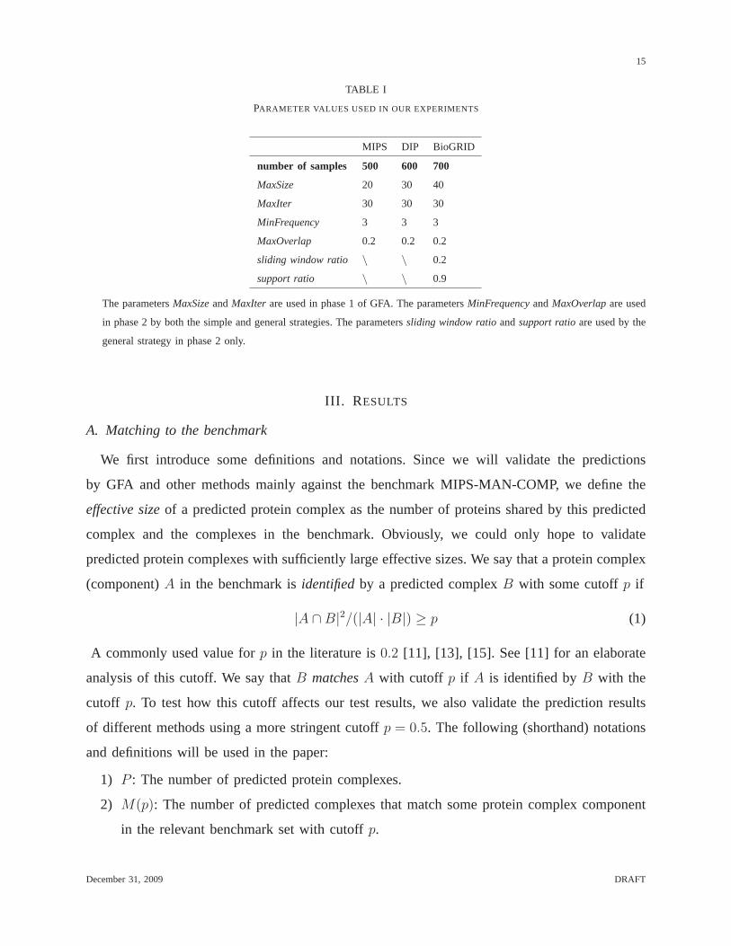
III. R ESULTS

A. Matching to the benchmark

We first introduce some definitions and notations. Since we will validate the predictions

by GFA and other methods mainly against the benchmark MIPS-MAN-COMP, we define the

effective sizeof a predicted protein complex as the number of proteins shared by this predicted

complex and the complexes in the benchmark. Obviously, we could only hope to validate

predicted protein complexes with sufficiently large effective sizes. We say that a protein complex

(component)A in the benchmark isidentifiedby a predicted complexB with some cutoffp if

|A ∩B|2/(|A| · |B|) ≥ p (1)

A commonly used value forp in the literature is0.2 [11], [13], [15]. See [11] for an elaborate

analysis of this cutoff. We say thatB matchesA with cutoff p if A is identified byB with the

cutoff p. To test how this cutoff affects our test results, we also validate the prediction results

of different methods using a more stringent cutoffp = 0.5. The following (shorthand) notations

and definitions will be used in the paper:

1) P : The number of predicted protein complexes.

2) M(p): The number of predicted complexes that match some protein complex component

in the relevant benchmark set with cutoffp.


16

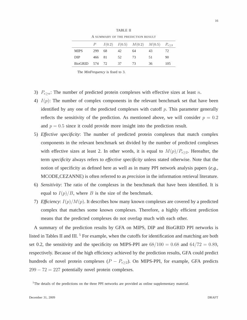
TABLE II

A SUMMARY OF THE PREDICTION RESULT

P I(0.2) I(0.5) M(0.2) M(0.5) Pe≥2

MIPS 299 68 42 64 43 72

DIP 466 81 52 73 51 90

BioGRID 574 72 37 73 36 105

The MinFrequencyis fixed to 3.

3) Pe≥n: The number of predicted protein complexes with effective sizes at leastn.

4) I(p): The number of complex components in the relevant benchmarkset that have been

identified by any one of the predicted complexes with cutoffp. This parameter generally

reflects the sensitivity of the prediction. As mentioned above, we will considerp = 0.2

andp = 0.5 since it could provide more insight into the prediction result.

5) Effective specificity: The number of predicted protein complexes that match complex

components in the relevant benchmark set divided by the number of predicted complexes

with effective sizes at least 2. In other words, it is equal toM(p)/Pe≥2. Hereafter, the

term specificityalways refers toeffective specificityunless stated otherwise. Note that the

notion of specificity as defined here as well as in many PPI network analysis papers (e.g.,

MCODE,CEZANNE) is often referred to asprecisionin the information retrieval literature.

6) Sensitivity: The ratio of the complexes in the benchmark that have been identified. It is

equal toI(p)/B, whereB is the size of the benchmark.

7) Efficiency: I(p)/M(p). It describes how many known complexes are covered by a predicted

complex that matches some known complexes. Therefore, a highly efficient prediction

means that the predicted complexes do not overlap much with each other.

A summary of the prediction results by GFA on MIPS, DIP and BioGRID PPI networks is

listed in Tables II and III.5 For example, when the cutoffs for identification and matching are both

set 0.2, the sensitivity and the specificity on MIPS-PPI are68/100 = 0.68 and 64/72 = 0.89,

respectively. Because of the high efficiency achieved by the prediction results, GFA could predict

hundreds of novel protein complexes (P − Pe≥2). On MIPS-PPI, for example, GFA predicts

299− 72 = 227 potentially novel protein complexes.

5The details of the predictions on the three PPI networks are provided as online supplementary material.


17

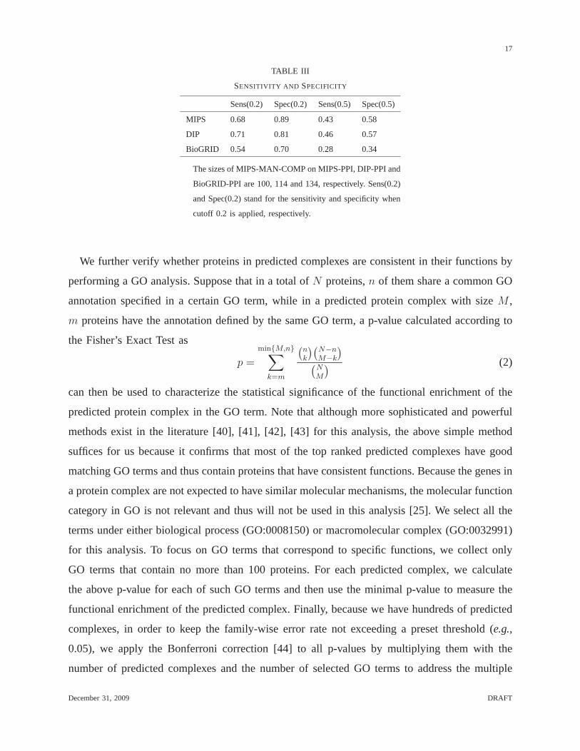
TABLE III

SENSITIVITY AND SPECIFICITY

Sens(0.2) Spec(0.2) Sens(0.5) Spec(0.5)

MIPS 0.68 0.89 0.43 0.58

DIP 0.71 0.81 0.46 0.57

BioGRID 0.54 0.70 0.28 0.34

The sizes of MIPS-MAN-COMP on MIPS-PPI, DIP-PPI and

BioGRID-PPI are 100, 114 and 134, respectively. Sens(0.2)

and Spec(0.2) stand for the sensitivity and specificity when

cutoff 0.2 is applied, respectively.

We further verify whether proteins in predicted complexes are consistent in their functions by

performing a GO analysis. Suppose that in a total ofN proteins,n of them share a common GO

annotation specified in a certain GO term, while in a predicted protein complex with sizeM ,

m proteins have the annotation defined by the same GO term, a p-value calculated according to

the Fisher’s Exact Test as

p =

min{M,n}∑

k=m

(

n

k

)(

N−n

M−k

)

(

N

M

) (2)

can then be used to characterize the statistical significance of the functional enrichment of the

predicted protein complex in the GO term. Note that althoughmore sophisticated and powerful

methods exist in the literature [40], [41], [42], [43] for this analysis, the above simple method

suffices for us because it confirms that most of the top ranked predicted complexes have good

matching GO terms and thus contain proteins that have consistent functions. Because the genes in

a protein complex are not expected to have similar molecularmechanisms, the molecular function

category in GO is not relevant and thus will not be used in thisanalysis [25]. We select all the

terms under either biological process (GO:0008150) or macromolecular complex (GO:0032991)

for this analysis. To focus on GO terms that correspond to specific functions, we collect only

GO terms that contain no more than 100 proteins. For each predicted complex, we calculate

the above p-value for each of such GO terms and then use the minimal p-value to measure the

functional enrichment of the predicted complex. Finally, because we have hundreds of predicted

complexes, in order to keep the family-wise error rate not exceeding a preset threshold (e.g.,

0.05), we apply the Bonferroni correction [44] to all p-values by multiplying them with the

number of predicted complexes and the number of selected GO terms to address the multiple


18

hypothesis testing problem. We further vary the maximum number of proteins allowed in a GO

term (i.e., 50, 75, 100, 125) to assess the impact of this parameter on the analysis, and find that

its impact is negligible. For example, when the predicted complexes on MIPS-PPI are matched

to GO terms under biological process or under macromolecular complex, the percentages of

significant predictions (i.e., those predicted complexes whose corrected p-values for matching

with GO terms under either biological process or macromolecular complex are less than 0.05

when) are 33.1% and 32.8% when the maximum of number of proteins allowed in a GO term

is set to 125 and 50, respectively.

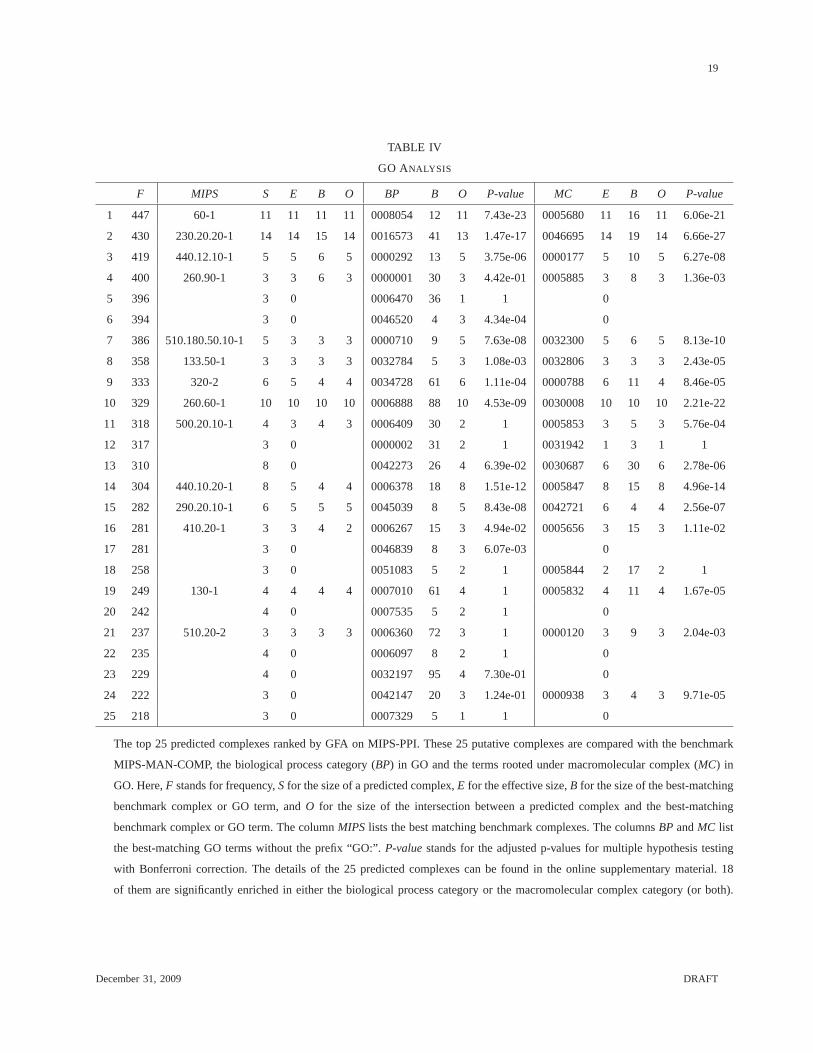
Table IV shows the top 25 predicted complexes with the highest frequencies. From this table,

we can see that many of these putative complexes (e.g., the 1st, 2nd, 3rd, 8th, 10th, 19th and 21th)

match complexes in MIPS-MAN-COMP quite accurately. Besides,they are also functionally

enriched in some GO terms. For predicted complexes that haveno good matches in MIPS-

MAN-COMP (e.g., the 7th and 14th), they are generally enriched in certain GOterms. For

example, the 7th predicted complex contains five proteins (YDR097C, YOL090W, YNL082W,

YMR167W, YCR092C). Only three of them (YCR092C, YNL082W and YOL090W)appear in

MIPS-MAN-COMP and match the complex (component) 510.180.50.10. However, all the five

proteins are members of the “mismatch repair complex” (GO:0032300). In the 14th predicted

complex, all the 8 proteins belong to the mRNA cleavage and polyadenylation specificity factor

complex (GO:0005847). Due to the incompleteness of data in MIPS-MAN-COMP, only 5 of them

appear in MIPS-MAN-COMP and 4 of them match the complex 440.10.20 (pre mRNA3’-end

processing factor CFII) in MIPS. The most interesting group of predicted complexes consists of

those that have zero effective sizes but have strong GO supports. For example, the 6th predicted

complex is totally missed by MIPS-MAN-COMP, but all proteinsin this predicted complex are

involved in the sphingoid biosynthetic process (GO:0046520). In the 13th predicted complex, 6

out of the 8 proteins are ingredients of preribosome (GO:0030687), a precursor of the eukaryotic

cytoplasmic large ribosomal subunit [45]. Finally, the 24th predicted complex matches well with

GARP complex (GO:0000938).

B. Comparison with existing methods

We compare the performance of the proposed GFA algorithm with five existing methods

(jActiveModules [23], MCODE [11], MCL [36], DECAFF[15], and MATISSE [25]) on three


19

TABLE IV

GO ANALYSIS

F MIPS S E B O BP B O P-value MC E B O P-value

1 447 60-1 11 11 11 11 0008054 12 11 7.43e-23 0005680 11 16 11 6.06e-21

2 430 230.20.20-1 14 14 15 14 0016573 41 13 1.47e-17 0046695 14 19 14 6.66e-27

3 419 440.12.10-1 5 5 6 5 0000292 13 5 3.75e-06 0000177 5 10 5 6.27e-08

4 400 260.90-1 3 3 6 3 0000001 30 3 4.42e-01 0005885 3 8 3 1.36e-03

5 396 3 0 0006470 36 1 1 0

6 394 3 0 0046520 4 3 4.34e-04 0

7 386 510.180.50.10-1 5 3 3 3 0000710 9 5 7.63e-08 0032300 5 6 5 8.13e-10

8 358 133.50-1 3 3 3 3 0032784 5 3 1.08e-03 0032806 3 3 3 2.43e-05

9 333 320-2 6 5 4 4 0034728 61 6 1.11e-04 0000788 6 11 4 8.46e-05

10 329 260.60-1 10 10 10 10 0006888 88 10 4.53e-09 0030008 10 10 10 2.21e-22

11 318 500.20.10-1 4 3 4 3 0006409 30 2 1 0005853 3 5 3 5.76e-04

12 317 3 0 0000002 31 2 1 0031942 1 3 1 1

13 310 8 0 0042273 26 4 6.39e-02 0030687 6 30 6 2.78e-06

14 304 440.10.20-1 8 5 4 4 0006378 18 8 1.51e-12 0005847 8 15 8 4.96e-14

15 282 290.20.10-1 6 5 5 5 0045039 8 5 8.43e-08 0042721 6 4 4 2.56e-07

16 281 410.20-1 3 3 4 2 0006267 15 3 4.94e-02 0005656 3 15 3 1.11e-02

17 281 3 0 0046839 8 3 6.07e-03 0

18 258 3 0 0051083 5 2 1 0005844 2 17 2 1

19 249 130-1 4 4 4 4 0007010 61 4 1 0005832 4 11 4 1.67e-05

20 242 4 0 0007535 5 2 1 0

21 237 510.20-2 3 3 3 3 0006360 72 3 1 0000120 3 9 3 2.04e-03

22 235 4 0 0006097 8 2 1 0

23 229 4 0 0032197 95 4 7.30e-01 0

24 222 3 0 0042147 20 3 1.24e-01 0000938 3 4 3 9.71e-05

25 218 3 0 0007329 5 1 1 0

The top 25 predicted complexes ranked by GFA on MIPS-PPI. These 25putative complexes are compared with the benchmark

MIPS-MAN-COMP, the biological process category (BP) in GO and the terms rooted under macromolecular complex (MC) in

GO. Here,F stands for frequency,Sfor the size of a predicted complex,E for the effective size,B for the size of the best-matching

benchmark complex or GO term, andO for the size of the intersection between a predicted complex and the best-matching

benchmark complex or GO term. The columnMIPS lists the best matching benchmark complexes. The columnsBP andMC list

the best-matching GO terms without the prefix “GO:”.P-valuestands for the adjusted p-values for multiple hypothesis testing

with Bonferroni correction. The details of the 25 predicted complexes can be found in the online supplementary material. 18

of them are significantly enriched in either the biological process categoryor the macromolecular complex category (or both).


20

PPI datasets (MIPS, DIP, and BioGRID-PPI). Furthermore, we will compare GFA with two

recent programs CODEC and CEZANNE on the PPI datasets considered in the papers that

introduced the programs [37], [26]. These methods represent the most advanced methods for

predicting protein complexes from PPI and microarray data of a single species.

jActiveModules [23] is one of the first tools that combine PPIand microarray data to find

functional modules. In the comparison, except the number ofmodules returned by jActiveMod-

ules, all parameters of jActiveModules are set to their default values. The number of modules

returned by jActiveModules is set to 1000, the maximum valueallowed, because our tests show

that this value gives jActiveModules the best performance.

MCODE [11] pioneered the method of identifying protein complexes through finding dense

subgraphs in PPI networks. MCL is a clustering algorithm thatuses only PPI information to find

protein complexes [36]. It was found to be the best performerin predicting protein complexes

from PPI data according to the 2006 evaluation study of Broheeand van Helden [46]. A single

parameter,inflation, controls the behavior of MCL. In order to tune the performance of the MCL

algorithm, we perform a grid search by varying this parameter from 1.2 to 5.9 with step size 0.1

(as suggested in [36]) to obtain the optimal value of this parameter that can give us the highest

sensitivity at the identification cutoffp = 0.2. According to our experience, such an optimal

parameter in many cases also leads to reasonably high specificities.

DECAFF [15] is the latest work that uses PPI networks alone to identify protein complexes.

Unfortunately, we have only been able to obtain the results of DECAFF on MIPS-PPI and

BioGRID-PPI, because the program is not available from the authors. Note that the MIPS-PPI

and BioGRID-PPI data used in our studies are the same as those used by DECAFF.

CODEC [37] treats co-immunoprecipitation data as a bipartite graph and identifies dense

subgraphs in the bipartite graph. Note that a co-immunoprecipitation dataset could be considered

as a PPI network by treating each pray-bait relation as an interaction between the pray and the

bait.

MATISSE has five parameters,beta, min seed size, max seed size, min module size, andmax

module size. In our studies, we setbeta to 0.95 as suggested in MATISSE [25], setmin seed

sizeto 2 andmin module sizeto 3 for the purpose of predicting protein complexes that contain

at least 3 proteins, and set bothmax seed sizeandmax module sizeto the defaultMaxSizevalue

in GFA to make the complexes predicted by MATISSE and GFA havecomparable sizes.


21

The programs jActiveModules, CODEC, MATISSE and CEZANNE all use microarray data.

For each PPI dataset, we apply the same subset of microarray samples from GEO used by GFA

to MATISSE. Since we will compare GFA with CODEC and CEZANNE on the datasets in [37],

[26], we will use the reported prediction results of CODEC andCEZANNE instead of running

these programs. jActiveModules requires p-values as computed by another program VERA [47]

for each protein in the input PPI network. However, we were unable to make VERA work for the

GEO microarray dataset or the dataset in [26] because each ofthem is missing some information

required by VERA. Therefore, we use the microarray dataset studied in [47] that contains the

p-values generated by VERA as a part of the input to jActiveModules. Note that the programs

jActiveModules, MATISSE and CEZANNE were not designed to search for protein complexes

specifically.

In addition to these existing methods, we also run GFA with all gene expression values

randomly generated from a uniform(−1, 1) distribution. We call this methodGFA-R and use

it to check the effect of microarray data on the performance of GFA. In our studies, we set

MinFrequencyto 3 for both GFA and GFA-R to ensure highly confident predictions.

In the first group of comparisons, the prediction results of GFA, GFA-R, MCODE, MCL,

DECAFF, and MATISSE on MIPS, DIP and BioGRID-PPI are compared with benchmark

MIPS-MAN-COMP. The performance of each method is evaluated in terms of sensitivity and

specificity. All predicted complexes with fewer than 3 proteins are removed before the calculation

of sensitivity and specificity, because the benchmark contains only complex components of

sizes at least 3. The comparison results are shown in Figure 1. The same set of methods are

also compared using benchmark MIPS-MAN (i.e., the manually curated MIPS complexes that

are not decomposed into connected components) andF-measurewhich was used recently in

[26] to compare various functional module prediction methods. The F-measure is defined as

F = 2∗sensitivity ∗specificity/(sensitivity+specificity). Here, a predicted complex is said

to match a benchmark complex if the corrected p-value (as described in the above GO analysis

section) of matching the two subsets of the proteins contained in the complexes is less than

0.05. 6 Again, a predicted complex is a true positive if it matches some benchmark complex

and a benchmark complex is identified if it has a matching predicted complex. As before, only

6Note that a cutoff of 0.0001 on uncorrected p-values was used in [26].


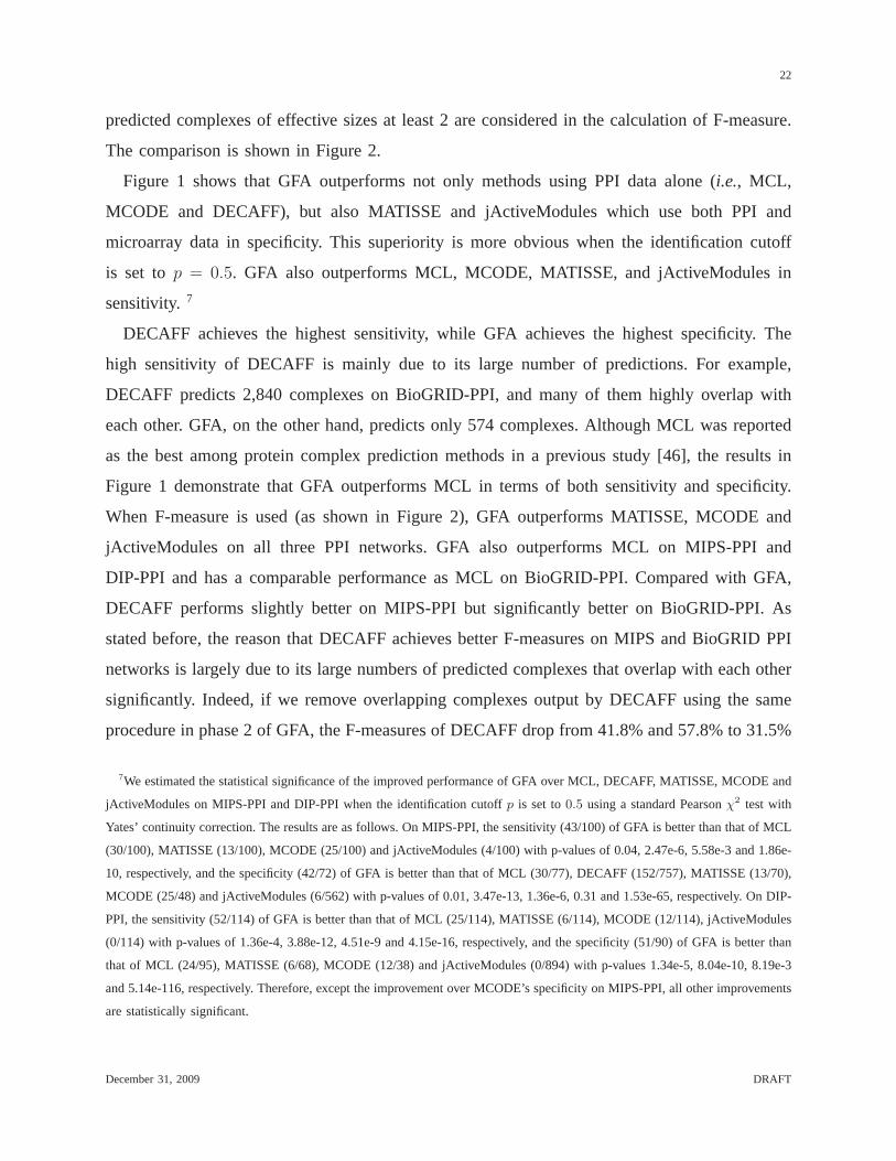
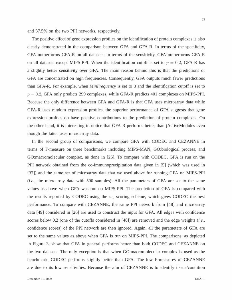
22

predicted complexes of effective sizes at least 2 are considered in the calculation of F-measure.

The comparison is shown in Figure 2.

Figure 1 shows that GFA outperforms not only methods using PPI data alone (i.e., MCL,

MCODE and DECAFF), but also MATISSE and jActiveModules which use both PPI and

microarray data in specificity. This superiority is more obvious when the identification cutoff

is set top = 0.5. GFA also outperforms MCL, MCODE, MATISSE, and jActiveModules in

sensitivity.7

DECAFF achieves the highest sensitivity, while GFA achievesthe highest specificity. The

high sensitivity of DECAFF is mainly due to its large number ofpredictions. For example,

DECAFF predicts 2,840 complexes on BioGRID-PPI, and many of them highly overlap with

each other. GFA, on the other hand, predicts only 574 complexes. Although MCL was reported

as the best among protein complex prediction methods in a previous study [46], the results in

Figure 1 demonstrate that GFA outperforms MCL in terms of bothsensitivity and specificity.

When F-measure is used (as shown in Figure 2), GFA outperformsMATISSE, MCODE and

jActiveModules on all three PPI networks. GFA also outperforms MCL on MIPS-PPI and

DIP-PPI and has a comparable performance as MCL on BioGRID-PPI.Compared with GFA,

DECAFF performs slightly better on MIPS-PPI but significantly better on BioGRID-PPI. As

stated before, the reason that DECAFF achieves better F-measures on MIPS and BioGRID PPI

networks is largely due to its large numbers of predicted complexes that overlap with each other

significantly. Indeed, if we remove overlapping complexes output by DECAFF using the same

procedure in phase 2 of GFA, the F-measures of DECAFF drop from41.8% and 57.8% to 31.5%

7We estimated the statistical significance of the improved performance of GFA over MCL, DECAFF, MATISSE, MCODE and

jActiveModules on MIPS-PPI and DIP-PPI when the identification cutoffp is set to0.5 using a standard Pearsonχ2 test with

Yates’ continuity correction. The results are as follows. On MIPS-PPI, the sensitivity (43/100) of GFA is better than that of MCL

(30/100), MATISSE (13/100), MCODE (25/100) and jActiveModules (4/100) with p-values of 0.04, 2.47e-6, 5.58e-3 and 1.86e-

10, respectively, and the specificity (42/72) of GFA is better than that of MCL (30/77), DECAFF (152/757), MATISSE (13/70),

MCODE (25/48) and jActiveModules (6/562) with p-values of 0.01, 3.47e-13, 1.36e-6, 0.31 and 1.53e-65, respectively. On DIP-

PPI, the sensitivity (52/114) of GFA is better than that of MCL (25/114), MATISSE (6/114), MCODE (12/114), jActiveModules

(0/114) with p-values of 1.36e-4, 3.88e-12, 4.51e-9 and 4.15e-16, respectively, and the specificity (51/90) of GFA is better than

that of MCL (24/95), MATISSE (6/68), MCODE (12/38) and jActiveModules (0/894) with p-values 1.34e-5, 8.04e-10, 8.19e-3

and 5.14e-116, respectively. Therefore, except the improvement over MCODE’s specificity on MIPS-PPI, all other improvements

are statistically significant.


23

and 37.5% on the two PPI networks, respectively.

The positive effect of gene expression profiles on the identification of protein complexes is also

clearly demonstrated in the comparison between GFA and GFA-R. In terms of the specificity,

GFA outperforms GFA-R on all datasets. In terms of the sensitivity, GFA outperforms GFA-R

on all datasets except MIPS-PPI. When the identification cutoff is set to p = 0.2, GFA-R has

a slightly better sensitivity over GFA. The main reason behind this is that the predictions of

GFA are concentrated on high frequencies. Consequently, GFAoutputs much fewer predictions

than GFA-R. For example, whenMinFrequencyis set to 3 and the identification cutoff is set to

p = 0.2, GFA only predicts 299 complexes, while GFA-R predicts 401 complexes on MIPS-PPI.

Because the only difference between GFA and GFA-R is that GFA uses microarray data while

GFA-R uses random expression profiles, the superior performance of GFA suggests that gene

expression profiles do have positive contributions to the prediction of protein complexes. On

the other hand, it is interesting to notice that GFA-R performs better than jActiveModules even

though the latter uses microarray data.

In the second group of comparisons, we compare GFA with CODEC and CEZANNE in

terms of F-measure on three benchmarks including MIPS-MAN,GO:biological process, and

GO:macromolecular complex, as done in [26]. To compare withCODEC, GFA is run on the

PPI network obtained from the co-immunoprecipitation datagiven in [5] (which was used in

[37]) and the same set of microarray data that we used above for running GFA on MIPS-PPI

(i.e., the microarray data with 500 samples). All the parameters of GFA are set to the same

values as above when GFA was run on MIPS-PPI. The prediction of GFA is compared with

the results reported by CODEC using thew1 scoring scheme, which gives CODEC the best

performance. To compare with CEZANNE, the same PPI network from [48] and microarray

data [49] considered in [26] are used to construct the input for GFA. All edges with confidence

scores below 0.2 (one of the cutoffs considered in [48]) are removed and the edge weights (i.e.,

confidence scores) of the PPI network are then ignored. Again, all the parameters of GFA are

set to the same values as above when GFA is run on MIPS-PPI. Thecomparisons, as depicted

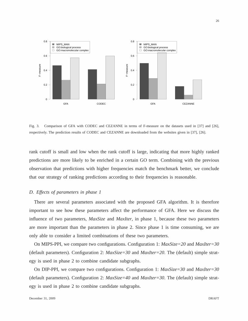
in Figure 3, show that GFA in general performs better than both CODEC and CEZANNE on

the two datasets. The only exception is that when GO:macromolecular complex is used as the

benchmark, CODEC performs slightly better than GFA. The low F-measures of CEZANNE

are due to its low sensitivities. Because the aim of CEZANNE is to identify tissue/condition


24

MIPS DIP BioGRID

Spe

cific

ity &

Sen

sitiv

ity (

0.2)

GFAGFA−RMCLDECAFF

MATISSEMCODEjActiveModules

1

0.5

0

0.5

1

MIPS DIP BioGRID MIPS DIP BioGRID

Spe

cific

ity &

Sen

sitiv

ity (

0.5)

1

0.5

0

0.5

1

GFAGFA−RMCLDECAFF


MIPS DIP BioGRID

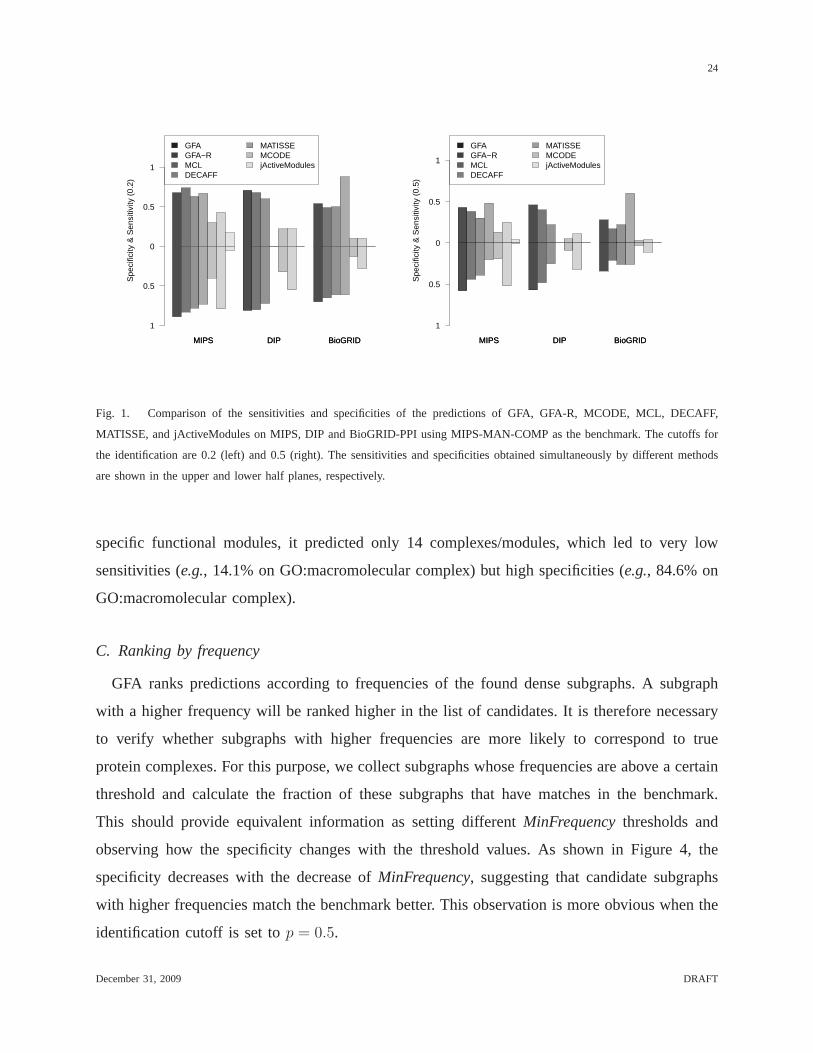
Fig. 1. Comparison of the sensitivities and specificities of the predictions ofGFA, GFA-R, MCODE, MCL, DECAFF,

MATISSE, and jActiveModules on MIPS, DIP and BioGRID-PPI using MIPS-MAN-COMP as the benchmark. The cutoffs for

the identification are 0.2 (left) and 0.5 (right). The sensitivities and specificities obtained simultaneously by different methods

are shown in the upper and lower half planes, respectively.

specific functional modules, it predicted only 14 complexes/modules, which led to very low

sensitivities (e.g., 14.1% on GO:macromolecular complex) but high specificities (e.g., 84.6% on

GO:macromolecular complex).

C. Ranking by frequency

GFA ranks predictions according to frequencies of the founddense subgraphs. A subgraph

with a higher frequency will be ranked higher in the list of candidates. It is therefore necessary

to verify whether subgraphs with higher frequencies are more likely to correspond to true

protein complexes. For this purpose, we collect subgraphs whose frequencies are above a certain

threshold and calculate the fraction of these subgraphs that have matches in the benchmark.

This should provide equivalent information as setting different MinFrequencythresholds and

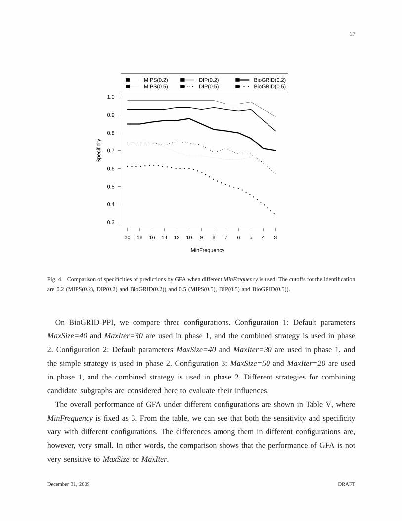
observing how the specificity changes with the threshold values. As shown in Figure 4, the

specificity decreases with the decrease ofMinFrequency, suggesting that candidate subgraphs

with higher frequencies match the benchmark better. This observation is more obvious when the

identification cutoff is set top = 0.5.


25

MIPS DIP BioGRID

F−

mea

sure

GFAGFA−RMCLDECAFF


0

0.2

0.4

0.6

0.8

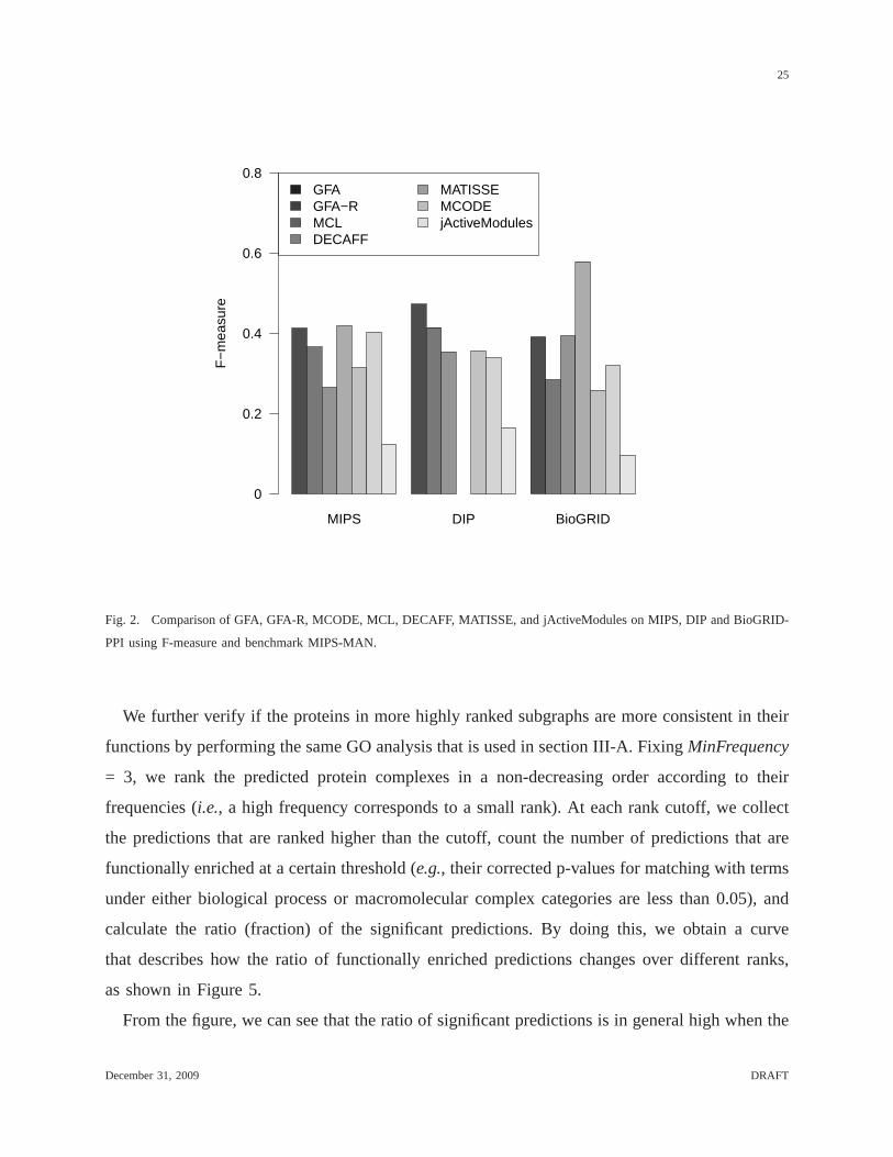
Fig. 2. Comparison of GFA, GFA-R, MCODE, MCL, DECAFF, MATISSE,and jActiveModules on MIPS, DIP and BioGRID-

PPI using F-measure and benchmark MIPS-MAN.

We further verify if the proteins in more highly ranked subgraphs are more consistent in their

functions by performing the same GO analysis that is used in section III-A. Fixing MinFrequency

= 3, we rank the predicted protein complexes in a non-decreasing order according to their

frequencies (i.e., a high frequency corresponds to a small rank). At each rank cutoff, we collect

the predictions that are ranked higher than the cutoff, count the number of predictions that are

functionally enriched at a certain threshold (e.g., their corrected p-values for matching with terms

under either biological process or macromolecular complexcategories are less than 0.05), and

calculate the ratio (fraction) of the significant predictions. By doing this, we obtain a curve

that describes how the ratio of functionally enriched predictions changes over different ranks,

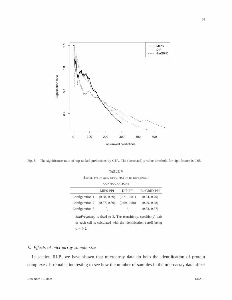
as shown in Figure 5.

From the figure, we can see that the ratio of significant predictions is in general high when the


26

GFA CODEC

F−

mea

sure

MIPS_MANGO:biological processGO:macromolecular complex

0

0.2

0.4

0.6

0.8

GFA CEZANNE

F−

mea

sure

MIPS_MANGO:biological processGO:macromolecular complex

0

0.2

0.4

0.6

0.8

Fig. 3. Comparison of GFA with CODEC and CEZANNE in terms of F-measure on the datasets used in [37] and [26],

respectively. The prediction results of CODEC and CEZANNE are downloaded from the websites given in [37], [26].

rank cutoff is small and low when the rank cutoff is large, indicating that more highly ranked

predictions are more likely to be enriched in a certain GO term. Combining with the previous

observation that predictions with higher frequencies match the benchmark better, we conclude

that our strategy of ranking predictions according to theirfrequencies is reasonable.

D. Effects of parameters in phase 1

There are several parameters associated with the proposed GFA algorithm. It is therefore

important to see how these parameters affect the performance of GFA. Here we discuss the

influence of two parameters,MaxSizeand MaxIter, in phase 1, because these two parameters

are more important than the parameters in phase 2. Since phase 1 is time consuming, we are

only able to consider a limited combinations of these two parameters.

On MIPS-PPI, we compare two configurations. Configuration 1:MaxSize=20andMaxIter=30

(default parameters). Configuration 2:MaxSize=30andMaxIter=20. The (default) simple strat-

egy is used in phase 2 to combine candidate subgraphs.

On DIP-PPI, we compare two configurations. Configuration 1:MaxSize=30andMaxIter=30

(default parameters). Configuration 2:MaxSize=40andMaxIter=30. The (default) simple strat-

egy is used in phase 2 to combine candidate subgraphs.


27

MinFrequency

Spe

cific

ity

20 18 16 14 12 10 9 8 7 6 5 4 3

0.3

0.4

0.5

0.6

0.7

0.8

0.9

1.0

MIPS(0.2)MIPS(0.5)

DIP(0.2)DIP(0.5)

BioGRID(0.2)BioGRID(0.5)

Fig. 4. Comparison of specificities of predictions by GFA when differentMinFrequencyis used. The cutoffs for the identification

are 0.2 (MIPS(0.2), DIP(0.2) and BioGRID(0.2)) and 0.5 (MIPS(0.5), DIP(0.5) and BioGRID(0.5)).

On BioGRID-PPI, we compare three configurations. Configuration1: Default parameters

MaxSize=40and MaxIter=30 are used in phase 1, and the combined strategy is used in phase

2. Configuration 2: Default parametersMaxSize=40and MaxIter=30 are used in phase 1, and

the simple strategy is used in phase 2. Configuration 3:MaxSize=50andMaxIter=20 are used

in phase 1, and the combined strategy is used in phase 2. Different strategies for combining

candidate subgraphs are considered here to evaluate their influences.

The overall performance of GFA under different configurations are shown in Table V, where

MinFrequencyis fixed as 3. From the table, we can see that both the sensitivity and specificity

vary with different configurations. The differences among them in different configurations are,

however, very small. In other words, the comparison shows that the performance of GFA is not

very sensitive toMaxSizeor MaxIter.


28

0 100 200 300 400 500

0.4

0.6

0.8

1.0

Top ranked predictions

Sig

nific

ance

rat

io

MIPSDIPBioGRID

Fig. 5. The significance ratio of top ranked predictions by GFA. The (corrected) p-value threshold for significance is 0.05.

TABLE V

SENSITIVITY AND SPECIFICITY IN DIFFERENT

CONFIGURATIONS

MIPS-PPI DIP-PPI BioGRID-PPI

Configuration 1 (0.68, 0.89) (0.71, 0.81) (0.54, 0.70)

Configuration 2 (0.67, 0.89) (0.69, 0.88) (0.49, 0.68)

Configuration 3 \ \ (0.53, 0.67)

MinFrequencyis fixed to 3. The (sensitivity, specificity) pair

in each cell is calculated with the identification cutoff being

p = 0.2.

E. Effects of microarray sample size

In section III-B, we have shown that microarray data do help the identification of protein

complexes. It remains interesting to see how the number of samples in the microarray data affect


29

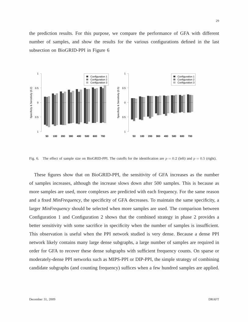
the prediction results. For this purpose, we compare the performance of GFA with different

number of samples, and show the results for the various configurations defined in the last

subsection on BioGRID-PPI in Figure 6

50 100 200 300 400 500 600 700

Spe

cific

ity &

Sen

sitiv

ity (

0.2)

Configuration 1Configuration 2Configuration 3

1

0.5

0

0.5

1

50 100 200 300 400 500 600 700 50 100 200 300 400 500 600 700

Spe

cific

ity &

Sen

sitiv

ity (

0.5)

Configuration 1Configuration 2Configuration 3

1

0.5

0

0.5

1

50 100 200 300 400 500 600 700

Fig. 6. The effect of sample size on BioGRID-PPI. The cutoffs for theidentification arep = 0.2 (left) andp = 0.5 (right).

These figures show that on BioGRID-PPI, the sensitivity of GFA increases as the number

of samples increases, although the increase slows down after 500 samples. This is because as

more samples are used, more complexes are predicted with each frequency. For the same reason

and a fixedMinFrequency, the specificity of GFA decreases. To maintain the same specificity, a

largerMinFrequencyshould be selected when more samples are used. The comparison between

Configuration 1 and Configuration 2 shows that the combined strategy in phase 2 provides a

better sensitivity with some sacrifice in specificity when the number of samples is insufficient.

This observation is useful when the PPI network studied is very dense. Because a dense PPI

network likely contains many large dense subgraphs, a largenumber of samples are required in

order for GFA to recover these dense subgraphs with sufficient frequency counts. On sparse or

moderately-dense PPI networks such as MIPS-PPI or DIP-PPI,the simple strategy of combining

candidate subgraphs (and counting frequency) suffices whena few hundred samples are applied.


30

IV. CONCLUSIONS ANDDISCUSSION

We have presented a max-flow based algorithm, GFA, to identify complexes from PPI networks

by incorporating microarray data. Compared to the previous methods, GFA is actually able to find

the densest subgraphs in the input PPI network efficiently, rather than using some local search

heuristic. Our experiments on the MIPS, DIP and BioGRID PPI networks have demonstrated that

GFA outperforms the previous methods for predicting protein complexes in terms of specificity

while maintaining a comparable sensitivity. Its predictedcomplexes are highly efficient because

they do not overlap much with each other. One of the reasons that GFA was not able to

identify some of the benchmark protein complexes is that it removed nodes of degree 1 from the

network in every iteration. This step is necessary since it prevents GFA from producing many

small spurious predictions. We may have to explore a different strategy in order to improve its

sensitivity.

In phase 1 of GFA, multiple rounds of DSA have to be executed inorder to find a dense

subgraph of a sufficiently small size. This is time consuming. To speed up this step, we can set a

small MaxIter. We have demonstrated that the final result is not very sensitive to this parameter.

An alternative is to assign larger weights to nodes based on expression data in each round.

As mentioned before, GFA uses the multiplying factore−expr(A) to reduce the weights of highly

expressed genes in order to fragment a large dense subgraph.This favors highly expressed genes

and might tend to ignore some of the genes whose expression levels are significantly lower than

their normal levels. A possible solution is to rerun GFA withthe reciprocal multiplying factor

eexpr(A) to favor lowly expressed genes and combine the predicted complexes appropriately with

those obtained with the original multiplying factore−expr(A). We have done some preliminary

testing on this strategy and found that it slightly improvedGFA’s performance on some datasets.

We will investigate the strategy as well as the issue of optimizing the multiplying factor more

carefully in future work.

Our discussion in the previous section shows that the performance of GFA generally improves

when more samples are combined. However, the running time ofGFA is proportional to the

number of samples and could become a concern when the PPI network is large/dense. For

example, in our tests, on MIPS-PPI (500 samples), DIP-PPI (600 samples) and BioGRID-PPI

(700 samples), GFA needs about 4, 15, and 96 hours (the exact running time depends on the


31

parameters used), respectively, on a standard desktop PC. When compared with MCL, MCODE,

and MATISSE, which cost less than one hour on BioGRID-PPI, GFA is much slower. On the

other hand, since phase 1 of GFA (which costs the most time) can be executed independently on

each microarray sample, it is quite straightforward to run GFA in parallel on a computer cluster

to achieve a reasonable speed.

ACKNOWLEDGMENTS

We would like thank the anonymous referees for their many valuable suggestions and com-

ments. This work was partly supported by the Natural ScienceFoundation of China grants

60805010, 60621062, 60503001, 60528001, and 60575014, theHi-Tech Research and Develop-

ment Program of China (863 project) grants 2006AA01Z102 and 2006AA02Z325, NSF grant IIS-

0711129, NIH grant LM008991, Changjiang and Bioinformatics Chair Visiting Professorships

at Tsinghua University.

REFERENCES

[1] P. Uetz, L. Giot, G. Cagney, T. A. Mansfield, R. S. Judson, J. R. Knight, D. Lockshon, V. Narayan, M. Srinivasan,

P. Pochart, A. Qureshi Emili, Y. Li, B. Godwin, D. Conover, T. Kalbfleisch, G. Vijayadamodar, M. Yang, M. Johnston,

S. Fields, and J. M. Rothberg, “A comprehensive analysis of protein-protein interactions in saccharomyces cerevisiae,”

Nature, vol. 403, no. 6770, pp. 623–627, 2000.

[2] T. Ito, K. Tashiro, S. Muta, R. Ozawa, T. Chiba, M. Nishizawa, K. Yamamoto, S. Kuhara, and Y. Sakaki, “Toward a

protein-protein interaction map of the budding yeast: a. comprehensivesystem to examine two-hybrid interactions in all

possible combinations between the yeast proteins,”Proc. Natl Acad. Sci. USA, vol. 97, no. 3, pp. 1143–1147, 2000.

[3] T. Ito, T. Chiba, R. Ozawa, M. Yoshida, M. Hattori, and Y. Sakaki, “A comprehensive two-hybrid analysis to explore the

yeast protein interactome,”Proc. Natl Acad. Sci. USA, vol. 98, no. 8, pp. 4569–4574, 2001.

[4] Y. Ho, A. Gruhler, A. Heilbut, G. D. Bader, L. Moore, S.-L. Adams, A. Millar, P. Taylor, K. Bennett, K. Boutilier,

L. Yang, C. Wolting, I. Donaldson, S. Schandorff, J. Shewnarane,M. Vo, J. Taggart, M. Goudreault, B. Muskat, C. Alfarano,

D. Dewar, Z. Lin, K. Michalickova, A. R. Willems, H. Sassi, P. A. Nielsen,K. J. Rasmussen, J. R. Andersen, L. E. Johansen,

L. H. Hansen, H. Jespersen, A. Podtelejnikov, E. Nielsen, J. Crawford, V. Poulsen, B. D. Sørensen, J. Matthiesen, R. C.

Hendrickson, F. Gleeson, T. Pawson, M. F. Moran, D. Durocher, M. Mann, C. W. V. Hogue, D. Figeys, and M. Tyers,

“Systematic identification of protein complexes in saccharomyces cerevisiae by mass spectrometry,”Nature, vol. 415, no.

6868, pp. 180–183, 2002.

[5] A. C. Gavin, M. Bosche, R. Krause, P. Grandi, M. Marzioch, A. Bauer, J. Schultz, J.M. Rick, A. M. Michon, C. M. Cruciat,

M. Remor, C. Hofert, M. Schelder, M. Brajenovic, H. Ruffner, A. Merino, K. Klein, M. Hudak, D. Dickson, T. Rudi,

V. Gnau, A. Bauch, S. Bastuck, B. Huhse, C. Leutwein, M. A. Heurtier, R. R. Copley, A. Edelmann, E. Querfurth, V. Rybin,

G. Drewes, M. Raida, T. Bouwmeester, P. Bork, B. Seraphin, B. Kuster, G. Neubauer, and G. Superti Furga, “Functional

organization of the yeast proteome by systematic analysis of protein complexes,”Nature, vol. 415, no. 6868, pp. 141–147,

2002.


32

[6] L. Salwinski, C. S. Miller, A. J. Smith, F. K. Pettit, J. U. Bowie, and D. Eisenberg, “The database of interacting proteins:

2004 update,”Nucleic Acids Research, vol. 32, no. Database issue, pp. D449–D451, 2004.

[7] U. Guldener, M. Munsterkotter, G. Kastenmuller, N. Strack, J. v. Helden, C. Lemer, J. Richelles, S. J. Wodak, J.Garcıa-

Martınez, J. E. Perez-Ortın, H. Michael, A. Kaps, E. Talla, B. Dujon, B. Andre, J. L. Souciet, J. D. Montigny, E. Bon,

C. Gaillardin, and H. W. Mewes, “CYGD: the comprehensive yeast genome database,”Nucleic Acids Research, vol. 33,

no. Database issue, pp. D364–D368, 2005.

[8] C. Stark, B. J. Breitkreutz, T. Reguly, L. Boucher, A. Breitkreutz, and M. Tyers, “BioGRID: a. general repository for

interaction datasets,”Nucleic Acids Research, vol. 34, no. Database issue, pp. D535–D539, 2006.

[9] U. Stelzl, U. Worm, M. Lalowski, C. Haenig, F. H. Brembeck, H. Goehler, M. Stroedicke, M. Zenkner, A. Schoenherr,

S. Koeppen, J. Timm, S. Mintzlaff, C. Abraham, N. Bock, S. Kietzmann, A. Goedde, E. Toksoz, A. Droege, S. Krobitsch,

B. Korn, et al., “A human protein-protein interaction network: A resource for annotating the proteome,”Cell, vol. 122,

no. 6, pp. 957–968, 2005.

[10] T. Barrett, D. B. Troup, S. E. Wilhite, P. Ledoux, D. Rudnev, C. Evangelista, I. F. Kim, A. Soboleva, M. Tomashevsky,

and R. Edgar, “NCBI GEO: mining tens of millions of expression profiles–database and tools update,”Nucleic Acids

Research, vol. 35, no. Database issue, pp. D760–D765, 2007.

[11] G. D. Bader and C. W. V. Hogue, “An automated method for findingmolecular complexes in large protein interaction

networks,”BMC Bioinformatics, vol. 4, no. 2, 2003.

[12] V. Spirin and L. A. Mirny, “Protein complexes and functional modules in molecular networks,”Proc. Natl Acad. Sci. USA,

vol. 100, no. 21, pp. 12 123–12 128, 2003.

[13] P. J. Pei and A. D. Zhang, “A ’seed-refine’ algorithm for detecting protein complexes from protein interaction data,”IEEE

Transactions on Nanobioscience, vol. 6, no. 1, pp. 43–50, 2007.

[14] X. L. Li, S. H. Tan, C. S. Foo, and S. K. Ng, “Interaction graph mining for protein complexes using local clique merging,”

Genome Informatics, vol. 16, no. 2, pp. 260–269, 2005.

[15] X. L. Li, C. S. Foo, and S. K. Ng, “Discovering protein complexesin dense reliable neighborhoods of protein interaction

networks,”Comput. Syst. Bioinformatics Conf., vol. 6, pp. 157–168, 2007.

[16] A. H. Y. Tong, B. Drees, G. Nardelli, G. D. Bader, B. Brannetti, L. Castagnoli, M. Evangelista, S. Ferracuti, B. Nelson,

S. Paoluzi, M. Quondam, A. Zucconi, C. W. V. Hogue, S. Fields, C. Boone, and G. Cesareni, “A combined experimental

and computational strategy to dene protein interaction networks for peptiderecognition modules,”Science, vol. 295, no.

5553, pp. 321–324, 2002.

[17] B. Andreopoulos, A. An, X. Wang, M. Faloutsos, and M. Schroeder, “Clustering by common friends finds locally significant

proteins mediating modules,”Bioinformatics, vol. 23, no. 9, pp. 1124–1131, 2007.

[18] A. D. King, N. Przulj, and I. Jurisica, “Protein complex prediction via cost-based clustering,” Bioinformatics, vol. 20,

no. 17, pp. 3013–3020, 2004.

[19] D. Bu, Y. Zhao, L. Cai, H. Xue, X. Zhu, H. Lu, J. Zhang, S. Sun, L. Ling, N. Zhang, G. Li, and R. Chen, “Topological

structure analysis of the protein-protein interaction network in budding yeast,” Nucleic Acids Research, vol. 31, no. 9, pp.

2443–2450, 2003.

[20] C. Wang, C. Ding, Q. Yang, and S. R. Holbrook, “Consistent dissection of the protein interaction network by combining

global and local metrics,”Genome Biology, vol. 8, no. 12, p. R271, 2007.

[21] E. Segal, H. Wang, and D. Koller, “Discovering molecular pathways from protein interaction and gene expression data,”

Bioinformatics, vol. 19, no. Suppl 1, pp. i264–272, 2003.


33

[22] J. Chen and B. Yuan, “Detecting functional modules in the yeast protein-protein interaction network,”Bioinformatics,

vol. 22, no. 18, pp. 2283–2290, 2006.

[23] T. Ideker, O. Ozier, B. Schwikowski, and A. F. Siegel, “Discovering regulatory and signalling circuits in molecular

interaction networks,”Bioinformatics, vol. 18, no. Suppl 1, pp. S233–S240, 2002.

[24] Z. Guo, Y. Li, X. Gong, C. Yao, W. Ma, D. Wang, Y. Li, J. Zhu, M.Zhang, D. Yang, and J. Wang, “Edge-based scoring

and searching method for identifying condition-responsive protein-protein interaction sub-network,”Bioinformatics, vol. 23,

no. 16, pp. 2121–2128, 2007.

[25] I. Ulitsky and R. Shamir, “Identification of functional modules usingnetwork topology and high-throughput data,”BMC

Syst Biol., vol. 1, no. 8, 2007.

[26] ——, “Identifying functional modules using expression profiles and confidence-scored protein interactions,”Bioinformatics,

vol. 25, no. 9, pp. 1158–1164, 2009.

[27] R. Jansen, D. Greenbaum, and M. Gerstein, “Relating whole-genome expression data with protein-protein interactions,”

Genome Res, vol. 12, no. 1, pp. 37–46, 2002.

[28] N. Simonis, D. Gonze, C. Orsi, J. v. Helden, and S. J. Wodak, “Modularity of the transcriptional response of protein

complexes in yeast,”Journal of Molecular Biology, vol. 363, no. 2, pp. 589–610, 2006.

[29] S. Tornow and H. W. Mewes, “Functional modules by relating protein interaction networks and gene expression,”Nucleic

Acids Research, vol. 31, no. 21, pp. 6283–6289, 2003.

[30] R. Sharan, T. Ideker, B. P. Kelley, R. Shamir, and R. M. Karp,“Identification of protein complexes by comparative analysis

of yeast and bacterial protein interaction data,”J. Comput. Biol, vol. 12, no. 6, pp. 835–846, 2005.

[31] E. Hirsh and R. Sharan, “Identification of conserved protein complexes based on a model of protein network evolution,”

Bioinformatics, vol. 23, no. 2, pp. e170–e176, 2007.

[32] J. Flannick, A. Novak, B. S. Srinivasan, H. H. McAdams, and S. Batzoglou, “Graemlin: general and robust alignment of

multiple large interaction networks.”Genome Res, vol. 16, no. 9, pp. 1169–1181, 2006.

[33] R. Sharan and T. Ideker, “Modeling cellular machinery through biological network comparison,”Nat Biotech, vol. 24,

no. 4, pp. 427–433, 2006.

[34] Z. Li, S. Zhang, Y. Wang, X. S. Zhang, and L. Chen, “Alignmentof molecular networks by integer quadratic programming,”

Bioinformatics, vol. 23, no. 13, pp. 1631–1639, 2007.

[35] G. Gallo, M. D. Grigoriadis, and R. E. Tarjan, “A fast parametric maximum flow algorithm and applications,”SIAM J.

Comput, vol. 18, no. 1, pp. 30–55, 1989.

[36] S. van Dongen, Ph.D. dissertation, University of Utrecht, 2000.

[37] G. Geva and R. Sharan, “ Identification of protein complexes fromco-immunoprecipitation data,”unpublished manuscript,

2008.

[38] The Gene Ontology Consortium, “Gene ontology: tool for the unification of biology,” Nat Genet, vol. 25, no. 1, pp. 25–29,

2000.

[39] M. R. Garey and D. S. Johnson,Computers and intractability : a guide to the theory of NP-completeness. W. H. Freeman,

1979.

[40] S. Bauer, S. Grossmann, M. Vingron, and P. N. Robinson, “Ontologizer 2.0–a multifunctional tool for GO term enrichment

analysis and data exploration,”Bioinformatics, vol. 24, no. 14, pp. 1650–1651, 2008.

[41] T. Beissbarth and T. P. Speed, “Gostat: find statistically overrepresented gene ontologies within a group of genes,”

Bioinformatics, vol. 20, no. 9, pp. 1464–1465, 2004.


34

[42] S. Zhong, K. F. Storch, O. Lipan, M. C. J. Kao, C. J. Weitz, and W. H. Wong, “Gosurfer: a graphical interactive tool for

comparative analysis of large gene sets in gene ontology space,”Appl. Bioinformatics, vol. 3, no. 4, pp. 261–264, 2004.

[43] R. Shamir, A. Maron Katz, A. Tanay, C. Linhart, I. Steinfeld, R. Sharan, Y. Shiloh, and R. Elkon, “Expander–an integrative

program suite for microarray data analysis.”BMC Bioinformatics, vol. 6, no. 232, 2005.

[44] R. G. Miller, Simultaneous statistical inference, 2nd ed. Springer Verlag, 1981.

[45] D. Kressler, P. Linder, and J. d. l. Cruz, “Protein trans-acting factors involved in ribosome biogenesis in saccharomyces

cerevisiae,”Mol Cell Biol., vol. 19, no. 12, pp. 7897–7912, 1999.

[46] S. Brohee and J. v. Helden, “Evaluation of clustering algorithms for protein-protein interaction networks,”BMC

Bioinformatics, vol. 7, no. 488, 2006.

[47] T. Ideker, V. Thorsson, A. F. Siegel, and L. E. Hood, “Testingfor differentially-expressed genes by maximum-likelihood

analysis of microarray data,”Journal of Computational Biology, vol. 7, no. 6, pp. 805–817, 2000.

[48] S. R. Collins, P. Kemmeren, X.-C. Zhao, J. F. Greenblatt, F. Spencer, F. C. P. Holstege, J. S. Weissman, and N. J. Krogan,

“Toward a Comprehensive Atlas of the Physical Interactome of Saccharomyces cerevisiae,”Mol Cell Proteomics, vol. 6,

no. 3, pp. 439–450, 2007.

[49] A. P. Gasch, M. Huang, S. Metzner, D. Botstein, S. J. Elledge, and P. O. Brown, “Genomic Expression Responses to

DNA-damaging Agents and the Regulatory Role of the Yeast ATR Homolog Mec1p,”Mol. Biol. Cell, vol. 12, no. 10, pp.

2987–3003, 2001.


Documents

1 A Max-Flow Based Approach to the Identiï¬cation of Protein