1

A Deep Structured Learning Approach TowardsAutomating Connectome Reconstruction from

3D Electron MicrographsJan Funke?, Fabian David Tschopp?, William Grisaitis, Arlo Sheridan,

Chandan Singh, Stephan Saalfeld, Srinivas C. Turaga

F

Abstract—We present a deep structured learning method for neuronsegmentation from 3D electron microscopy (EM) which improves signif-icantly upon the state of the art in terms of accuracy and scalability. Ourmethod consists of a 3D U-NET architecture, trained to predict affinitygraphs on voxels, followed by a simple and efficient iterative regionagglomeration. We train the U-NET using a new structured loss functionbased on MALIS that encourages topological correctness. Our MALIS ex-tension consists of two parts: First, we present an O(n log(n))method tocompute the loss gradient, which improves over the originally proposedO(n2) algorithm. Second, we compute the gradient in two separatepasses to avoid spurious gradient contributions in early training stages.Our affinity predictions are accurate enough that simple learning-freepercentile-based agglomeration outperforms more involved methodsused earlier on inferior predictions. We present results on three EMdatasets (CREMI, FIB-25, and SEGEM) of different imaging techniquesand animals where we achieve relative improvements over previousresults of 27%, 15%, and 250%, respectively. Our findings suggestthat a single 3D segmentation strategy can be applied to both nearlyisotropic block-face EM data and anisotropic serial sectioned EM data.The runtime of our method scales with O(n) in the size of the volume andachieves a throughput of about 2.6 seconds per megavoxel, qualifyingour method for the processing of very large datasets.

1 INTRODUCTION

Precise reconstruction of neural connectivity is of greatimportance to understand the function of biological nervoussystems. 3D electron microscopy (EM) is the only availableimaging method with the resolution necessary to visualizeand reconstruct dense neural morphology without ambi-guity. At this resolution, however, even moderately smallneural circuits yield image volumes that are too large formanual reconstruction. Therefore, automated methods forneuron tracing are needed to aid human analysis.

We present a structured deep learning based image seg-mentation method for reconstructing neurons from 3D elec-tron microscopy which improves significantly upon state ofthe art in terms of accuracy and scalability. For an overview,see Fig. 1, top row. The main components of our methodare: (1) Prediction of 3D affinity graphs using a 3D U-NETarchitecture [1], (2) a structured loss based on MALIS [2] totrain the U-NET to minimize topological errors, and (3) an

? these authors contributed equally

efficient O(n) agglomeration scheme based on quantiles ofpredicted affinities.

The choice of using a 3D U-NET architecture to predictvoxel affinities is motivated by two considerations: First,U-NETs have already shown superior performance on thesegmentation of 2D [3] and 3D [1] biomedical image data.One of their favourable properties is the multi-scale architec-ture which enables computational and statistical efficiency.Second, U-NETs efficiently predict large regions. This isof particular interest in combination with training on theMALIS structured loss, for which we need affinity predic-tions in a region.

We train our 3D U-NET to predict affinities using anextension of the MALIS loss function [2]. Like the originalMALIS loss, we minimize a topological error on hypotheti-cal thresholding and connected component analysis on thepredicted affinities. We extended the original formulation toderive the gradient with respect to all predicted affinities (asopposed to sparsely sampling them), leading to denser andfaster gradient computation. Furthermore, we compute theMALIS loss in two passes: In the positive pass, we constrainall predicted affinities between and outside of ground-truthregions to be 0, and in the negative pass, we constrain affini-ties inside regions to be 1 which avoids spurious gradientsin early training stages.

Although the training is performed assuming subse-quent thresholding, we found iterative agglomeration offragments (or “supervoxels”) to be more robust to smallerrors in the affinity predictions. To this end, we extractfragments running a watershed algorithm on the predictedaffinities. The fragments are then represented in a regionadjacency graph (RAG), where edges are scored to reflectthe predicted affinities between adjacent fragments: edgeswith small scores will be merged before edges with highscores. We discretize edge scores into k evenly distributedbins, which allows us to use a bucket priority queue forsorting. This way, the agglomeration can be carried out witha worst-case linear runtime.

The resulting method (prediction of affinities, watershed,and agglomeration) scales favourably with O(n) in the sizen of the volume, a crucial property for neuron segmentationfrom EM volumes, where volumes easily reach several

arX

iv:1

709.

0297

4v3

[cs

.CV

] 2

4 Se

p 20

17

2

3D U-NET

+ MALIS

seededwatershed

percentile ag-glomeration

raw volume affinities oversegmentation final seg-mentation

(a) 3D U-NET.

AB

C

x

y z50nm

(b) Inter-voxel affinities.

A B C D

C DA

CA

a b c

d e

cb

e

b

[a,d,c,b,e]

[d,c,b,e]

[b,e]

b,d→ b

b,e→ b

A

B

C

D

AC

D

A C

thre

shol

d

segmentation RAG and merge hierarchy queue

(c) Percentile agglomeration.

Figure 1: Overview of our method (top row). Using a 3D U-NET (a), trained with the proposed constrained MALIS loss,we directly predict inter-voxel affinities from volumes of raw data. Affinities provide advantages especially in the case oflow-resolution data (b). In the example shown here, the voxels cannot be labeled correctly as foreground/background: If Awere labeled as foreground, it would necessarily merge with the regions in the previous and next section. If it were labeledas background, it would introduce a split. The labeling of affinities on edges allows B and C to separate A from adjacentsections, while maintaining connectivity inside the region. From the predicted affinities, we obtain an over-segmentationthat is then merged into the final segmentation using a percentile-based agglomeration algorithm (c).

hundreds of terabytes. This is a major advantage overcurrent state-of-the-art methods that all follow a similarpattern. First, voxel-wise predictions are made using adeep neural network. Subsequently, fragments are obtainedfrom these predictions which are then merged using eithergreedy (CELIS [4], GALA [5]) or globally optimal objectives(MULTICUT [6] and lifted MULTICUT [7], [8]). Current ef-forts focus mostly on the merging of fragments: Both CELISand GALA train a classifier to predict scores for hierarchicalagglomeration which increases the computational complex-ity of agglomeration during inference. Similarly, the MUL-TICUT variants train a classifier to predict the connectivityof fragments that are then clustered by solving a compu-tationally expensive combinatorial optimization problem.Our proposed fragment agglomeration method drasticallyreduces the computation complexity compared to previousmerge methods and does not require a separate trainingstep.

We demonstrate the efficacy of our method on three di-verse datasets of EM volumes, imaged by three different 3Delectron microscopy techniques: CREMI (ssTEM, Drosophila),FIB-25 (FIBSEM, Drosophila), and SEGEM (SBEM, mousecortex). Our method significantly improves over the current

state of the art in each of these datasets, outperforming inparticular computationally more expensive methods with-out favorable worst-case runtime guarantees.

We made the source code for training1 and agglomera-tion2 publicly available, together with usage example scriptsto reproduce our CREMI results3.

2 METHOD

2.1 Deep multi-scale convolutional network for predict-ing 3D voxel affinitiesWe use a 3D U-NET architecture [1] to predict voxel affini-ties on 3D volumes. We use the same architecture for allinvestigated datasets which we illustrate in Fig. 1a. In par-ticular, our 3D U-NET consists of four levels of differentresolutions. In each level, we perform at least one convo-lution pass (shown as blue arrows in Fig. 1a) consisting oftwo convolutions (kernel size 3×3×3) followed by rectifiedlinear units. Between the levels, we perform max poolingon variable kernel sizes depending on the dataset resolution

1. https://github.com/naibaf7/caffe2. https://github.com/funkey/waterz3. http://cremi.org/static/data/20170312 mala v2.tar.gz

3

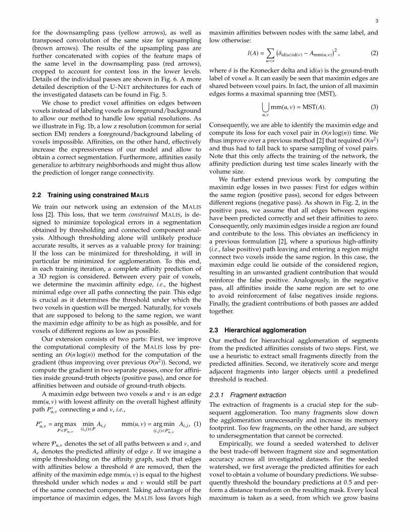
for the downsampling pass (yellow arrows), as well astransposed convolution of the same size for upsampling(brown arrows). The results of the upsampling pass arefurther concatenated with copies of the feature maps ofthe same level in the downsampling pass (red arrows),cropped to account for context loss in the lower levels.Details of the individual passes are shown in Fig. 6. A moredetailed description of the U-NET architectures for each ofthe investigated datasets can be found in Fig. 5.

We chose to predict voxel affinities on edges betweenvoxels instead of labeling voxels as foreground/backgroundto allow our method to handle low spatial resolutions. Aswe illustrate in Fig. 1b, a low z resolution (common for serialsection EM) renders a foreground/background labeling ofvoxels impossible. Affinities, on the other hand, effectivelyincrease the expressiveness of our model and allow toobtain a correct segmentation. Furthermore, affinities easilygeneralize to arbitrary neighborhoods and might thus allowthe prediction of longer range connectivity.

2.2 Training using constrained MALIS

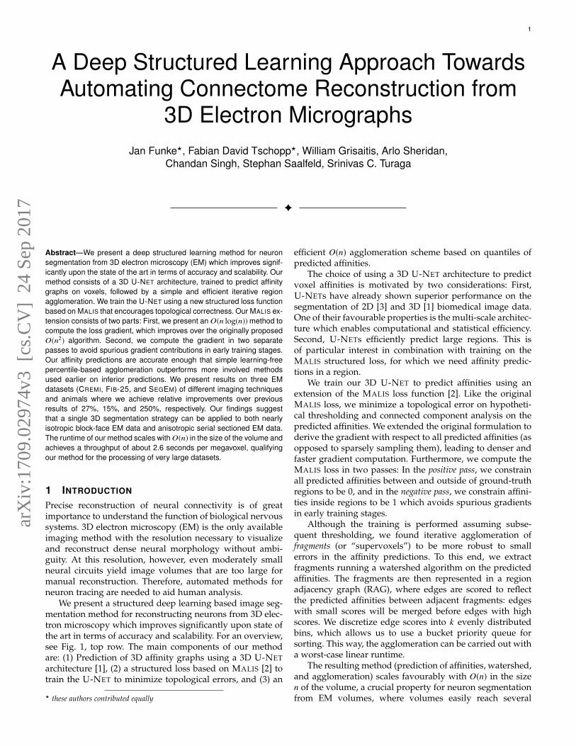
We train our network using an extension of the MALISloss [2]. This loss, that we term constrained MALIS, is de-signed to minimize topological errors in a segmentationobtained by thresholding and connected component anal-ysis. Although thresholding alone will unlikely produceaccurate results, it serves as a valuable proxy for training:If the loss can be minimized for thresholding, it will inparticular be minimized for agglomeration. To this end,in each training iteration, a complete affinity prediction ofa 3D region is considered. Between every pair of voxels,we determine the maximin affinity edge, i.e., the highestminimal edge over all paths connecting the pair. This edgeis crucial as it determines the threshold under which thetwo voxels in question will be merged. Naturally, for voxelsthat are supposed to belong to the same region, we wantthe maximin edge affinity to be as high as possible, and forvoxels of different regions as low as possible.

Our extension consists of two parts: First, we improvethe computational complexity of the MALIS loss by pre-senting an O(n log(n)) method for the computation of thegradient (thus improving over previous O(n2)). Second, wecompute the gradient in two separate passes, once for affini-ties inside ground-truth objects (positive pass), and once foraffinities between and outside of ground-truth objects.

A maximin edge between two voxels u and v is an edgemm(u, v) with lowest affinity on the overall highest affinitypath P∗u,v connecting u and v, i.e.,

P∗u,v = arg maxP∈Pu,v

min(i, j)∈P

Ai, j mm(u, v) = arg min(i, j)∈P∗u,v

Ai, j , (1)

where Pu,v denotes the set of all paths between u and v, andAe denotes the predicted affinity of edge e. If we imagine asimple thresholding on the affinity graph, such that edgeswith affinities below a threshold θ are removed, then theaffinity of the maximin edge mm(u, v) is equal to the highestthreshold under which nodes u and v would still be partof the same connected component. Taking advantage of theimportance of maximin edges, the MALIS loss favors high

maximin affinities between nodes with the same label, andlow otherwise:

l(A) =∑u<v

(δid(u) id(v) − Amm(u,v)

)2 , (2)

where δ is the Kronecker delta and id(u) is the ground-truthlabel of voxel u. It can easily be seen that maximin edges areshared between voxel pairs. In fact, the union of all maximinedges forms a maximal spanning tree (MST),⋃

u,v

mm(u, v) =MST(A). (3)

Consequently, we are able to identify the maximin edge andcompute its loss for each voxel pair in O(n log(n)) time. Wethus improve over a previous method [2] that required O(n2)and thus had to fall back to sparse sampling of voxel pairs.Note that this only affects the training of the network, theaffinity prediction during test time scales linearly with thevolume size.

We further extend previous work by computing themaximin edge losses in two passes: First for edges withinthe same region (positive pass), second for edges betweendifferent regions (negative pass). As shown in Fig. 2, in thepositive pass, we assume that all edges between regionshave been predicted correctly and set their affinities to zero.Consequently, only maximin edges inside a region are foundand contribute to the loss. This obviates an inefficiency ina previous formulation [2], where a spurious high-affinity(i.e., false positive) path leaving and entering a region mightconnect two voxels inside the same region. In this case, themaximin edge could lie outside of the considered region,resulting in an unwanted gradient contribution that wouldreinforce the false positive. Analogously, in the negativepass, all affinities inside the same region are set to oneto avoid reinforcement of false negatives inside regions.Finally, the gradient contributions of both passes are addedtogether.

2.3 Hierarchical agglomeration

Our method for hierarchical agglomeration of segmentsfrom the predicted affinities consists of two steps. First, weuse a heuristic to extract small fragments directly from thepredicted affinities. Second, we iteratively score and mergeadjacent fragments into larger objects until a predefinedthreshold is reached.

2.3.1 Fragment extractionThe extraction of fragments is a crucial step for the sub-sequent agglomeration. Too many fragments slow downthe agglomeration unnecessarily and increase its memoryfootprint. Too few fragments, on the other hand, are subjectto undersegmentation that cannot be corrected.

Empirically, we found a seeded watershed to deliverthe best trade-off between fragment size and segmentationaccuracy across all investigated datasets. For the seededwatershed, we first average the predicted affinities for eachvoxel to obtain a volume of boundary predictions. We subse-quently threshold the boundary predictions at 0.5 and per-form a distance transform on the resulting mask. Every localmaximum is taken as a seed, from which we grow basins

4

0.165992841527790.73812714085827

0.684497336430710.14125302771165

0.650025690183990.72731170483274

0.27272447616454

0.160331126237440.6049847870157

0.172998541813810.25307619644007

0.163572052616430.62714567856265

0.62134905160468

0.752134314436530.1163344565855

0.210191241703090.21293037781163

0.748654101392560.79635202996263

0.64376995863568

0.6908791841431

0.7037308046146

0.71476834561432

A

B

C

0

1

(a) Predicted affinities.

0.165992841527790.73812714085827

0.684497336430710

00

0.27272447616454

00.6049847870157

00

00

0.62134905160468

0.752134314436530

00

0.748654101392560.79635202996263

0.64376995863568

0.6908791841431

0

0.71476834561432

0

1

(b) Positive pass.

11

10.14125302771165

0.650025690183990.72731170483274

1

0.160331126237441

0.172998541813810.25307619644007

0.163572052616430.62714567856265

1

10.1163344565855

0.210191241703090.21293037781163

11

1

1

0.7037308046146

1

0

1

(c) Negative pass.

0.261872859141730.31550266356929

-0.65002569018399-0.72731170483274

0.72727552383546

0.3950152129843

-0.25307619644007

0.37865094839532

0.24786568556347

-0.212930377811630.25134589860744

0.20364797003737

0.3091208158569

-0.7037308046146

0.28523165438568

A

B

C

-

+

(d) Gradient of loss.

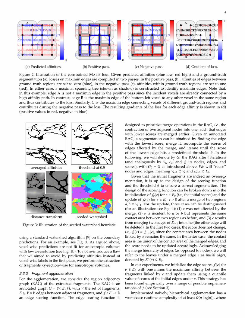
Figure 2: Illustration of the constrained MALIS loss. Given predicted affinities (blue low, red high) and a ground-truthsegmentation (a), losses on maximin edges are computed in two passes: In the positive pass, (b), affinities of edges betweenground-truth regions are set to zero (blue), in the negative pass (c), affinities within ground-truth regions are set to one(red). In either case, a maximal spanning tree (shown as shadow) is constructed to identify maximin edges. Note that,in this example, edge A is not a maximin edge in the positive pass since the incident voxels are already connected by ahigh affinity path. In contrast, edge B is the maximin edge of the bottom left voxel to any other voxel in the same regionand thus contributes to the loss. Similarly, C is the maximin edge connecting voxels of different ground-truth regions andcontributes during the negative pass to the loss. The resulting gradients of the loss for each edge affinity is shown in (d)(positive values in red, negative in blue).

averaged affinities threshold at 0.5

distance transform seeded watershed

Figure 3: Illustration of the seeded watershed heuristic.

using a standard watershed algorithm [9] on the boundarypredictions. For an example, see Fig. 3. As argued above,voxel-wise predictions are not fit for anisotropic volumeswith low z-resolution (see Fig. 1b). To not re-introduce a flawthat we aimed to avoid by predicting affinities instead ofvoxel-wise labels in the first place, we perform the extractionof fragments xy-section-wise for anisotropic volumes.

2.3.2 Fragment agglomerationFor the agglomeration, we consider the region adjacencygraph (RAG) of the extracted fragments. The RAG is anannotated graph G = (V, E, f ), with V the set of fragments,E ⊆ V ×V edges between adjacent fragments, and f : E 7→ Ran edge scoring function. The edge scoring function is

designed to prioritize merge operations in the RAG, i.e., thecontraction of two adjacent nodes into one, such that edgeswith lower scores are merged earlier. Given an annotatedRAG, a segmentation can be obtained by finding the edgewith the lowest score, merge it, recompute the scores ofedges affected by the merge, and iterate until the scoreof the lowest edge hits a predefined threshold θ. In thefollowing, we will denote by Gi the RAG after i iterations(and analogously by Vi , Ei , and fi its nodes, edges, andscores), with G0 = G as introduced above. We will ”reuse”nodes and edges, meaning Vi+1 ⊂ Vi and Ei+1 ⊂ Ei .

Given that the initial fragments are indeed an overseg-mentation, it is up to the design of the scoring functionand the threshold θ to ensure a correct segmentation. Thedesign of the scoring function can be broken down into theinitialization of f0(e) for e ∈ E0 (i.e., the initial scores) and theupdate of fi(e) for e ∈ Ei ; i > 0 after a merge of two regionsa, b ∈ Vi−1. For the update, three cases can be distinguished(for an illustration see Fig. 4): (1) e was not affected by themerge, (2) e is incident to a or b but represents the samecontact area between two regions as before, and (3) e resultsfrom merging two edges of Ei−1 into one (the other edge willbe deleted). In the first two cases, the score does not change,i.e., fi(e) = fi−1(e), since the contact area between the nodeslinked by e remains the same. In the latter case, the contactarea is the union of the contact area of the merged edges, andthe score needs to be updated accordingly. Acknowledgingthe merge hierarchy of edges (as opposed to nodes), we willrefer to the leaves under a merged edge e as initial edges,denoted by E∗(e) ⊆ E0.

In our experiments, we initialize the edge scores f (e) fore ∈ E0 with one minus the maximum affinity between thefragments linked by e and update them using a quantilevalue of scores of the initial edges under e. This strategy hasbeen found empirically over a range of possible implemen-tations of f (see Section 3).

Implemented naively, hierarchical agglomeration has aworst-case runtime complexity of at least O(n log(n)), where

5

D

A

B

C

E

d

c

e

b

a

DA

C

E

c

e

b

a

merge A,B→

A

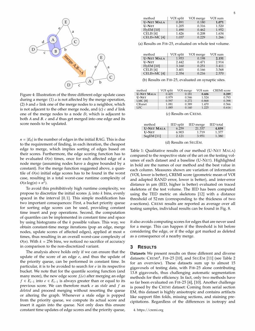
Figure 4: Illustration of the three different edge update casesduring a merge: (1) a is not affected by the merge operation,(2) b and e link one of the merge nodes to a neighbor, whichis not adjacent to the other merge node, and (c) c and d linkone of the merge nodes to a node D, which is adjacent toboth A and B. c and d thus get merged into one edge and itsscore needs to be updated.

n = |E0 | is the number of edges in the initial RAG. This is dueto the requirement of finding, in each iteration, the cheapestedge to merge, which implies sorting of edges based ontheir scores. Furthermore, the edge scoring function has tobe evaluated O(n) times, once for each affected edge of anode merge (assuming nodes have a degree bounded by aconstant). For the merge function suggested above, a quan-tile of O(n) initial edge scores has to be found in the worstcase, resulting in a total worst-case runtime complexity ofO(n log(n) + n2).

To avoid this prohibitively high runtime complexity, wepropose to discretize the initial scores f0 into k bins, evenlyspaced in the interval [0, 1]. This simple modification hastwo important consequences: First, a bucket priority queuefor sorting edge scores can be used, providing constanttime insert and pop operations. Second, the computationof quantiles can be implemented in constant time and spaceby using histograms of the k possible values. This way, weobtain constant-time merge iterations (pop an edge, mergenodes, update scores of affected edges), applied at most ntimes, thus resulting in an overall worst-case complexity ofO(n). With k = 256 bins, we noticed no sacrifice of accuracyin comparison to the non-discretized variant.

The analysis above holds only if we can ensure that theupdate of the score of an edge e, and thus the update ofthe priority queue, can be performed in constant time. Inparticular, it is to be avoided to search for e in its respectivebucket. We note that for the quantile scoring function (andmany more), the new edge score fi(e) after merging an edgef ∈ Ei−1 into e ∈ Ei−1 is always greater than or equal to itsprevious score. We can therefore mark e as stale and f asdeleted and proceed merging without resorting the queueor altering the graph. Whenever a stale edge is poppedfrom the priority queue, we compute its actual score andinsert it again into the queue. Not only does this ensureconstant time updates of edge scores and the priority queue,

method VOI split VOI merge VOI sumU-NET MALA 0.891 0.180 1.071U-NET 1.205 0.316 1.520FlyEM [10] 1.490 0.462 1.952CELIS [4] 1.426 0.208 1.634CELIS+MC [4] 1.037 0.229 1.266

(a) Results on FIB-25, evaluated on whole test volume.

method VOI split VOI merge VOI sumU-NET MALA 1.953 0.198 2.151U-NET 2.442 0.471 2.914FlyEM [10] 3.160 0.251 3.411CELIS [4] 3.401 0.166 3.568CELIS+MC [4] 2.354 0.216 2.570

(b) Results on FIB-25, evaluated on synaptic sites.

method VOI split VOI merge VOI sum CREMI scoreU-NET MALA 0.425 0.181 0.606 0.289U-NET 0.979 0.546 1.524 0.793LMC [8] 0.597 0.272 0.868 0.398CRunet 1.081 0.389 1.470 0.566LFC 1.085 0.140 1.225 0.616

(c) Results on CREMI.

method IED split IED merge IED totalU-NET MALA 6.259 21.337 4.839U-NET 6.903 1.719 1.377SegEM [11] 2.121 3.951 1.380

(d) Results on SEGEM.

Table 1: Qualitative results of our method (U-NET MALA)compared to the respective state of the art on the testing vol-umes of each dataset and a baseline (U-NET). Highlightedin bold are the names of our method and the best value ineach column. Measures shown are variation of information(VOI, lower is better), CREMI score (geometric mean of VOIand adapted RAND error, lower is better), and inter-errordistance in µm (IED, higher is better) evaluated on tracedskeletons of the test volume. The IED has been computedusing the TED metric on skeletons [12] with a distancethreshold of 52 nm (corresponding to the thickness of twoz-sections). CREMI results are reported as average over alltesting samples, individual results can be found in Fig. 8.

it also avoids computing scores for edges that are never usedfor a merge. This can happen if the threshold is hit beforeconsidering the edge, or if the edge got marked as deletedas a consequence of a nearby merge.

3 RESULTS

Datasets We present results on three different and diversedatasets: CREMI4, FIB-25 [10], and SEGEM [11] (see Table 2for an overview). These datasets sum up to almost 15gigavoxels of testing data, with FIB-25 alone contributing13.8 gigavoxels, thus challenging automatic segmentationmethods for their efficiency. In fact, only two methods haveso far been evaluated on FIB-25 [4], [10]. Another challengeis posed by the CREMI dataset: Coming from serial sectionEM, this dataset is highly anisotropic and contains artifactslike support film folds, missing sections, and staining pre-cipitations. Regardless of the differences in isotropy and

4. https://cremi.org

6

300 1500

60 300 600 300

12 60 120 60

12 24 3(84, 268, 268)

(80, 88, 88)

(76, 28, 28)

(72, 8, 8) (68, 4, 4)

(64, 8, 8)

(60, 20, 20)

(56, 56, 56)

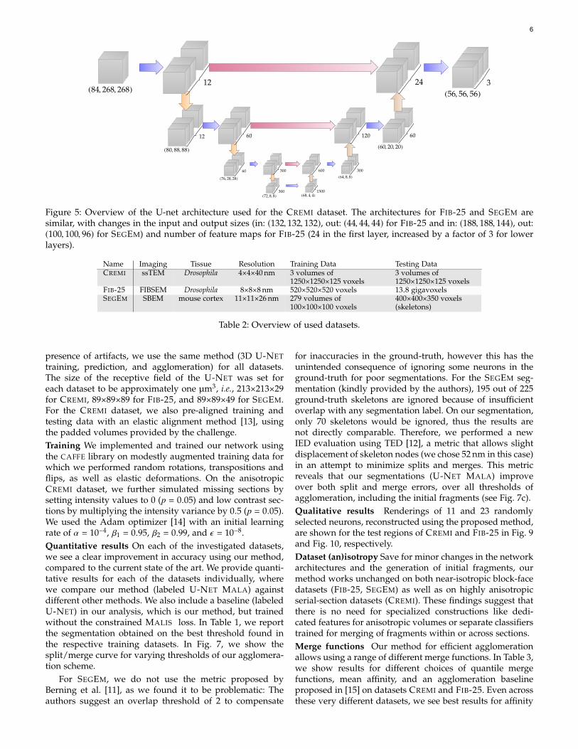
Figure 5: Overview of the U-net architecture used for the CREMI dataset. The architectures for FIB-25 and SEGEM aresimilar, with changes in the input and output sizes (in: (132, 132, 132), out: (44, 44, 44) for FIB-25 and in: (188, 188, 144), out:(100, 100, 96) for SEGEM) and number of feature maps for FIB-25 (24 in the first layer, increased by a factor of 3 for lowerlayers).

Name Imaging Tissue Resolution Training Data Testing DataCREMI ssTEM Drosophila 4×4×40 nm 3 volumes of

1250×1250×125 voxels3 volumes of1250×1250×125 voxels

FIB-25 FIBSEM Drosophila 8×8×8 nm 520×520×520 voxels 13.8 gigavoxelsSEGEM SBEM mouse cortex 11×11×26 nm 279 volumes of

100×100×100 voxels400×400×350 voxels(skeletons)

Table 2: Overview of used datasets.

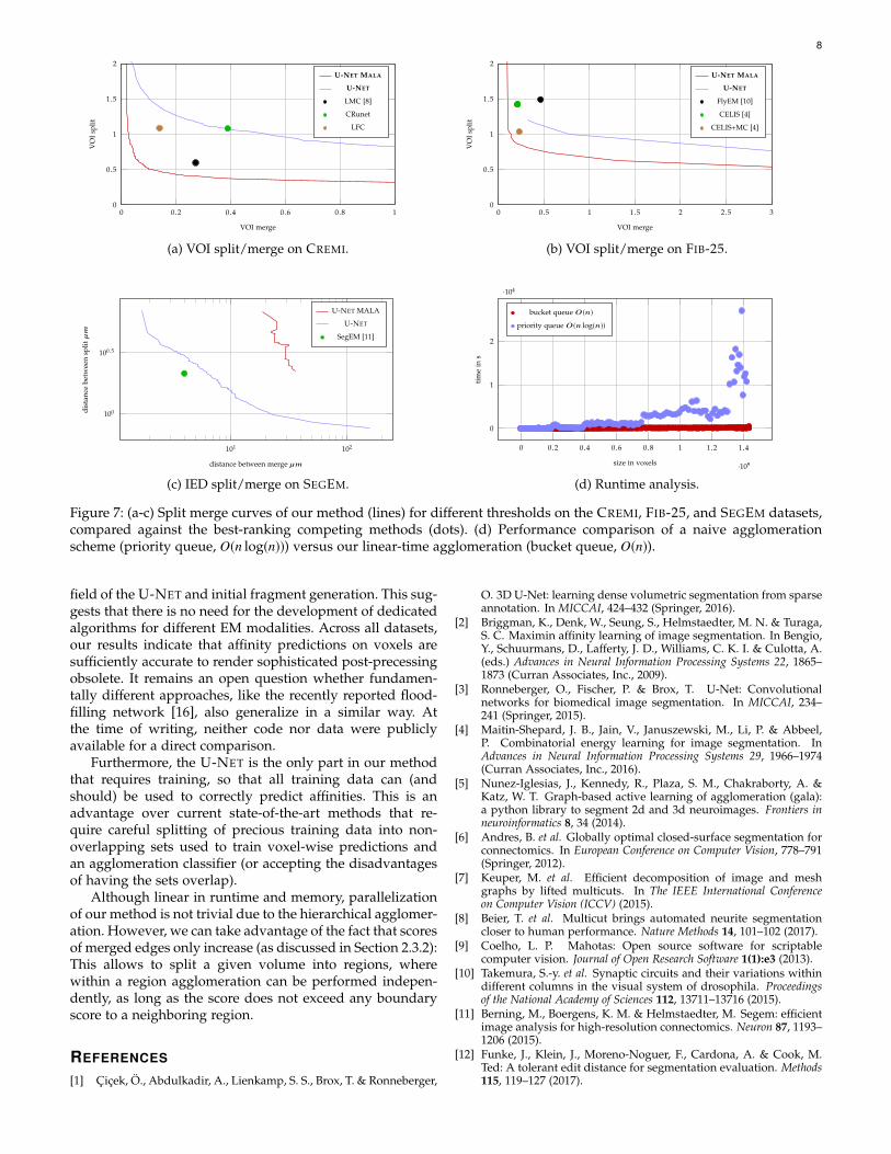
presence of artifacts, we use the same method (3D U-NETtraining, prediction, and agglomeration) for all datasets.The size of the receptive field of the U-NET was set foreach dataset to be approximately one µm3, i.e., 213×213×29for CREMI, 89×89×89 for FIB-25, and 89×89×49 for SEGEM.For the CREMI dataset, we also pre-aligned training andtesting data with an elastic alignment method [13], usingthe padded volumes provided by the challenge.Training We implemented and trained our network usingthe CAFFE library on modestly augmented training data forwhich we performed random rotations, transpositions andflips, as well as elastic deformations. On the anisotropicCREMI dataset, we further simulated missing sections bysetting intensity values to 0 (p = 0.05) and low contrast sec-tions by multiplying the intensity variance by 0.5 (p = 0.05).We used the Adam optimizer [14] with an initial learningrate of α = 10−4, β1 = 0.95, β2 = 0.99, and ε = 10−8.Quantitative results On each of the investigated datasets,we see a clear improvement in accuracy using our method,compared to the current state of the art. We provide quanti-tative results for each of the datasets individually, wherewe compare our method (labeled U-NET MALA) againstdifferent other methods. We also include a baseline (labeledU-NET) in our analysis, which is our method, but trainedwithout the constrained MALIS loss. In Table 1, we reportthe segmentation obtained on the best threshold found inthe respective training datasets. In Fig. 7, we show thesplit/merge curve for varying thresholds of our agglomera-tion scheme.

For SEGEM, we do not use the metric proposed byBerning et al. [11], as we found it to be problematic: Theauthors suggest an overlap threshold of 2 to compensate

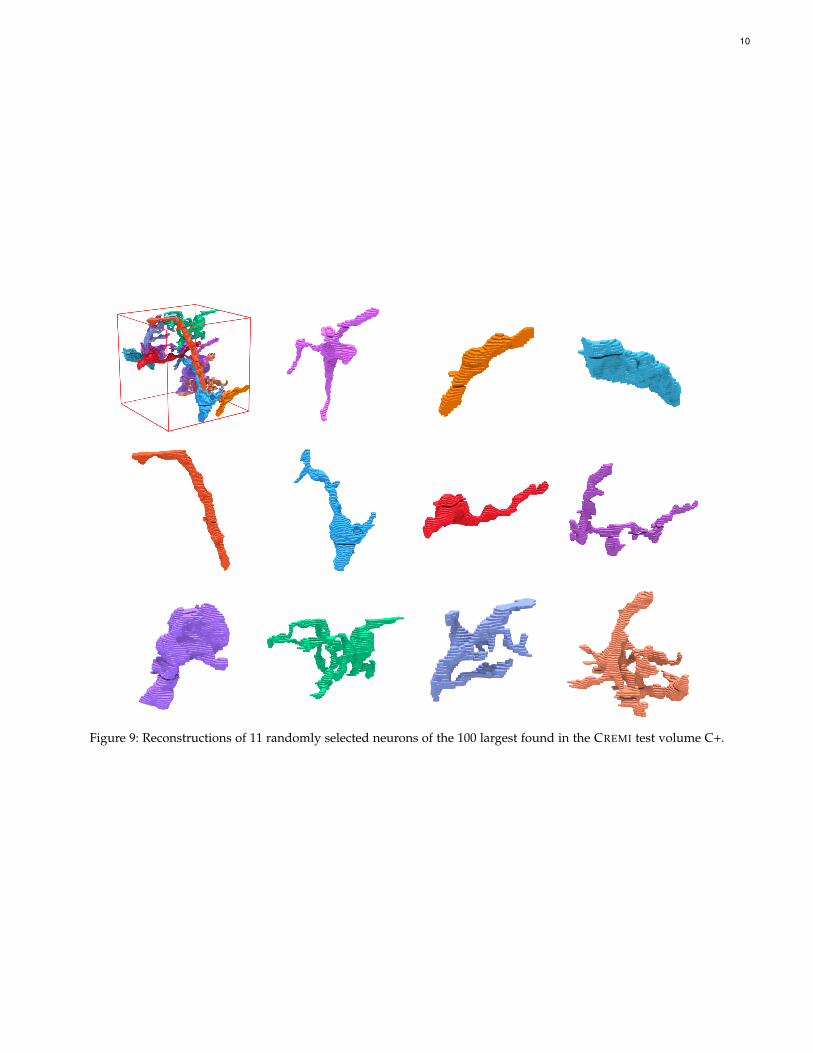
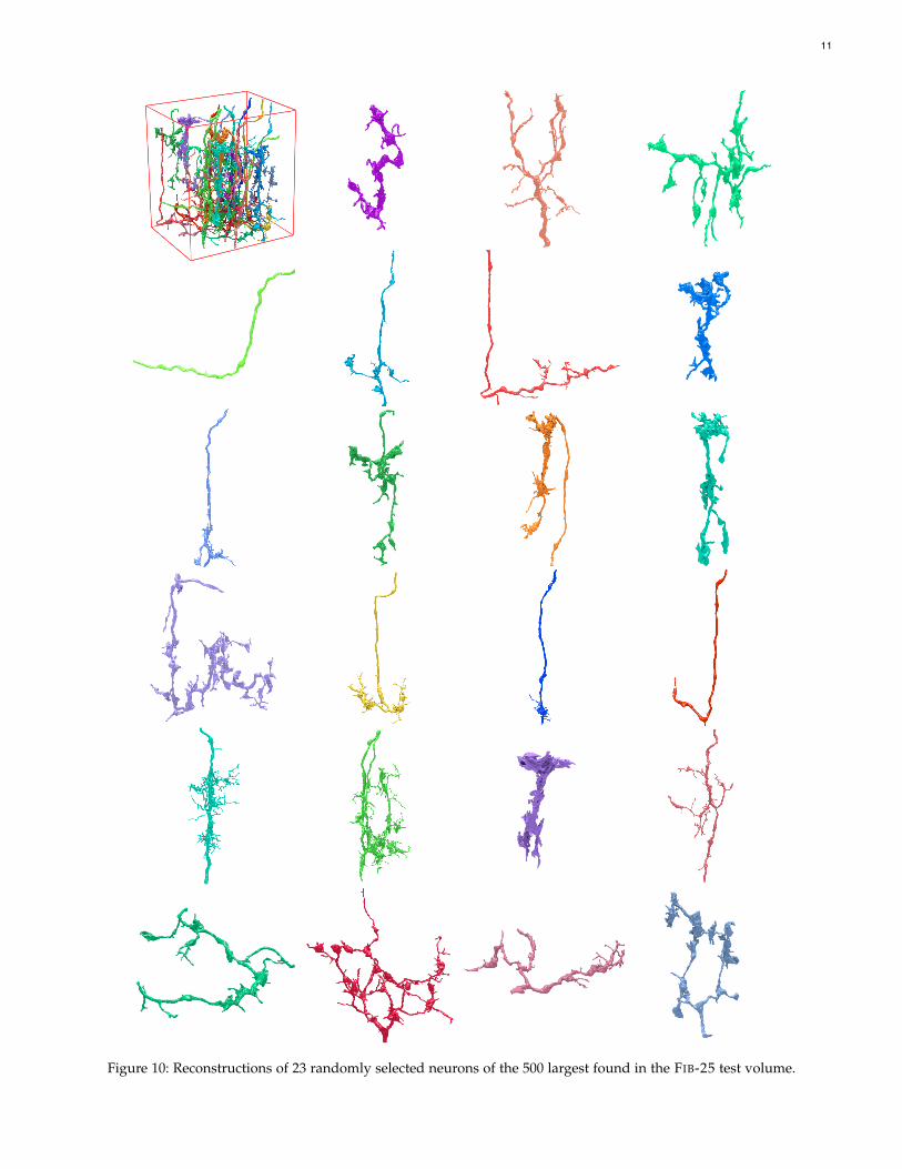
for inaccuracies in the ground-truth, however this has theunintended consequence of ignoring some neurons in theground-truth for poor segmentations. For the SEGEM seg-mentation (kindly provided by the authors), 195 out of 225ground-truth skeletons are ignored because of insufficientoverlap with any segmentation label. On our segmentation,only 70 skeletons would be ignored, thus the results arenot directly comparable. Therefore, we performed a newIED evaluation using TED [12], a metric that allows slightdisplacement of skeleton nodes (we chose 52 nm in this case)in an attempt to minimize splits and merges. This metricreveals that our segmentations (U-NET MALA) improveover both split and merge errors, over all thresholds ofagglomeration, including the initial fragments (see Fig. 7c).Qualitative results Renderings of 11 and 23 randomlyselected neurons, reconstructed using the proposed method,are shown for the test regions of CREMI and FIB-25 in Fig. 9and Fig. 10, respectively.Dataset (an)isotropy Save for minor changes in the networkarchitectures and the generation of initial fragments, ourmethod works unchanged on both near-isotropic block-facedatasets (FIB-25, SEGEM) as well as on highly anisotropicserial-section datasets (CREMI). These findings suggest thatthere is no need for specialized constructions like dedi-cated features for anisotropic volumes or separate classifierstrained for merging of fragments within or across sections.Merge functions Our method for efficient agglomerationallows using a range of different merge functions. In Table 3,we show results for different choices of quantile mergefunctions, mean affinity, and an agglomeration baselineproposed in [15] on datasets CREMI and FIB-25. Even acrossthese very different datasets, we see best results for affinity

7

∗ ∗

w (3, 3, 3)w − 2 (3, 3, 3)

w − 4

max

w

kxw/kx

⊗+

∗w

(kx, ky, kz )w · k

(1, 1, 1)w · k

w w − cx

conv( f1, f2)

pool(kx, ky, kz )

up(kx, ky, kz, f )

crop(cx, cy, cz )

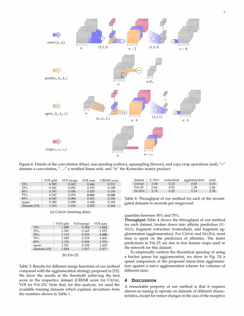
Figure 6: Details of the convolution (blue), max-pooling (yellow), upsampling (brown), and copy-crop operations (red). “∗”denotes a convolution, “ ” a rectified linear unit, and “⊗” the Kronecker matrix product.

VOI split VOI merge VOI sum CREMI score15% 0.583 0.063 0.646 0.21225% 0.441 0.092 0.533 0.18850% 0.397 0.056 0.453 0.15675% 0.347 0.074 0.421 0.14685% 0.347 0.084 0.431 0.156mean 0.380 0.058 0.438 0.149Zlateski [15] 1.015 1.010 2.025 0.364

(a) CREMI (training data).

VOI split VOI merge VOI sum15% 1.480 0.364 1.84425% 1.393 0.163 1.55550% 1.115 0.234 1.35075% 1.085 0.318 1.40285% 1.176 0.394 1.570mean 1.221 0.198 1.418Zlateski [15] 1.054 1.017 2.071

(b) FIB-25.

Table 3: Results for different merge functions of our methodcompared with the agglomeration strategy proposed in [15].We show the results at the threshold achieving the bestscore in the respective dataset (CREMI score for CREMI,VOI for FIB-25). Note that, for this analysis, we used theavailable training datasets which explains deviations fromthe numbers shown in Table 1.

dataset U-NET watershed agglomeration totalCREMI 3.04 0.23 0.83 4.10FIB-25 0.66 0.92 1.28 2.86SEGEM 2.19 0.25 0.14 2.58

Table 4: Throughput of our method for each of the investi-gated datasets in seconds per megavoxel.

quantiles between 50% and 75%.Throughput Table 4 shows the throughput of our methodfor each dataset, broken down into affinity prediction (U-NET), fragment extraction (watershed), and fragment ag-glomeration (agglomeration). For CREMI and SEGEM, mosttime is spent on the prediction of affinities. The fasterpredictions in FIB-25 are due to less feature maps used inthe network for this dataset.

To empirically confirm the theoretical speedup of usinga bucket queue for agglomeration, we show in Fig. 7d aspeed comparison of the proposed linear-time agglomera-tion against a naive agglomeration scheme for volumes ofdifferent sizes.

4 DISCUSSION

A remarkable property of our method is that it requiresalmost no tuning to operate on datasets of different charac-teristics, except for minor changes in the size of the receptive

8

0 0.2 0.4 0.6 0.8 10

0.5

1

1.5

2

VOI merge

VO

Isp

lit

U-NET MALA

U-NET

LMC [8]

CRunet

LFC

(a) VOI split/merge on CREMI.

0 0.5 1 1.5 2 2.5 30

0.5

1

1.5

2

VOI merge

VO

Isp

lit

U-NET MALA

U-NET

FlyEM [10]

CELIS [4]

CELIS+MC [4]

(b) VOI split/merge on FIB-25.

101 102

100

100.5

distance between merge µm

dist

ance

betw

een

splitµm

U-NET MALA

U-NET

SegEM [11]

(c) IED split/merge on SEGEM.

0 0.2 0.4 0.6 0.8 1 1.2 1.4

·109

0

1

2

·104

size in voxels

tim

ein

s

bucket queue O(n)

priority queue O(n log(n))

(d) Runtime analysis.

Figure 7: (a-c) Split merge curves of our method (lines) for different thresholds on the CREMI, FIB-25, and SEGEM datasets,compared against the best-ranking competing methods (dots). (d) Performance comparison of a naive agglomerationscheme (priority queue, O(n log(n))) versus our linear-time agglomeration (bucket queue, O(n)).

field of the U-NET and initial fragment generation. This sug-gests that there is no need for the development of dedicatedalgorithms for different EM modalities. Across all datasets,our results indicate that affinity predictions on voxels aresufficiently accurate to render sophisticated post-precessingobsolete. It remains an open question whether fundamen-tally different approaches, like the recently reported flood-filling network [16], also generalize in a similar way. Atthe time of writing, neither code nor data were publiclyavailable for a direct comparison.

Furthermore, the U-NET is the only part in our methodthat requires training, so that all training data can (andshould) be used to correctly predict affinities. This is anadvantage over current state-of-the-art methods that re-quire careful splitting of precious training data into non-overlapping sets used to train voxel-wise predictions andan agglomeration classifier (or accepting the disadvantagesof having the sets overlap).

Although linear in runtime and memory, parallelizationof our method is not trivial due to the hierarchical agglomer-ation. However, we can take advantage of the fact that scoresof merged edges only increase (as discussed in Section 2.3.2):This allows to split a given volume into regions, wherewithin a region agglomeration can be performed indepen-dently, as long as the score does not exceed any boundaryscore to a neighboring region.

REFERENCES

[1] Cicek, O., Abdulkadir, A., Lienkamp, S. S., Brox, T. & Ronneberger,

O. 3D U-Net: learning dense volumetric segmentation from sparseannotation. In MICCAI, 424–432 (Springer, 2016).

[2] Briggman, K., Denk, W., Seung, S., Helmstaedter, M. N. & Turaga,S. C. Maximin affinity learning of image segmentation. In Bengio,Y., Schuurmans, D., Lafferty, J. D., Williams, C. K. I. & Culotta, A.(eds.) Advances in Neural Information Processing Systems 22, 1865–1873 (Curran Associates, Inc., 2009).

[3] Ronneberger, O., Fischer, P. & Brox, T. U-Net: Convolutionalnetworks for biomedical image segmentation. In MICCAI, 234–241 (Springer, 2015).

[4] Maitin-Shepard, J. B., Jain, V., Januszewski, M., Li, P. & Abbeel,P. Combinatorial energy learning for image segmentation. InAdvances in Neural Information Processing Systems 29, 1966–1974(Curran Associates, Inc., 2016).

[5] Nunez-Iglesias, J., Kennedy, R., Plaza, S. M., Chakraborty, A. &Katz, W. T. Graph-based active learning of agglomeration (gala):a python library to segment 2d and 3d neuroimages. Frontiers inneuroinformatics 8, 34 (2014).

[6] Andres, B. et al. Globally optimal closed-surface segmentation forconnectomics. In European Conference on Computer Vision, 778–791(Springer, 2012).

[7] Keuper, M. et al. Efficient decomposition of image and meshgraphs by lifted multicuts. In The IEEE International Conferenceon Computer Vision (ICCV) (2015).

[8] Beier, T. et al. Multicut brings automated neurite segmentationcloser to human performance. Nature Methods 14, 101–102 (2017).

[9] Coelho, L. P. Mahotas: Open source software for scriptablecomputer vision. Journal of Open Research Software 1(1):e3 (2013).

[10] Takemura, S.-y. et al. Synaptic circuits and their variations withindifferent columns in the visual system of drosophila. Proceedingsof the National Academy of Sciences 112, 13711–13716 (2015).

[11] Berning, M., Boergens, K. M. & Helmstaedter, M. Segem: efficientimage analysis for high-resolution connectomics. Neuron 87, 1193–1206 (2015).

[12] Funke, J., Klein, J., Moreno-Noguer, F., Cardona, A. & Cook, M.Ted: A tolerant edit distance for segmentation evaluation. Methods115, 119–127 (2017).

9

0 0.5 1 1.5 20

0.2

0.4

0.6

0.8

1

VOI split

VO

Im

erge

U-NET MALA

U-NET MALA

U-NET

LMC

CRunet

LFC

00.20.40.60.81

0

0.2

0.4

0.6

0.8

1

RAND split

RA

ND

mer

ge

U-NET MALA

U-NET MALA

U-NET

LMC

CRunet

LFC

U-NET MALA LMC CRunet LFC

0.5

1

1.5

VO

;I

(a) CREMI sample A+

0 0.5 1 1.5 20

0.2

0.4

0.6

0.8

1

VOI split

VO

Im

erge

U-NET MALA

U-NET MALA

U-NET

LMC

CRunet

LFC

00.20.40.60.81

0

0.2

0.4

0.6

0.8

1

RAND split

RA

ND

mer

ge

U-NET MALA

U-NET MALA

U-NET

LMC

CRunet

LFC

U-NET MALA LMC CRunet LFC

0.8

1

1.2

1.4

VO

;I

(b) CREMI sample B+

0 0.5 1 1.5 20

0.2

0.4

0.6

0.8

1

VOI split

VO

Im

erge

U-NET MALA

U-NET MALA

U-NET

LMC

CRunet

LFC

00.20.40.60.81

0

0.2

0.4

0.6

0.8

1

RAND split

RA

ND

mer

ge

U-NET MALA

U-NET MALA

U-NET

LMC

CRunet

LFC

U-NET MALA LMC CRunet LFC

1

1.5

2

VO

;I

(c) CREMI sample C+

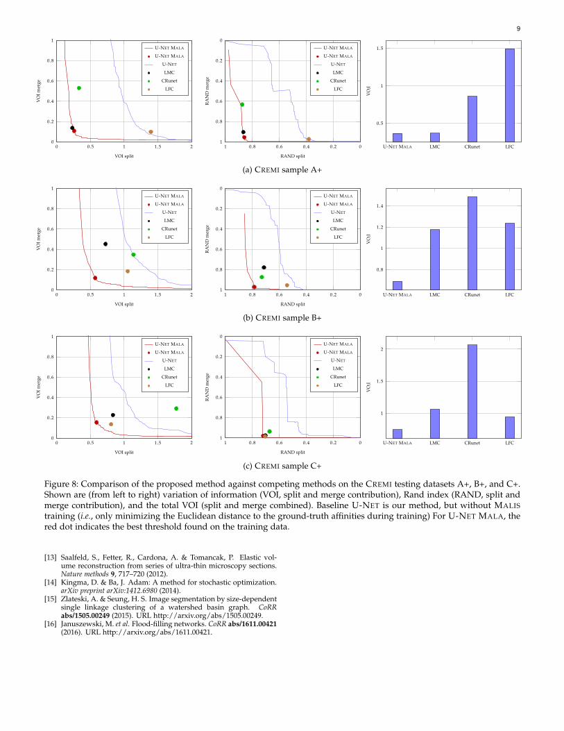
Figure 8: Comparison of the proposed method against competing methods on the CREMI testing datasets A+, B+, and C+.Shown are (from left to right) variation of information (VOI, split and merge contribution), Rand index (RAND, split andmerge contribution), and the total VOI (split and merge combined). Baseline U-NET is our method, but without MALIStraining (i.e., only minimizing the Euclidean distance to the ground-truth affinities during training) For U-NET MALA, thered dot indicates the best threshold found on the training data.

[13] Saalfeld, S., Fetter, R., Cardona, A. & Tomancak, P. Elastic vol-ume reconstruction from series of ultra-thin microscopy sections.Nature methods 9, 717–720 (2012).

[14] Kingma, D. & Ba, J. Adam: A method for stochastic optimization.arXiv preprint arXiv:1412.6980 (2014).

[15] Zlateski, A. & Seung, H. S. Image segmentation by size-dependentsingle linkage clustering of a watershed basin graph. CoRRabs/1505.00249 (2015). URL http://arxiv.org/abs/1505.00249.

[16] Januszewski, M. et al. Flood-filling networks. CoRR abs/1611.00421(2016). URL http://arxiv.org/abs/1611.00421.

10

Figure 9: Reconstructions of 11 randomly selected neurons of the 100 largest found in the CREMI test volume C+.

11

Figure 10: Reconstructions of 23 randomly selected neurons of the 500 largest found in the FIB-25 test volume.