1

7. Multiple Regression IV

ECON 251

Research Methods

2

Functional forms

The logarithmic and exponential functions are two of the most commonly used functions in model formulations.

With the logarithmic and exponential functions we can capture a variety of effects:• marginal effects• diminishing returns• returns to scale• growth rates• odds

3

Properties of logs

Y = A + B ln Y = ln(A + B)

Y = AB ln Y = ln(AB) = ln A + ln B

Y = A/B ln Y = ln(A/B) = ln A - ln B

Y = AB ln Y = ln(AB) = B * ln A

AB e B * ln A

4

Marginal effects and elasticities

What is an elasticity?• % change in Y with respect to a % change in X for a small

change in X

Y

X

X

Y

XXYY

X

Yxy

%

%,

X

Y

Effect Marg

What is a marginal effect?• the change in Y per unit change in X

• example: price elasticity of demand if price increases by 1% quantity demanded changes by ηq,p.

5

Marginal effects and elasticities

Name Functional Form Marginal Effect Elasticity

Linear Y=β0+ β1X β1 β1X/Y

Linear-log Y=β0+ β1lnX β1/X β1/Y

Quadratic Y=β0+ β1X + β2X2 β1 + 2β2X (β1 + 2β2X)X/Y

Log-linear lnY=β0+ β1X β1Y β1X

Double-log lnY=β0+ β1lnX β1Y/X β1

Logistic ln[Y/(1-Y)]=β0+ β1X β1Y(1-Y) β1(1-Y)X

6

Linear-log model Y = β0 + β1 ln X + ε

• used to capture the diminishing marginal returns (product)

X

Y

β0+ β1 ln X

7

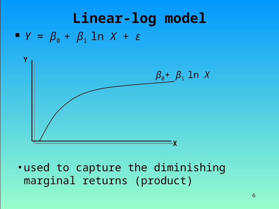
Log-linear (semilog) model

lnY = β0 + β1X + ε

• used to capture constant growth rates• Pt = (1+g)Pt-1 Pt = P0(1+g)t

ln Pt = ln P0 + t ln(1+g) ln Pt = β0 + β1t

where β0 = ln P0 and β1= ln(1+g)

X

Y

eβ0+ β1X

8

Human resource application

theory suggests that the rate of return to an extra year of education is r. Then, for the first period w1 = (1 + r) w0. For, the second period w2 = (1 + r)2 w0, and for s years ws

= (1 + r)s w0. Then, taking logs of both sides yields:

ln(ws) = s ln(1 + r) + ln(w0) = β0 + β1 s

model:• ln(WAGE) = β0 + β1 EDUC + ε

download file: HR.xls

9

Regression StatisticsMultiple R 0.36393R Square 0.1324451Adjusted R Square0.1139865Standard Error 0.2943775Observations 49

ANOVAdf SS MS F Sig F

Regression 1 0.621793 0.62179 7.175245 0.010153Residual 47 4.072933 0.08666Total 48 4.694726

Coefficients S.E. t Stat P-value Lower 95%Upper 95%Intercept 7.1565383 0.119077 60.1 4.18E-46 6.916986 7.396091EDUC 0.0479419 0.017898 2.67866 0.010153 0.011936 0.083947

Human resource application

ln(WAGE) = β0 + β1 EDUC + ε

ln(WAGE)=7.1565+0.0479*EDUC

10

ln(WAGE)= 7.1565 + 0.0479*EDUC

the rate of return to an extra year of education is r ln(1 + r)=0.0479 1 + r = e0.0479 r = 0.0491

Marginal Effect:• say when EDUC = 5:

Y = e7.1565 + 0.0479 * 5 = e7.3962 = 1629.8571• Maginal Effect (X=5) : β1Y = 0.0479*1629.8571=78.14

• How about when EDUC = 6:• Maginal Effect (X=6) : β1Y = 0.0479*1709.8988=81.98

Human resource application – Interpretation

11

So, when a person has 5 year of education, an extra year of education would increase salary by $78.14

when a person has 6 years of education, an extra year of education would increase salary by $81.98

Can you find percentage changes in salaries? % changes:

• when EDUC = 5 78.14/1629.8571=0.04794• when EDUC = 6 81.98/1709.8988=0.04794

so, the interpretation of β1 is the expected % change in Y when X increases by 1.

would a linear model be better (higher adj. R2)?• cannot compare R2 if dependent variable is not the same

Human resource application – Interpretation

12

Log-log (double log) model

popular in estimating demand functions• coefficients are constant elasticities

Example: Demand for bus travel• depends on

―price ―income―price of a substitute good ―other factors

13

Example – Demand for bus travel

Variables (Bus Travel)• BUSTRAVL: demand for urban transportation by bus in

thousands of passenger hours• FARE: bus fare in dollars• GASPRICE: Price of a gallon of gasoline in dollars• INCOME: Average income per capita in dollars• POP: Population in city in thousands• DENSITY: density of population (persons/sq. mile)• LANDAREA: land area of the city (sq. miles)

Find relevant elasticities of demand!

14

Example – Demand for bus travel

Modeling: How does the full model perform? Are there any insignificant variables? Try removing out the most insignificant variable. What

happens? Are there any other insignificant variables? Which variables will you keep for your final model? How does the final model perform? Is there an improvement from the initial to the final model?

15

Regression StatisticsMultiple R 0.7992298R Square 0.6387682Adjusted R Square 0.6086656Standard Error 0.7241214Observations 40

ANOVAdf SS MS F Sig F

Regression 3 33.37971 11.12657 21.21966777 4.3463E-08Residual 36 18.87667 0.524352Total 39 52.25638

Coefficients S.E. t Stat P-value Lower 95% Upper 95%Intercept 45.845675 9.61411 4.768582 3.04076E-05 26.3473557 65.34399INCOME -4.730082 1.021192 -4.631923 4.60006E-05 -6.8011554 -2.659009POP 1.8203709 0.235733 7.722176 3.79544E-09 1.34228245 2.298459LANDAREA -0.970997 0.206807 -4.695192 3.79873E-05 -1.3904208 -0.551574

Example – Demand for bus travel

Final model

What do the coefficients mean?

16

Interpretation: ln(BUSTRAVL) = 45.85 – 4.73 * ln(INCOME)

+1.82 * ln(POP) – 0.97 * ln(LANDAREA) What is income elasticity of demand for bus travel? ηBT,I = -4.73

Is demand for bus travel elastic/inelastic/unit elastic with respect to POPULATION and LANDAREA? (disregard the sign of the coefficient)• if η < 1: inelastic• if η = 1: unit elastic• if η > 1: elastic

Example – Demand for bus travel

17

Example – Demand for bus travel

Question:• Is demand for bus travel elastic with respect to city’s

population? POPULATION

• H0: β2 = 1

• H1: β2 > 1

t0.05,36 = 1.68

t-stat ______________ than the critical value __________ null hypothesis and conclude that demand for bus travel is ___________ w.r.t. population

2

22

bS

bt

18

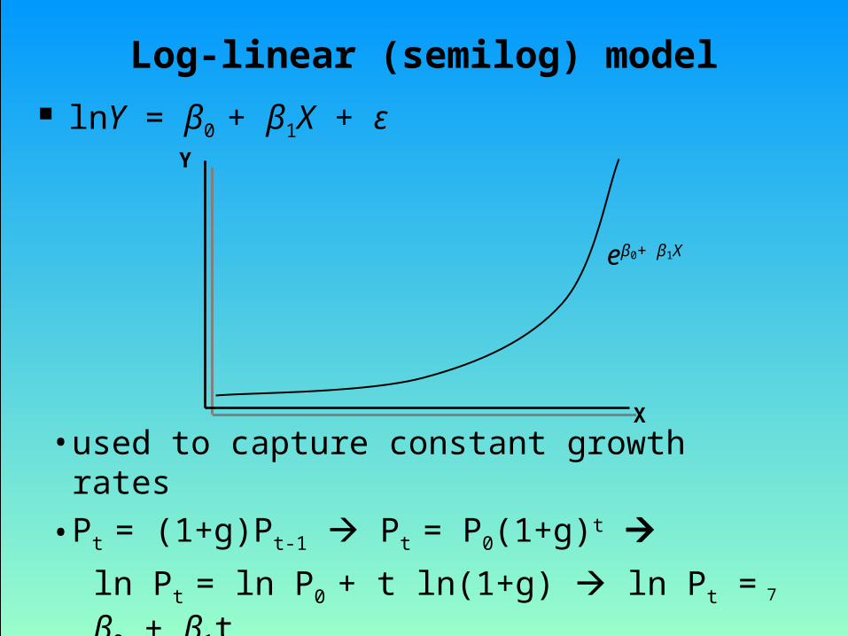
Log-log (double log) model

popular in estimating production functions• Cobb-Douglass production function

used to capture:• elasticities• returns to scale

21),( LAKLKQ

ln Q = ln A + β1 ln K + β2 ln L + ε

19

Cobb-Douglass production function

β1 – elasticity of output wrt capital

β2 – elasticity of output wrt labor

Returns to scale: when you double inputs, what happens to output?

• decreasing RTS: β1 + β2 < 1

• constant RTS: β1 + β2 = 1

• increasing RTS: β1 + β2 > 1

21),( LAKLKQ

20

Example – US manufacturing load the dataset (US manufactring.xls) The data consist of labor hours as the estimate for labor

input (L), total capital expenditures as the estimate for capital input (K), and value added as the estimate for output (Q).

transform the variables into logs run a regression with ln Y being a dependent variable and

ln K and ln L as independent variables what can you say about the elasticities? does the US manufacturing exhibit increasing, constant, or

decreasing returns to scale? write down the US manufacturing production function

21

Example – US manufacturing

Regression StatisticsMultiple R 0.9819243R Square 0.9641754Adj. R Sq. 0.9626827Std Error 0.2667521Observations 51

ANOVAdf SS MS F Sig. F

Regression 2 91.924607 45.962303 645.9310665 1.99686E-35Residual 48 3.4155201 0.0711567Total 50 95.340127

Coeffs S.E. t Stat P-valueIntercept 3.8875995 0.3962283 9.8115137 4.70478E-13lnK 0.5212791 0.0968871 5.3802743 2.18316E-06lnL 0.4683322 0.0989259 4.7341701 1.98088E-05

22

Example – US manufacturing

Interpretation: Elasticities:

• both β1 and β2 < 1 inelastic

Returns to scale• β1 + β2 = 0.5213 + 0.4683 = 0.9896 CRTS

Production functionln Y = 3.8876 + 0.5213 * ln K + 0.4683 * ln Ltake antilogs of both sides:

Y = 48.794 K0.5213 L0.4683