arX

iv:1

807.

0958

2v2

[co

nd-m

at.s

tr-e

l] 5

Dec

201

8

Correlated electronic structure with uncorrelated disorder

A. Ostlin,1 L. Vitos,2, 3, 4 and L. Chioncel5, 1

1Theoretical Physics III, Center for Electronic Correlations and Magnetism,

Institute of Physics, University of Augsburg, D-86135 Augsburg, Germany2Department of Materials Science and Engineering, Applied Materials Physics,

KTH Royal Institute of Technology, SE-10044 Stockholm, Sweden3Department of Physics and Astronomy, Division of Materials Theory,

Uppsala University, Box 516, SE-75120 Uppsala, Sweden4Research Institute for Solid State Physics and Optics,

Wigner Research Center for Physics, P.O. Box 49, H-1525 Budapest, Hungary5Augsburg Center for Innovative Technologies, University of Augsburg, D-86135 Augsburg, Germany

We introduce a computational scheme for calculating the electronic structure of random alloysthat includes electronic correlations within the framework of the combined density functional anddynamical mean-field theory. By making use of the particularly simple parameterization of theelectron Green’s function within the linearized muffin-tin orbitals method, we show that it is possibleto greatly simplify the embedding of the self-energy. This in turn facilitates the implementationof the coherent potential approximation, which is used to model the substitutional disorder. Thecomputational technique is tested on the Cu-Pd binary alloy system, and for disordered Mn-Niinterchange in the half-metallic NiMnSb.

I. INTRODUCTION

Disordered metallic alloys find applications in a largenumber of areas of materials science. Designing alloyswith specific thermal, electrical, and mechanical proper-ties such as conductivity, ductility, and strength, nowa-days commonly starts at the microscopic level1–3. First-principles calculations of the electronic structure offera parameter-free framework to meet specific engineer-ing demands for materials prediction. Advances in theatomistic simulation of physical properties should to alarge extent be attributed to the development of densityfunctional theory (DFT)4,5 within the local density ap-proximation (LDA) or beyond-LDA schemes.

In solids exhibiting disorder the calculation of anyphysical property involves configurational averaging overall realizations of the random variables characterizing thedisorder. In the case of substitutional disorder the sym-metry of the lattice is kept, but the type of atoms in thebasis is randomly distributed. This causes the crystal tolose translational symmetry, making the Bloch theoreminapplicable. Perhaps the most successful approach tosolve the problems associated with substitutional disor-der is the coherent potential approximation6 (CPA). Thepresence of random atomic substitution generates a fluc-tuating external potential which within the CPA is sub-stituted by an effective medium. This effective mediumis energy dependent and is determined self-consistentlythrough the condition that the impurity scattering shouldvanish on average. The CPA is a single-site approxima-tion, which becomes exact in certain limiting cases7. Theexplanation for the good accuracy of the CPA can betraced back to the fact that it becomes exact in the limitof infinite lattice coordination number, Z → ∞8.

The CPA was initially applied to tight-binding Hamil-tonians7, where for binary alloys the CPA equationstake a complex polynomial form that can be solved di-

rectly. Later Gyorffy9 formulated the CPA equations forthe muffin-tin potentials within the multiple-scatteringKorringa-Kohn-Rostocker (KKR) method10,11. Con-sequently, the configurational average could be per-formed over the scattering path operator, instead of theGreen’s function, simplifying the implementation of theCPA for materials calculations12. Later the CPA wasalso implemented within the linearized muffin-tin or-bitals13 (LMTO) basis set14–17. With the advent of thethird-generation exact muffin-tin orbitals18–20 (EMTO)method, and the full-charge density21 (FCD) technique,it was possible to go beyond the atomic-sphere approxi-mation (ASA) with CPA calculations22, and investigatethe energetics of anisotropic lattice distortions. For in-teracting model Hamiltonians, dynamical mean-field the-ory23–25 (DMFT) was also combined with the CPA26–28.Later on the methodology was extended to study real-istic materials containing significant electronic correla-tions within the framework of a combined DFT+DMFTmethod29,30. To treat weak disorder within the frame-work of charge self-consistent LDA+DMFT, the CPA hasbeen implemented within the KKR method31. In an al-ternative approach, the band structures computed fromDFT were mapped to tight-binding model Hamiltonianswere the disorder was treated within the CPA32–35.

In this paper, we introduce a method that can treatsubstitutional disorder effects through the CPA, and elec-tronic correlation effects through DMFT, on an equalfooting for real materials. The method is based on theLDA+DMFT method, zMTO+DMFT, which was re-cently introduced by us36. By making use of the partic-ularly simple parameterized form of the electron Green’sfunction in a linearized basis set, we show that the self-energy can be incorporated naturally within the LMTOformalism as a modification of a single, self-consistentlydetermined parameter. Due to this straightforward in-clusion of the many-body effects, the CPA within the

2

LMTO method retains its general form, and can be usedalmost unaltered for the LDA+DMFT approach.The paper is organized as follows: Section II briefly

reviews the muffin-tin basis sets used in this work. Ashort overview of the LMTO method is given in Sec. II A,with additional formulas given in Appendix A, in order tointroduce the most important quantities needed for theCPA+DMFT implementation. A review of the EMTOmethod, which is the second basis set used in this pa-per, is given in Appendix B. In Sec. III we present themost important development in this paper, a combina-tion of the CPA and the LDA+DMFT method. First, inSec. III A we discuss the principles behind the configura-tion average used for the CPA. Sec. III B shows how theelectronic self-energy can be incorporated into the LMTOpotential functions, while Sec. III C demonstrates howthe potential functions are used as an effective mediumwithin the CPA. The section ends with an outline ofthe full computational scheme. In Sec. IV we presentthe results of the method applied to the binary copper-palladium system, treating the d-electrons of palladiumas correlated. The half-metallic semi-Heusler compoundNiMnSb with disorder is also investigated. Section Vprovides a conclusion of our paper.

II. ELECTRONIC STRUCTURE WITH

MUFFIN-TIN ORBITALS

The standard approach adopted in first-principles elec-tronic structure calculations is the mapping to an ef-fective single-particle equation. The Hohenberg-Kohn-Sham density functional formalism4,5 provides a self-consistent description for the effective one-particle po-tential Veff(r). Within the muffin-tin orbital methods,the effective potential in the Kohn-Sham equations,

[

∇2 − Veff(r)]

Ψj(r) = ǫjΨj(r), (1)

is approximated by spherical potential wells VR(rR)−V0centered on lattice sites R, and a constant interstitialpotential V0, viz.,

Veff(r) ≈ Vmt(rR) ≡ V0 +∑

R

[VR(rR)− V0], (2)

where we introduced the notation rR ≡ rRrR = r − R.We will in the following omit the vector notation forsimplicity. This form of the potential makes it possi-ble to divide the Kohn-Sham equation (1) into radialSchrodinger-like equations within the muffin-tin spheres,and wave equations in the interstitial region, which canbe solved separately. The computational scheme thatwe present in this paper is based on the muffin-tin the-ories developed by Andersen and coworkers, namely theLMTO37–40, and the EMTO18–20,41,42, methods. In thefollowing, we briefly review the main ideas and notationsbehind the LMTO-ASA method.

A. Linear Muffin-Tin Orbitals

The energy-independent linearized muffin-tin orbitalsχαRL(rR), centered at the lattice site R, are given as:

χαRL(rR) = φRL(rR) +

∑

R′L′

φαR′L′(rR)hαRL,R′L′ , (3)

φαRL(rR) = φRL(rR) + φRL(rR)oαRL, (4)

φRL(rR) = φRL(rR)YL(rR). (5)

φRL(rR) is the solution of the radial Schrodinger equationat an arbitrary energy ǫν , usually taken to be the centerof gravity of the occupied part of the band, and oαRL =

〈φRL|φαRL〉 is an overlap integral. L ≡ (l,m) denotes theorbital and azimuthal quantum numbers, respectively.The superscript α denotes the screening representationused in the tight-binding LMTO theory. The expan-sion coefficients hα are determined from the conditionthat the wave function is continuous and differentiableat the sphere boundary at each sphere: hαRL,R′L′(k) =

(cαRL− ǫν)δRR′δLL′ +√

dαRlSαRLR′L′(k)

√

dαR′l′ . Note thatwe are now assuming a translationally invariant latticesystem, so that the Bloch wave vector k is well defined.From now on, R will denote the atoms in the unit cellonly. The coefficient hαRL,R′L′ is parametrized by the

center of the band, cαRL = ǫν − PαRL(ǫν)[P

αRL(ǫν)]

−1, and

the band width parameter dαRL = [PαRL(ǫν)]

−1, both ex-pressed in terms of the potential function Pα

RL and its

energy derivative PαRL evaluated at ǫν . The potential

function Pα and the structure constant Sα are expressedusing the conventional potential function P 0 and the con-ventional structure constant matrix S039:

PαRL = [P 0(1 − αP 0)−1]RL,

SαRLR′L′ = [S0(1− αS0)−1]RLR′L′ . (6)

P 0RL is proportional to the cotangent of the phase shift

created by the potential centered at the sphere at R.Thus, the potential parameters P characterize the scat-tering properties of the atoms placed at the lattice sites.The geometry of the lattice enters through the structureconstants S0, which is independent of the type of atomsoccupying the sites. S0 has a long range behavior in realspace, but is decaying nearly exponentially in the tight-binding β-representation38. The so-called band distor-tion parameter α = (P 0)−1−(Pα)−1 = (S0)−1−(Sα)−1,which is also used to denote the screening representa-tion, gives a relation between the α-representation andthe unscreened representation. In the nearly-orthogonalγ-representation, α = γ, and oγRL = 0, hence the Hamil-tonian Hγ

RLR′L′ is given by:

HγRLR′L′(k) = CRl +

√

∆RlSγRLR′L′(k)

√

∆R′l′ , (7)

where CRl, ∆Rl and γRl are the representation-independent band center-, width- and distortion poten-tial parameters, respectively39,40. The correspondingGreen’s function in the γ-representation is given by:

GγRLR′L′(k, z) = [(z −Hγ(k))]

−1RLR′L′ , (8)

3

where z is an arbitrary complex energy. Further impor-tant relations among the LMTO representations can befound in Appendix A.

III. ELECTRONIC CORRELATIONS AND

DISORDER: THE SINGLE-SITE

APPROXIMATION

In this section we present an LMTO-CPA scheme,that allows to include local self-energies, on the level ofDMFT, for the alloy components. The scheme is imple-mented within the Matsubara representation, and is com-bined with the zMTO+DMFT method36. Section IIIAbriefly discusses the configurational averaging and theCPA, while in Sec. III B we show how DMFT throughthe Dyson equation leads to a renormalization of the pa-rameters of the LMTO-ASA formalism. Section III Ccombines the ideas of the previous two sections, and pro-poses a combined CPA and DMFT loop.

A. Configuration averaging and the CPA

In disordered systems the configurational degrees offreedom characterizing the composition are described bya random variable. Consequently, the potentials at sitesare random in space as in quenched disordered solids. Aparticular realization of the random variable constitutesa configuration of the system in discussion. According toAnderson43 only physically measurable quantities suchas diffusion probabilities, response functions, and densi-ties of states should be configurationally averaged. Asthese quantities are themselves Green’s functions, elec-tronic structure methods using Green’s functions are fa-vored for the study of disordered systems.A major development of the theory of disordered elec-

tronic systems was achieved using the CPA. The CPAbelongs to the class of mean-field theories according towhich the properties of the entire material are determinedfrom the average behavior at a subsystem, usually takento be a single site (cell) in the material. In the mul-tiple scattering description of a disordered system, oneconsiders the propagation of an electron through a disor-dered medium as a succession of elementary scatteringsat the random atomic point scatterers. In the single-siteapproximation one considers only the independent scat-tering off different sites and finally takes the average overall configurations of the disordered system consisting ofthese scatterers. One may then consider any single site ina specific configuration and replace the surrounding ma-terial by a translationally invariant medium, constructedto reflect the ensemble average over all configurations.In the CPA this medium is chosen in a self-consistentway. One assumes that averages over the occupation ofa site embedded in the effective medium yield quantitiesindistinguishable from those associated with a site of themedium itself.

In view of the great progress achieved through the pre-vious implementations of the CPA within muffin-tin or-bitals methods9,12,14–17 we present here in detail a novelcombination of CPA+DMFT in the recently developedzMTO+DMFT method36.

B. Self-energy-modified effective potential

parameters

To deal with the important question concerning theeffect of interaction, we start by observing that withinthe DMFT the self-energy is local and primarily modifiesthe local parameters of the model that describes disor-der. In this section, we show that the presence of a localself-energy, ΣRLRL′(z), modifies the potential function Pentering in the expression of the Green’s function in theLMTO-ASA formalism.We start from the Dyson equation used to construct

the LDA+DMFT Green’s function:

[GDMFTRLR′L′(k, z)]−1 = [GLDA

RLR′L′(k, z)]−1 − ΣRLRL′(z),(9)

where GDMFT/LDARLR′L′ denotes the LDA+DMFT/LDA-level

Green’s function and Σ(z) the self-energy. It is useful todefine an auxiliary Green’s function, the path operatorgαRLR′L′ , as

gαRLR′L′(k, z) = [PαRl(z)− Sα

RLR′L′(k)]−1, (10)

which is valid for a general representation α. In Ap-pendix A we present explicit expressions for the poten-tial functions and auxiliary Green’s functions in differ-ent representations, as well as their connection to thephysical Green’s function. As is apparent in Eq. (10),the full energy- and k-dependence of the path operatoris contained in the potential function and the structureconstants, respectively. Furthermore, the potential func-tion is fully local, i.e., it is diagonal in site index. Inthe following, it will prove convenient to first work in theγ-representation, since here the Green’s function takes aparticularly simple form (see Eq. (A2)):

Gγ,LDARLR′L′(k, z) = ∆

−1/2Rl gγRLR′L′(k, z)∆

−1/2R′l′ , (11)

i.e., it is the path operator normalized by the potentialparameter ∆Rl. Using Eqs. (11) and (A1), the LDAGreen’s function can be evaluated as follows:

[Gγ,LDARLR′L′(k, z)]

−1 = ∆1/2Rl

[

P γ,LDARl (z)− Sγ

RLR′L′(k)]

∆1/2R′l′

= z − CRl −∆1/2Rl S

γRLR′L′(k)∆

1/2R′l′ .

(12)

Hence, the LDA+DMFT Green’s function (9) can bewritten as

[Gγ,DMFTRLR′L′ (k, z)]

−1 =

z − CRl −∆1/2Rl S

γRLR′L′(k)∆

1/2R′l′ − ΣRLRL′(z), (13)

4

i.e., as the resolvent of the Hamiltonian (7) with an em-bedded self-energy. From Eq. (13), it is obvious thatthe same result will follow if the potential parameter CRl

is replaced by an effective parameter, in which the self-energy is embedded, viz.,

CDMFTRLRL′(z) ≡ CRl +ΣRLRL′(z). (14)

Hence the effective potential parameter CDMFTRLRL′ will now

in general be complex, energy-dependent, and have off-diagonal elements. However, CDMFT

RLRL′ is still local. Withthis effective potential parameter, the LDA+DMFT levelGreen’s function can be expressed in a similar form as theLDA-level Green’s function, viz.,

[Gγ,DMFTRLR′L′ (k, z)]

−1 =

∆1/2Rl [P

γ,DMFTRLRL′ (z)− Sγ

RLR′L′(k)]∆1/2R′l′ , (15)

where

P γ,DMFTRLRL′ (z) ≡ P γ,LDA

Rl (z)−∆−1/2Rl ΣRLRL′(z)∆

−1/2R′l′

= ∆−1/2Rl (z − CRl − ΣRLRL′(z))∆

−1/2R′l′

= ∆−1/2Rl (z − CDMFT

RLRL′(z))∆−1/2R′l′ . (16)

Note that due to the self-energy, the effective potentialfunction now has off-diagonal elements.

C. The combined CPA and DMFT loop

For disorder calculations using the CPA, it is more con-venient to use the tight-binding β-representation, since inthis case only the potential functions (and not the struc-ture constants) are random15–17,44 (see also Appendix A).In this case, the representation-dependent potential pa-rameter V β (Eq. (A5)) will be modified accordingly:

V β,DMFTRLRL′ (z) ≡ CRl +ΣRLRL′(z)− ∆Rl

γRl − βl. (17)

For LDA+DMFT calculations, this form of V β,DMFTRLRL′

should be used for the potential function (A4), the path

operator gβ,DMFTRLR′L′ , and the Green’s function (A7), in or-

der for the Dyson equation (9) to be fulfilled. Note thatthe transformations in Eqs. (A6) and (A7) are now nolonger simply scaled as in the LDA case, but are matrixmultiplications due to the presence of off-diagonal termsin the self-energy.In the following, all quantities will be on the dynam-

ical mean-field level, and we suppress the common su-perscript “DMFT” for the coherent medium path oper-ators g, the alloy component path operators gi, the co-herent potential functions P , and the alloy componentpotential functions P i, which will be defined below. Therepresentation-superscript β is kept. An additional su-perscript n appears to represent the iterative nature ofthe equations. The superscript i refers to the index enu-merating the alloy components at a certain site. We also

introduce the concentration of the respective alloy com-ponents i, at a site R, as ciR (0 6 ciR 6 1,

∑

i ciR = 1).

In this paper, the DMFT impurity problem is solvedwithin the imaginary-axis Matsubara frequency repre-sentation, where the Matsubara frequencies are definedas iωξ = (2ξ + 1)iπT , where ξ = 0,±1, ..., and T isthe temperature. In the following, we use the shorthandiω = {iω0, ..., iωξ, ...} to represent the set of all Matsub-ara frequencies. Note that the DMFT impurity problemin principle also can be solved on the real axis, depend-ing on which numerical solver is used. The correspondingCPA equations will also hold for the real energy axis.The CPA self-consistency condition requires that the

sequential substitution by an impurity atom into an effec-tive, translationally-invariant, coherent medium shouldproduce no further electron scattering, on average. InAppendix C we briefly review the CPA+DMFT algo-rithm for the case of a one-band model system. Inthe model Hamiltonian formalism6,7 the ensemble aver-age (coherent) Green’s function (Gc) is constructed fromthe on-site restricted averages of the component Green’sfunction (Gi), according to the formula Gc =

∑

i ciRG

i.A similar formula can be written for muffin-tin potentialsin the multiple scattering formalism, following Gyorffy9,and the averaging of the Green’s function can be trans-fered to the path operator:

gβRLRL′(iω) =∑

i

ciRgi,βRLRL′(iω). (18)

The coherent path operator in the β-representation,

gβRLRL′(iω) =

∫

[P β(iω)− Sβ(k)]−1RLRL′ dk, (19)

has been integrated over the Brillouin zone (BZ). In

Eq. (19), the coherent potential function P β(iω) hasbeen introduced. The alloy component path operatorsin Eq. (18) are found through a Dyson equation,

gi,βRLRL′(iω) = gβRLRL′(iω) +∑

L′′L′′′

gβRLRL′′(iω)

×[

P i,βRL′′RL′′′(iω)− P β

RL′′RL′′′(iω)]

gi,βRL′′′RL′(iω). (20)

Here the potential functions P i,β(iω) are computed ac-cording to Eq. (A4), for each type respectively. In orderto close the CPA equations self-consistently, a new coher-ent potential function has to be determined at each iter-ation. This is done by taking the difference between theinverses of the coherent path operators from the presentiteration n+ 1 and the previous iteration n, as follows:

P β,n+1(iω) = P β,n(iω)− [gβ,n+1(iω)]−1 + [gβ,n(iω)]−1.(21)

The new coherent potential function can be insertedinto Eq. (19), and the cycle can be repeated until self-consistency has been reached. This is performed for eachMatsubara frequency iω. Once self-consistency in the

5

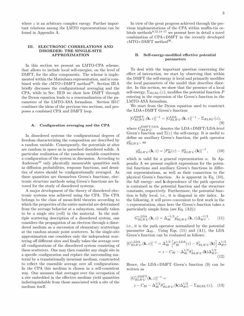
FIG. 1. Schematic flow diagram of the main DMFT-CPA loop, as implemented within the zMTO+DMFT formalism36 . Inputsare the alloy component-dependent potential parameters Ci,∆i and γi, taken from a LDA-level self-consistent EMTO-CPAcalculation. For each Matsubara frequency along the imaginary energy axis, the CPA equations are solved self-consistently.The alloy impurity Green’s functions are supplied to the DMFT impurity problem, which is solved self-consistently, givingalloy component self-energies as output. These self-energies in turn modify the potential parameters which is the key for thecombined self consistency of CPA and DMFT equations. To make the scheme charge self-consistent, the change in the densitydue to correlation, ∆n(r), can be added to the EMTO-CPA charge density n(r), and then the Kohn-Sham equations areiterated until convergence.

CPA equations has been achieved, the Green’s functionsfor each alloy component can be obtained by normalizingthe alloy component path operators in Eq. (20), usingthe transformation in Eq. (A7). These (local) Green’sfunctions are then used as input for the DMFT impurityproblem, with a separate impurity problem for each alloycomponent. For a given interaction strength Umm′m′′m′′′

(defined below) on a particularly chosen alloy compo-nent (i.e. an atomic impurity embedded in the CPA co-herent medium), we solve the interacting problem andalloy component self-energies are produced. The averageover the disorder corresponds in this case to applying theCPA as described above in Eqs. (18)-(21). The coherentself-energy is an implicit quantity, in the self-consistencyloops the alloy component self-energies and the path op-erators are used.

The scheme presented above can easily be incorporatedwithin the formalism of the zMTO+DMFT method36.Here, the EMTO method (see Appendix B for a brief re-view) is employed to solve the Kohn-Sham equations forrandom alloys self-consistently, within the CPA, on thelevel of the LDA. The DMFT impurity problem is thensolved in the Matsubara representation, using lineariza-tion techniques to evaluate the alloy components Green’sfunctions, as presented above. This can be done both onthe LDA-level (setting Σ = 0) and on the DMFT-level(using the self-energy from the DMFT impurity prob-lem). The charge self-consistency is achieved similarlyas in Ref. [36], by computing moments of the alloy com-ponent Green’s function at LDA and DMFT level. Thedifference between the charge densities computed in thisway can then be added as a correction on the LDA-levelcharge computed within the EMTO method. In Fig-

ure 1, we present a schematic picture of the self-consistentloops.

IV. RESULTS

In order to demonstrate the feasibility of our proposedmethod, we apply it to investigate the electronic struc-ture of the binary Cu1−xPdx alloy and the semi-Heuslercompound NiMnSb, with partially exchanged Ni and Mncomponents.

A. Computational details

In all calculations, the kink cancellation condition wasset up for 16 energy points distributed around a semi-circular contour with a diameter of 1 Ry, enclosing thevalence band. The BZ integrations were carried out onan equidistant 13× 13 × 13 k-point mesh in the fcc BZ.For the exchange-correlation potential the local spin den-sity approximation with the Perdew-Wang parameteri-zation45 was used. For the studied alloys a spd-basiswas used. For the Cu-Pd system, the Cu 4s and 3dstates, and for Pd the 5s and 4d states, were treatedas valence. For the case of NiMnSb, the Ni and Mn 4sand 3d states, and for Sb the 5s and 5p states, weretreated as valence. The core electron levels were com-puted within the frozen-core approximation, and weretreated fully-relativistically. The valence electrons weretreated within the scalar-relativistic approximation. Af-ter self-consistency was achieved for NiMnSb, the density

6

of states (DOS) was evaluated with a 21×21×21 k-pointmesh, in order to get an accurate band gap.

To solve the DMFT equations, we used thespin-polarized T -matrix fluctuation-exchange (SPT-FLEX) solver46–50. In this solver, the electron-electron interaction term can be considered in afull spin and orbital rotationally invariant form,

viz. 12

∑

i{m,σ} Umm′m′′m′′′c†imσc†im′σ′cim′′′σ′cim′′σ. Here,

cimσ/c†imσ annihilates/creates an electron with spin σ

on the orbital m at the lattice site i. The Coulombmatrix elements Umm′m′′m′′′ are expressed in the usualway51 in terms of Slater integrals. In moderately corre-lated systems as studied here the modified multi-orbitalfluctuation exchange (FLEX) approximation of Bickersand Scalapino46 proved to be one of the most efficientapproaches47–49,52. The simplifications of the computa-tional procedure in reformulating the FLEX as a DMFTimpurity solver consists in neglecting dynamical inter-actions in the particle-particle channel, considering onlystatic (of T−matrix type) renormalization of the effec-tive interactions. The fluctuating potential Wσ,−σ(iω)is a complex energy-dependent matrix in spin spacewith off-diagonal elementsW σ,−σ(iω) = U m[χσ,−σ(iω)−χσ,−σ0 (iω)]U m, where U m represents the bare vertex ma-

trix corresponding to the transverse magnetic channel,χσ,−σ(iω) is an effective transverse susceptibility ma-

trix, and χσ,−σ0 (iω) is the bare transverse susceptibil-

ity. The fermionic Matsubara frequencies iω were definedabove and m corresponds to the magnetic interactionchannel47,48. In this approximation the electronic self-energy is calculated in terms of the effective interactionsin various channels. The particle-particle contribution tothe self-energy was combined with the Hartree-Fock andthe second-order contributions47,48, which adds to the

the particle-hole contribution Σ(ph)12σ =W σ,σ′

1342(iω)Gσ′

34(iω).The local Green’s functions as well as the electronic self-energies are spin diagonal for collinear magnetic config-urations. Their pole structure, when analytically con-tinued to the real energy axis, produce the appearanceof the peaks located at specific energies determined bythe materials characteristics and the symmetries of theorbitals.

Since specific correlation effects are already includedin the exchange-correlation functional, so-called “doublecounted” terms must be subtracted. To achieve this, wereplace Σσ(E) with Σσ(E) − Σσ(0)

53 in all equations ofthe DMFT procedure29. Physically, this is related tothe fact that DMFT only adds dynamical correlations tothe DFT result54. The Matsubara frequencies were trun-cated after ξ =1024 frequencies, and the temperature wasset to T = 400 K. The values for the average CoulombU and the exchange J parameters are discussed in con-nection with the presentation of the results in each case.The densities of state were computed along a horizontalcontour shifted away from the real energy axis. At theend of the self-consistent calculations, to obtain the self-energy on the horizontal contour, Σ(iω) was analytically

continued by a Pade approximant55,56.

B. Spectral functions and the Fermi surface of

Cu1−xPdx random alloys

We have previously investigated the electronic struc-ture of fcc-Pd58, within the framework of theLDA+DMFT method using the perturbative FLEX im-purity solver59. Recently, the properties of fcc-Pdwere revisited using a lattice (non-local) FLEX solver60.These recent calculations60 support our results using thelocal approximation of the self-energy. Consequently, westudy the electronic correlations in the CuPd alloys usingthe same local DMFT technique as we used before. Inparticular we consider modeling correlations only for thePd alloy component.Discrepancies between the measured photoemission

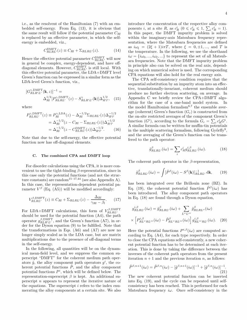
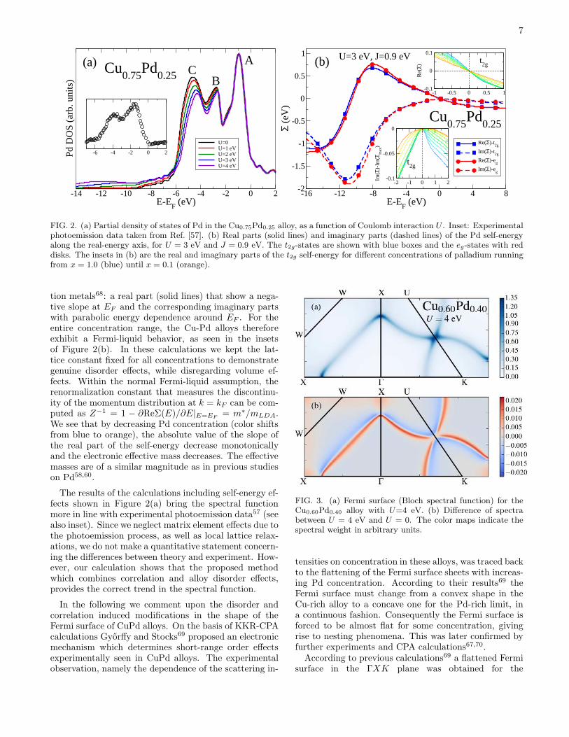
spectra61 and the KKR-CPA spectral functions57,62 forvarious Cu-Pd alloys were often discussed in the litera-ture. In particular LDA-CPA results for the Pd partialDOS of the Cu0.75Pd0.25 alloy reveal a three-peak struc-ture (black line, Figure 2(a), peaks marked by A, B, andC), similar to the DOS of pure fcc-Pd58. Experimentaldata57 on the other hand, see also inset of Figure 2(a),show a contracted band width for the partial DOS and donot resolve the peak at the bottom of the band (markedby C). A detailed discussion concerning these discrepan-cies can be found in Ref. [61]. We note that the frequentlydiscussed reasons for these discrepancies are connected tomatrix element effects63, broadening by electronic self-energy63, and local lattice distortions64–66, that go be-yond the capabilities of standard CPA. Although it isnot our intention to address all of the above inconsis-tencies, our current implementation allows us to addressthe possible source of discrepancy in connection to thecombined disorder and correlation effects.In Figure 2(a) we present the spectral function (DOS)

for the Cu0.75Pd0.25 alloy, as a function of the Coulombparameter U . All curves were evaluated at the latticeconstant given by a linear interpolation between that ofpure Cu and pure Pd (Vegard’s law), which in this casecorresponds to a = 3.68 A. Vegard’s law has previouslybeen shown to hold in a large range of concentrationsfor Cu-Pd within KKR-CPA67. As the Coulomb inter-action is increased, the peak close to the bottom of theband (C) shifts towards the Fermi energy, while the ma-jor peak close to EF (A) remains unchanged. The highbinding energy peak (C) loses intensity with increasingU , and the spectral weight is shifted to higher bindingenergy, where it builds up a satellite structure. A similarbehavior in the spectral weight shift was also found forpure Pd58. In Figure 2(b) we show the Pd self-energiesalong the real-energy axis for the interaction strength ofU = 3 eV and J = 0.9 eV. Note that for different val-ues of these parameters a qualitatively similar behaviorof the self-energy is obtained. This behavior is that ofa typical Fermi-liquid frequently encountered in transi-

7

-14 -12 -10 -8 -6 -4 -2 0 2E-E

F (eV)

Pd D

OS

(arb

. uni

ts)

U=0U=1 eVU=2 eVU=3 eVU=4 eV

-6 -4 -2 0 2

Cu0.75

Pd0.25

A

BC

(a)

-16 -12 -8 -4 0 4 8E-E

F (eV)

-2

-1.5

-1

-0.5

0

0.5

1

Σ (e

V)

Re(Σ)-t2g

Im(Σ)-t2g

Re(Σ)-eg

Im(Σ)-eg

-1 -0.5 0 0.5 1-0.1

0

0.1

Re(

Σ)

-2 -1 0 1 2-0.1

-0.05

0

Im(Σ

)-Im

(Σm

ax)

(b)

Cu0.75

Pd0.25

U=3 eV, J=0.9 eV t2g

t2g

FIG. 2. (a) Partial density of states of Pd in the Cu0.75Pd0.25 alloy, as a function of Coulomb interaction U . Inset: Experimentalphotoemission data taken from Ref. [57]. (b) Real parts (solid lines) and imaginary parts (dashed lines) of the Pd self-energyalong the real-energy axis, for U = 3 eV and J = 0.9 eV. The t2g-states are shown with blue boxes and the eg-states with reddisks. The insets in (b) are the real and imaginary parts of the t2g self-energy for different concentrations of palladium runningfrom x = 1.0 (blue) until x = 0.1 (orange).

tion metals68: a real part (solid lines) that show a nega-tive slope at EF and the corresponding imaginary partswith parabolic energy dependence around EF . For theentire concentration range, the Cu-Pd alloys thereforeexhibit a Fermi-liquid behavior, as seen in the insetsof Figure 2(b). In these calculations we kept the lat-tice constant fixed for all concentrations to demonstrategenuine disorder effects, while disregarding volume ef-fects. Within the normal Fermi-liquid assumption, therenormalization constant that measures the discontinu-ity of the momentum distribution at k = kF can be com-puted as Z−1 = 1 − ∂ReΣ(E)/∂E|E=EF

= m∗/mLDA.We see that by decreasing Pd concentration (color shiftsfrom blue to orange), the absolute value of the slope ofthe real part of the self-energy decrease monotonicallyand the electronic effective mass decreases. The effectivemasses are of a similar magnitude as in previous studieson Pd58,60.

The results of the calculations including self-energy ef-fects shown in Figure 2(a) bring the spectral functionmore in line with experimental photoemission data57 (seealso inset). Since we neglect matrix element effects due tothe photoemission process, as well as local lattice relax-ations, we do not make a quantitative statement concern-ing the differences between theory and experiment. How-ever, our calculation shows that the proposed methodwhich combines correlation and alloy disorder effects,provides the correct trend in the spectral function.

In the following we comment upon the disorder andcorrelation induced modifications in the shape of theFermi surface of CuPd alloys. On the basis of KKR-CPAcalculations Gyorffy and Stocks69 proposed an electronicmechanism which determines short-range order effectsexperimentally seen in CuPd alloys. The experimentalobservation, namely the dependence of the scattering in-

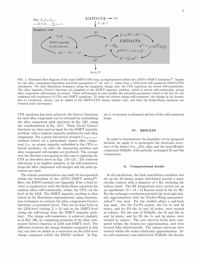
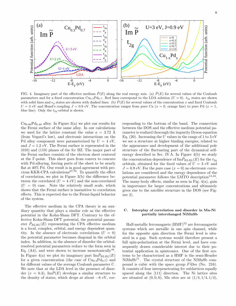
FIG. 3. (a) Fermi surface (Bloch spectral function) for theCu0.60Pd0.40 alloy with U=4 eV. (b) Difference of spectrabetween U = 4 eV and U = 0. The color maps indicate thespectral weight in arbitrary units.

tensities on concentration in these alloys, was traced backto the flattening of the Fermi surface sheets with increas-ing Pd concentration. According to their results69 theFermi surface must change from a convex shape in theCu-rich alloy to a concave one for the Pd-rich limit, ina continuous fashion. Consequently the Fermi surface isforced to be almost flat for some concentration, givingrise to nesting phenomena. This was later confirmed byfurther experiments and CPA calculations67,70.According to previous calculations69 a flattened Fermi

surface in the ΓXK plane was obtained for the

8

-16 -12 -8 -4 0E-E

F (eV)

Pote

ntia

l fun

ctio

n (a

rb. u

nits

) t2g

eg

t2g

eg

t2g

eg

t2g

eg

Cu0.3

Pd0.7

LDA

U=1 eV

U=2 eV

U=3 eV

(a)

Im P~

-16 -12 -8 -4 0E-E

F (eV)

Pote

ntia

l fun

ctio

n (a

rb. u

nits

)

x=0x=0.3x=0.5x=0.7x=1.0

U=3 eV, J=0.9 eVIm P

~

Cu1-x

Pdx

(b)

t2g

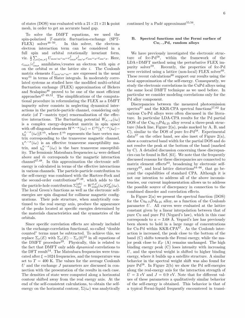
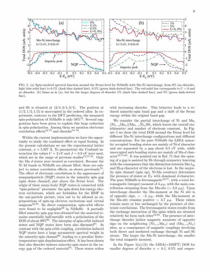
FIG. 4. Imaginary part of the effective medium P (E) along the real energy axis. (a) P (E) for several values of the Coulombparameters and for a fixed concentration Cu0.3Pd0.7. Red lines correspond to the LDA solution (U = 0). t2g states are shown

with solid lines and eg states are shown with dashed lines. (b) P (E) for several values of the concentration x and fixed CoulombU = 3 eV and Hund’s coupling J = 0.9 eV. The concentration ranges from pure Cu (x = 0, orange line) to pure Pd (x = 1,blue line). Only the t2g-orbital is shown.

Cu0.60Pd0.40 alloy. In Figure 3(a) we plot our results forthe Fermi surface of the same alloy. In our calculationswe used for the lattice constant the value a = 3.72 A(from Vegard’s law), and electronic interactions on thePd alloy component were parameterized by U = 4 eV,and J = 1.2 eV. The Fermi surface is represented in the(010) and (110) planes of the fcc BZ. The major part ofthe Fermi surface consists of the electron sheet centeredat the Γ-point. This sheet goes from convex to concavewith Pd-alloying, forcing parts of the sheet to be nearlyflat at 40% Pd. Our result is in good agreement with pre-vious KKR-CPA calculations67,70. To quantify the effectof correlation, we plot in Figure 3(b) the difference be-tween the correlated (U = 4 eV) and the non-correlated(U = 0) case. Note the relatively small scale, whichshows that the Fermi surface is insensitive to correlationeffects. This is expected due to the Fermi-liquid behaviorof the system.

The effective medium in the CPA theory is an aux-iliary quantity that plays a similar role as the effectivepotential in the Kohn-Sham DFT. Contrary to the ef-fective Kohn-Sham DFT potential, the potential param-eter PRLRL(E) representing the CPA effective mediumis a local, complex, orbital, and energy dependent quan-tity. In the absence of electronic correlations (U = 0)the potential parameter becomes diagonal in the orbitalindex. In addition, in the absence of disorder the orbital-resolved potential parameters reduce to the form seen inEq. (A4), and were shown to increase monotonically44.

In Figure 4(a) we plot its imaginary part ImPRLRL(E)for a given concentration (the case of Cu0.3Pd0.7) andfor different values of the average Coulomb parameter U .We note that at the LDA level in the presence of disor-der (x = 0.3), ImP (E) develops a similar structure tothe density of states, which drops at about −8 eV, cor-

responding to the bottom of the band. The connectionbetween the DOS and the effective medium potential pa-rameter is realized thorough the impurity Dyson equationEq. (20). Increasing the U values in the range of 1 to 3 eVwe see a structure at higher binding energies, related tothe appearance and development of the additional polestructure of the fluctuating part of the dynamical self-energy described in Sec. IVA. In Figure 4(b) we study

the concentration dependence of ImPRLRL(E) for the t2gorbitals, obtained for the fixed values of U = 3 eV andJ = 0.9 eV. For the pure case (x = 0) no electronic corre-lations are considered and the energy dependence of thepotential parameter follows the LMTO description13,44.The many-body effects, similar as seen in Fig. 4(a), gainin importance for larger concentrations and ultimatelygives rise to the satellite structure in the DOS (see Fig-ure 2).

C. Interplay of correlation and disorder in Mn-Ni

partially interchanged NiMnSb

Half-metallic ferromagnets (HMF)52 are ferromagneticsystems which are metallic in one spin channel, whilefor the opposite spin direction the Fermi level is situ-ated in a gap. Such systems would therefore present afull spin-polarization at the Fermi level, and have con-sequently drawn considerable interest due to their po-tential application in spintronics. One of the first sys-tems to be characterized as a HMF is the semi-HeuslerNiMnSb71. The crystal structure of the NiMnSb com-pound is cubic with the space group F 43m (No. 216).It consists of four interpenetrating fcc sublattices equallyspaced along the [111] direction. The Ni lattice sitesare situated at (0, 0, 0), Mn sites are at (1/4, 1/4, 1/4),

9

-0.5 -0.4 -0.3 -0.2 -0.1 0 0.1 0.2 0.3 0.4 0.5E-E

F (eV)

-3

-2

-1

0

1

2

3

4

5

Tot

al D

OS

(arb

. uni

ts)

0%0.1%0.5%U=0, 0%

(a)

U=3 eV, J=0.8 eVMn-Ni interchange

NQPImpurity peak

-0.5 -0.4 -0.3 -0.2 -0.1 0 0.1 0.2 0.3 0.4 0.5E-E

F (eV)

-3

-2

-1

0

1

2

3

4

5

Tot

al D

OS

(arb

. uni

ts)

1%5%U=0, 0%

(b)

U=3 eV, J=0.8 eVMn-Ni interchange

NQPImpurity peak

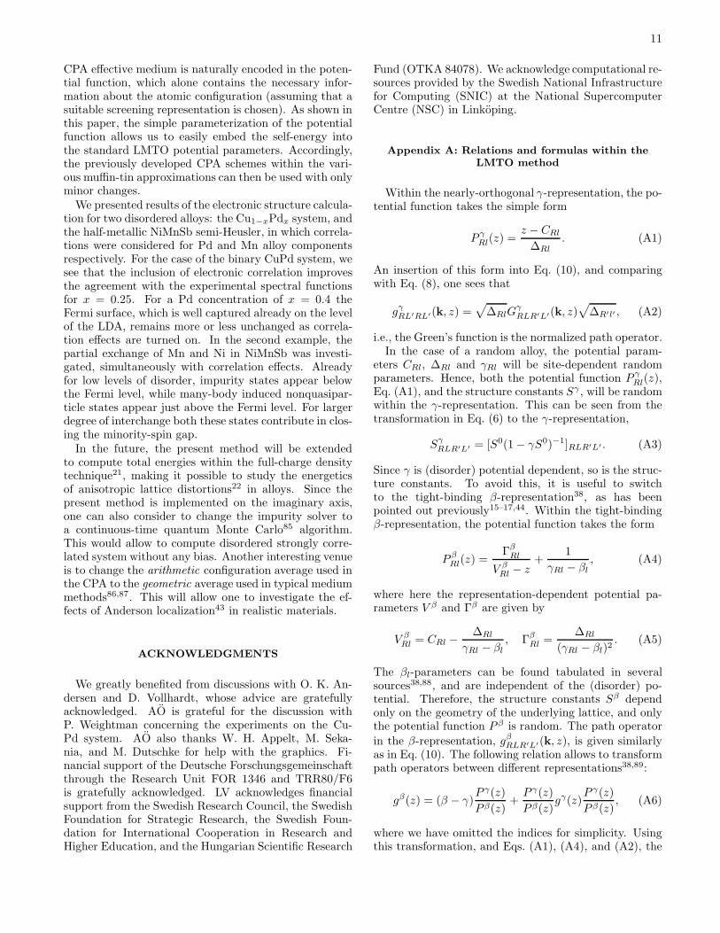
FIG. 5. (a) Spin-resolved spectral function around the Fermi level for NiMnSb with Mn-Ni interchange, from 0% (no disorder,light blue solid line) to 0.1% (dark blue dashed line), 0.5% (green dash-dotted line). The red solid line corresponds to U = 0 andno disorder. (b) Same as in (a), but for the larger degrees of disorder 1% (dark blue dashed line), and 5% (green dash-dottedline).

and Sb is situated at (3/4, 3/4, 3/4). The position at(1/2, 1/2, 1/2) is unoccupied in the ordered alloy. In ex-periment, contrary to the DFT prediction, the measuredspin-polarization of NiMnSb is only 58%72. Several sug-gestions have been given to explain this large reductionin spin-polarization. Among them we mention electroniccorrelation effects52,73 and disorder74–76.

Within the current implementation we have the oppor-tunity to study the combined effect at equal footing. Inthe present calculations we use the experimental latticeconstant, a = 5.927 A. To parametrize the Coulomb in-teraction the values U = 3 eV and J = 0.8 eV were used,which are in the range of previous studies73,77,78. Onlythe Mn d states were treated as correlated. Because theNi 3d bands in NiMnSb are almost filled, these are sub-ject to minor correlation effects, as shown previously78.The effect of electronic correlations is the appearance ofnonquasiparticle (NQP) states in the minority spin gap(spin down channel) just above the Fermi level. Theorigin of these many-body NQP states is connected with“spin-polaron” processes: the spin-down low-energy elec-tron excitations, which are forbidden for the HMF inthe one-particle picture, turn out to be allowed as su-perpositions of spin-up electron excitations and virtualmagnons52,79. By direct computation, spin-orbit effectswere found to be negligible80 in NiMnSb. A partiallyfilled minority spin gap was obtained but the material re-mains essentially half-metallic with a polarization of theDOS of about 99%80. The interplay of spin-orbit inducedstates and NQP states have been also discussed81. Incontrast with the spin-orbit coupling, correlation inducedNQP states have a large asymmetric spectral weight inthe minority-spin channel82, leading to a peculiar finite-temperature spin depolarization effect. It has been shownthat also disorder induces minority-spin states in the en-ergy gap of the ordered material74. These states widen

with increasing disorder. This behavior leads to a re-duced minority-spin band gap and a shift of the Fermienergy within the original band gap.

We consider the partial interchange of Ni and Mn,(Ni1−xMnx)(Mn1−xNix)Sb, which leaves the overall sto-ichiometry and number of electrons constant. In Fig-ure 5 we show the total DOS around the Fermi level fordifferent Mn-Ni interchange configurations and differentconcentrations. For the pure NiMnSb the LSDA minor-ity occupied bonding states are mainly of Ni-d characterand are separated by a gap about 0.5 eV wide, whileunoccupied anti-bonding states are mainly of Mn-d char-acter52,71,83. It was pointed out in Ref. 71 that the open-ing of a gap is assisted by Sb through symmetry loweringwith the consequence that the distinction between Mn-t2gand Sb-p character of the electrons is lost. In the major-ity spin channel (spin up), Ni-Mn covalency determinesthe presence of states at EF with dominant d-character.The pure NiMnSb is ferromagnetic52,71, with a total fer-romagnetic (integer) moment of 4 µB, with the main con-tribution stemming from the Mn-site (∼ 3.8 µB). Uponinterchange disorder the Mn-moment at the Ni site isof opposite sign, ∼ −2 µB, while the Mn-moment atthe Mn-site remains positive ∼ 3.7 µB. These valuesremain more or less unchanged by the presence of elec-tronic correlations. The ferromagnetic states results fromthe exchange interaction of Mn spins which are situatedrelatively far form each other52,84. The presence of inter-change disorder induce magnetic moments of oppositesign on the neighboring (Ni1−xMnx) and (Mn1−xNix)sites, as a consequence of magnetic couplings involvingboth direct and mediated exchange through Ni and Sbatoms. The larger the Mn-Ni interchange, the smallerthe total magnetic moment.

In the Figure 5(a)/(b) the LSDA(+DMFT) DOS forsmaller degrees of disorder x = 0.1, 0.5% and respec-

10

-8 -6 -4 -2 0 2E-E

F (eV)

-3

-2

-1

0

Im(Σ

) (e

V)

Ni-site, downNi-site, upMn-site, downMn-site, upNo disorder, downNo disorder, up

Mn-Σt2g(E)

(a)

U=3 eV, J=0.8 eV

5% disorder

-8 -6 -4 -2 0 2E-E

F (eV)

-3

-2

-1

0

Im(Σ

) (e

V)

-1 0 1

-0.6

-0.4

-0.2

0

0%0.1%0.5%1%5%

Mn-Σe

g(E)

(b)

U=3 eV, J=0.8 eV

5% disorder

FIG. 6. (a) Self-energy along the real axis for the d − t2g states of Mn, at a Mn-Ni interchange disorder of 5%. Dark bluelines correspond to Mn on the Mn-site, red lines correspond to Mn on the Ni-site. Dashed lines with triangles pointing downcorrespond to the spin-down channel, while solid lines with triangles pointing up correspond to the spin-up channel. The Mnself-energy for NiMnSb without disorder (light blue) has been plotted for comparison. (b) Same as in (a), but for the Mn d− egstates. The inset in (b) shows the NQP states in the eg spin-down channel for different disorder concentrations.

tively for larger disorder x = 1%, 5% is seen. The resultsfor the clean, x = 0% (ideal) case, NiMnSb, are pre-sented with red lines (non-interacting, U = 0), and lightblue lines (DMFT). Already at 0.1% disorder (dark bluedashed line) minority states appear below EF . Thesestates are generated by the presence of Ni impurities atthe Mn site, as previously shown by Orgassa et al.74.Furthermore, the upper band edge is shifted to higherenergy. As the disorder is increased, the width of the Niimpurity states are increased. With correlation, minor-ity spin states appear just above the Fermi level. TheseNQP states arise frommany-body electron-magnon inter-actions52. At larger degrees of disorder, see Figure 5(b),the impurity states and the NQP states overlap in energy,removing the spin-down gap. Hence, the combination ofdisorder due to the interchange between Ni and Mn sitesand electronic correlation effects remove the half-metallicgap in NiMnSb.

Figure 6(a)/(b) displays the self-energy along the realenergy axis for the Mn t2g/eg states, respectively, for aMn-Ni interchange of 5%. The dark blue lines correspondto the Mn at the Mn-site, and is similar to the self-energyfor pure NiMnSb (light blue lines). The self-energy be-haves as in previous calculations73, namely: the electronswithin the spin-down channel (blue down-triangles) havea self-energy that is fairly small below EF , but startsto increase above EF . At around 0.5 eV above EF , theself-energy shows a hump, which gives rise to the NQPpeak in the spectral function. The self-energy of spin-up electrons (blue up-triangles) behaves differently, it isrelatively large below EF , while being small in magni-tude above EF . The self-energy for the impurity Mn,situated at the Ni-site, is marked by the red lines in Fig-ure 6(a)/(b). For the spin-down electrons (red down-triangle), the self-energy is large below EF , while it is

small above EF . The trend is opposite for the spin-upchannel electrons (red up-triangle). This opposite behav-ior of the manganese self-energies at different sites reflectsthe anti-parallel configuration of the moments.It is of interest to investigate how the effect of disor-

der, i.e. the degree of Mn-Ni interchange, influence theformation of NQP states. For this reason, in the inset ofFigure 6(b), we plot the Mn-site self-energies of the egorbitals for different disorder concentrations. For minordegrees of Mn-Ni interchange (up to 5%), the suddenincrease in Im Σ(E) just above EF (dashed blue linesof Figure 6), signaling the departure from Fermi liquidbehavior, remains unaffected. It should also be notedthat the Mn self-energy at the Ni-site (Figure 6, redlines), follows the Fermi liquid (quasiparticle) behaviorIm Σ(E) ∝ (E − EF )

2. The Ni d band in NiMnSb is al-most fully occupied, leaving little possibility for magnonsto be excited, therefore weak electron-magnon interactionexists in the Ni-sublattice and no NQP states above EF

are visible in the density of states.

V. CONCLUSION AND OUTLOOK

In this paper we developed a calculation scheme withinthe framework of the density functional theory, whichallows one to study properties of disordered alloys in-cluding electronic correlation effects. We model disorderusing the coherent potential approximation and includelocal but dynamic correlations through dynamical meanfield theory. Similar to our previous implementation36,the DFT-LDA Green’s function is computed directly onthe Matsubara contour. Simultaneously the CPA is im-plemented within the LMTO formalism also in the Mat-subara representation. Within the LMTO formalism the

11

CPA effective medium is naturally encoded in the poten-tial function, which alone contains the necessary infor-mation about the atomic configuration (assuming that asuitable screening representation is chosen). As shown inthis paper, the simple parameterization of the potentialfunction allows us to easily embed the self-energy intothe standard LMTO potential parameters. Accordingly,the previously developed CPA schemes within the vari-ous muffin-tin approximations can then be used with onlyminor changes.We presented results of the electronic structure calcula-

tion for two disordered alloys: the Cu1−xPdx system, andthe half-metallic NiMnSb semi-Heusler, in which correla-tions were considered for Pd and Mn alloy componentsrespectively. For the case of the binary CuPd system, wesee that the inclusion of electronic correlation improvesthe agreement with the experimental spectral functionsfor x = 0.25. For a Pd concentration of x = 0.4 theFermi surface, which is well captured already on the levelof the LDA, remains more or less unchanged as correla-tion effects are turned on. In the second example, thepartial exchange of Mn and Ni in NiMnSb was investi-gated, simultaneously with correlation effects. Alreadyfor low levels of disorder, impurity states appear belowthe Fermi level, while many-body induced nonquasipar-ticle states appear just above the Fermi level. For largerdegree of interchange both these states contribute in clos-ing the minority-spin gap.In the future, the present method will be extended

to compute total energies within the full-charge densitytechnique21, making it possible to study the energeticsof anisotropic lattice distortions22 in alloys. Since thepresent method is implemented on the imaginary axis,one can also consider to change the impurity solver toa continuous-time quantum Monte Carlo85 algorithm.This would allow to compute disordered strongly corre-lated system without any bias. Another interesting venueis to change the arithmetic configuration average used inthe CPA to the geometric average used in typical mediummethods86,87. This will allow one to investigate the ef-fects of Anderson localization43 in realistic materials.

ACKNOWLEDGMENTS

We greatly benefited from discussions with O. K. An-dersen and D. Vollhardt, whose advice are gratefullyacknowledged. AO is grateful for the discussion withP. Weightman concerning the experiments on the Cu-Pd system. AO also thanks W. H. Appelt, M. Seka-nia, and M. Dutschke for help with the graphics. Fi-nancial support of the Deutsche Forschungsgemeinschaftthrough the Research Unit FOR 1346 and TRR80/F6is gratefully acknowledged. LV acknowledges financialsupport from the Swedish Research Council, the SwedishFoundation for Strategic Research, the Swedish Foun-dation for International Cooperation in Research andHigher Education, and the Hungarian Scientific Research

Fund (OTKA 84078). We acknowledge computational re-sources provided by the Swedish National Infrastructurefor Computing (SNIC) at the National SupercomputerCentre (NSC) in Linkoping.

Appendix A: Relations and formulas within the

LMTO method

Within the nearly-orthogonal γ-representation, the po-tential function takes the simple form

P γRl(z) =

z − CRl

∆Rl. (A1)

An insertion of this form into Eq. (10), and comparingwith Eq. (8), one sees that

gγRL′RL′(k, z) =√

∆RlGγRLR′L′(k, z)

√

∆R′l′ , (A2)

i.e., the Green’s function is the normalized path operator.In the case of a random alloy, the potential param-

eters CRl, ∆Rl and γRl will be site-dependent randomparameters. Hence, both the potential function P γ

Rl(z),Eq. (A1), and the structure constants Sγ , will be randomwithin the γ-representation. This can be seen from thetransformation in Eq. (6) to the γ-representation,

SγRLR′L′ = [S0(1− γS0)−1]RLR′L′ . (A3)

Since γ is (disorder) potential dependent, so is the struc-ture constants. To avoid this, it is useful to switchto the tight-binding β-representation38, as has beenpointed out previously15–17,44. Within the tight-bindingβ-representation, the potential function takes the form

P βRl(z) =

ΓβRl

V βRl − z

+1

γRl − βl, (A4)

where here the representation-dependent potential pa-rameters V β and Γβ are given by

V βRl = CRl −

∆Rl

γRl − βl, Γβ

Rl =∆Rl

(γRl − βl)2. (A5)

The βl-parameters can be found tabulated in severalsources38,88, and are independent of the (disorder) po-tential. Therefore, the structure constants Sβ dependonly on the geometry of the underlying lattice, and onlythe potential function P β is random. The path operator

in the β-representation, gβRLR′L′(k, z), is given similarlyas in Eq. (10). The following relation allows to transformpath operators between different representations38,89:

gβ(z) = (β − γ)P γ(z)

P β(z)+P γ(z)

P β(z)gγ(z)

P γ(z)

P β(z), (A6)

where we have omitted the indices for simplicity. Usingthis transformation, and Eqs. (A1), (A4), and (A2), the

12

Green’s function can be obtained from gβRLR′L′(k, z) as88

GγRLR′L′(k, z) =

1

z − V βRl

+

√ΓRl

z − V βRl

gβRLR′L′(k, z)

√ΓR′l′

z − V βR′l′

. (A7)

Note that the transformations in Eqs. (A6) and (A7) aresimply energy-dependent scalings of the path operator,since the potential parameters and the potential func-tions are diagonal matrices.We here briefly mention the accuracy of the presented

expressions. The formulas as written above give correctenergies up to second order in (ǫ− ǫν). A way to improveon this is by a variational procedure90, which produces anew Hamiltonian, giving eigenvalues correct to third or-der. Correspondingly, the substitution z → z+(z−ǫν)3pin Eq. (A7) gives a third-order expression for the po-

tential function39,89. Here, p = 〈φγ |φγ〉 is a (relativelysmall) potential parameter. In order to compare the spec-tra arising from the different orders of LMTO’s, we in-vestigated the DOS for various systems using either sec-ond or third order potential functions, and comparingthe result with the DOS computed from the Hamilto-nian through the spectral representation. We found thatwhile at second order there was no difference between theDOS, for third order there were clear differences betweenthe spectra. This can be attributed to the false polespresent in the third-order potential function90, since theenergy dependence is now not linear, but cubic. In prac-tice, we found that this lead to a loss of spectral weight inthe Green’s function of Eq. (A7), compared to the spec-tral representation. Hence, we in this paper only considersecond order potential functions in Eq. (A7).

Appendix B: Exact Muffin-Tin Orbitals method

One choice of basis for the solution of the Kohn-Shamequation (1) is the energy-dependent exact muffin-tin or-bitals18–20, ψ. They are constructed as a sum of the socalled partial waves, the solutions of the radial equationswithin the spherical muffin-tins, and of the solutions inthe interstitial region. Using this basis, the Kohn-Shameigenfunctions can be expressed as

Ψj(r) =∑

RL

ψaRL(ǫj , rR)v

aRL,j , (B1)

where the superscript a denotes the screening represen-tation used in the EMTO theory18,19.The expansion coefficients, vaRL,j , are determined so

the Ψj(r) is a continuous and differentiable solution ofEq. (1) in all space. This leads to an energy-dependentsecular equation, Ka

RLR′L′(ǫj)vaRL,j = 0, where Ka

RLR′L′

is the so called kink matrix, viz.

KaRLR′L′(k, z) ≡ aδRR′δLL′Da

RL(z)− aSaRLR′L′(k, z).

(B2)

DaRL(z) denotes the EMTO logarithmic derivative

function19,42, and SaRLR′L′(k, z) is the slope matrix41.

The energy dependence of the kink matrix and the sec-ular equation poses no difficulties, since the DFT prob-lem can be solved by Green’s function techniques (see,for example, Ref. 91). By defining the path operatorgaRLR′L′(k, z) as the inverse of the kink matrix,

∑

R′′L′′

KaR′L′R′′L′′(k, z)gaR′′L′′RL(k, z) = δR′RδL′L, (B3)

the poles of the path operator in the complex energyplane will correspond to the eigenvalues of the system.The energy derivative of the kink matrix, KRLR′L′(k, z),gives the overlap matrix for the EMTO basis set41, andhence it can be used to normalize the path operatorgR′′L′′RL(k, z), which gives the EMTO Green’s func-tion19,42

GRLR′L′(k, z) =∑

R′′L′′

gRLR′′L′′(k, z)KR′′L′′R′L′(k, z)

−δRR′δLL′IRL(z), (B4)

where IRL(z) accounts for the unphysical poles of

KRLR′L′(z)19,20. The use of Green’s functions also fa-cilitates the implementation of the CPA, the reader isreferred to Refs. 19, 20, and 22 for more detailed discus-sions.

Appendix C: Illustrative CPA+DMFT algorithm for

model calculations

The algorithm presented in Sec. III C is formulated inthe language of multiple scattering for muffin-tin poten-tials. It represents a generalization of the usual algorithmused for model calculations. In what follows we illustratethe CPA+DMFT self-consistency loop for the one-bandHubbard model with on-site disorder (or the so calledAnderson-Hubbard Hamiltonian):

H = −∑

ijσ

tijc†iσcjσ+U

∑

i

ni↑ni↓+∑

iσ

(ǫi−µσ)niσ (C1)

Here c†iσ(ciσ) create (annihilate) a spin-σ electron on site

i with niσ = c†iσciσ and µσ is the chemical potential ofthe spin-σ electrons. The on-site energies ǫi are chosenas random, while the hopping elements tij are indepen-dent of randomness; thus, short range order is neglected.The coherent and alloy component Green’s functions,and the corresponding self-energies, are complex func-tions of the real energy E. For a multi-band case thesequantities are matrices in orbital space. We start theself-consistency loop with a guess for the self-energy Σc,which includes disorder and correlation effects. We em-phasize that the combined disorder and correlation effectsenter in one single self-energy Σc. The local Green’s func-tion Gc =

∑

k[E + µ− ǫ(k)− Σc]

−1is computed from

the electronic dispersion ǫ(k) (eigenstate of the lattice

13

Hamiltonian in the absence of disorder and electroniccorrelations) and the initial guess for the self-energy Σc.From the coherent (local) Green’s function, alloy com-ponent (i = A,B, . . . ) Green’s functions are computedas

Gi = Gc

[

1− (Vi +ΣDMFTi − Σc)Gc

]−1, (C2)

for a given (fixed) disorder realization. In the nextstep the many-body problem is solved using the DMFTmethodology: the DMFT bath Green’s function is con-structed as: G−1

i = G−1i + ΣDMFT

i . Specific DMFT im-purity solvers produce alloy component many-body self-energies ΣDMFT

i [Gi]. In the next step we request thatthe alloy components should fulfill the CPA equation:Gc =

∑

i ciGi. This corresponds to the averaging overthe disorder realizations. From the newly computed Gc

the coherent self-energy Σc follows directly. To close the

self-consistency loop Gc and Σc are returned into theEq. (C2) to produce new alloy component Green’s func-tions. On a more formal level this algorithm was pre-sented in Ref. 27.

Finally, we mention here the formal equivalence be-tween the equations discussed in the present appendixwith those shown in Sec. III C. The CPA equation Gc =∑

i ciGi and Eq. (18) are equivalent. The local Green’s

function formula (Gc =∑

k[E + µ− ǫ(k)− Σc]

−1) cor-responds to the Eq. (19) in the language of multiple scat-tering. Finally, Eq. (C2) and Eq. (20) are equivalent asthey provide the alloy components computed using theDyson equation. In our recent paper86 we have exten-sively discussed several self-consistent loop algorithmsfor the disorder problem. These include cluster exten-sions and alternative effective medium theories beyondthe CPA.

1 G. B. Olson, Science 288, 993 (2000).2 A. Jain, S. P. Ong, G. Hautier, W. Chen, W. D. Richards,S. Dacek, S. Cholia, D. Gunter, D. Skinner, G. Ceder, andK. A. Persson, APL Materials 1, 011002 (2013).

3 L. Vitos, P. A. Korzhavyi, and B. Johansson,Nature Materials 2, 25 (2002).

4 P. Hohenberg and W. Kohn, Phys. Rev. 136, B864 (1964).5 W. Kohn and L. J. Sham, Phys. Rev. 140, A1133 (1965).6 P. Soven, Phys. Rev. 156, 809 (1967).7 B. Velicky, S. Kirkpatrick, and H. Ehrenreich,Phys. Rev. 175, 747 (1968).

8 R. Vlaming and D. Vollhardt,Phys. Rev. B 45, 4637 (1992).

9 B. L. Gyorffy, Phys. Rev. B 5, 2382 (1972).10 J. Korringa, Physica 13, 392 (1947).11 W. Kohn and N. Rostoker, Physical Review 94, 1111

(1954).12 G. M. Stocks, R. W. Willams, and J. S. Faulkner,

Phys. Rev. B 4, 4390 (1971).13 O. K. Andersen, Phys. Rev. B 12, 3060 (1975).14 J. Kudrnovsky, V. Drchal, and J. Masek,

Phys. Rev. B 35, 2487 (1987).15 J. Kudrnovsky and V. Drchal,

Phys. Rev. B 41, 7515 (1990).16 I. Abrikosov, Y. Vekilov, and A. Ruban,

Physics Letters A 154, 407412 (1991).17 I. A. Abrikosov and H. L. Skriver,

Phys. Rev. B 47, 16532 (1993).18 O. K. Andersen, O. Jepsen, and G. Krier, Lectures on

Methods of Electronic Structure Calculation (World Scien-tific, Singapore, 1994).

19 L. Vitos, Phys. Rev. B 64, 014107 (2001).20 L. Vitos, Computational Quantum Mechanics for Materials

Engineers (Springer, London, 2010).21 L. Vitos, J. Kollar, and H. L. Skriver,

Phys. Rev. B 49, 16694 (1994).22 L. Vitos, I. A. Abrikosov, and B. Johansson,

Phys. Rev. Lett. 87, 156401 (2001).23 W. Metzner and D. Vollhardt, Phys. Rev. Lett. 62, 324

(1989).

24 A. Georges, G. Kotliar, W. Krauth, and M. J. Rozenberg,Rev. Mod. Phys. 68, 13 (1996).

25 G. Kotliar and D. Vollhardt, Physics Today 57, 53 (2004).26 V. Janis and D. Vollhardt, Phys. Rev. B 46, 15712 (1992).27 M. Ulmke, V. Janis, and D. Vollhardt, Phys. Rev. B 51,

10411 (1995).28 Y. Kakehashi, Phys. Rev. B 66, 104428 (2002).29 G. Kotliar, S. Y. Savrasov, K. Haule, V. S. Oudovenko,

O. Parcollet, and C. A. Marianetti, Rev. Mod. Phys. 78,865 (2006).

30 K. Held, Adv. Phys. 56, 829 (2007).31 J. Minar, L. Chioncel, A. Perlov, H. Ebert, M. I. Kat-

snelson, and A. I. Lichtenstein, Phys. Rev. B 72, 045125(2005).

32 P. Wissgott, A. Toschi, G. Sangiovanni, and K. Held,Phys. Rev. B 84, 085129 (2011).

33 M. A. Korotin, Z. V. Pchelkina, N. A. Sko-rikov, E. Z. Kurmaev, and V. I. Anisimov,Journal of Physics: Condensed Matter 26, 115501 (2014).

34 A. S. Belozerov, A. I. Poteryaev, S. L.Skornyakov, and V. I. Anisimov,Journal of Physics: Condensed Matter 27, 465601 (2015).

35 A. S. Belozerov and V. I. Anisimov,Journal of Physics: Condensed Matter 28, 345601 (2016).

36 A. Ostlin, L. Vitos, and L. Chioncel,Phys. Rev. B 96, 125156 (2017).

37 O. K. Andersen, Phys. Rev. B 2, 883 (1970).38 O. K. Andersen and O. Jepsen, Phys. Rev. Lett. 53, 2571

(1984).39 O. K. Andersen, O. Jepsen, and M. Sob, Electronic Band

Structure and Its Applications (Springer Verlag, Berlin,1986).

40 H. L. Skriver, The LMTO Method (Springer, Berlin, 1984).41 O. K. Andersen and T. Saha-Dasgupta, Phys. Rev. B 62,

R16219 (2000).42 L. Vitos, H. L. Skriver, B. Johansson, and J. Kollar,

Comp. Mat. Sci. 18, 24 (2000).43 P. W. Anderson, Phys. Rev. 109, 1492 (1958).44 O. Gunnarsson, O. Jepsen, and O. K. Andersen,

Phys. Rev. B 27, 7144 (1983).

14

45 J. P. Perdew and Y. Wang, Phys. Rev. B 45, 13244 (1992).46 N. E. Bickers and D. J. Scalapino, Ann. Phys. (N. Y.) 193,

206 (1989).47 A. I. Lichtenstein and M. I. Katsnelson, Phys. Rev. B 57,

6884 (1998).48 M. I. Katsnelson and A. I. Lichtenstein, J. Phys.: Condens.

Matter 11, 1037 (1999).49 L. V. Pourovskii, M. I. Katsnelson, and A. I. Lichtenstein,

Phys. Rev. B 72, 115106 (2005).50 O. Granas, I. D. Marco, P. Thunstrom, L. Nord-

strom, O. Eriksson, T. Bjorkman, and J. Wills,Computational Materials Science 55, 295302 (2012).

51 M. Imada, A. Fujimori, and Y. Tokura, Rev. Mod. Phys.70, 1039 (1998).

52 M. I. Katsnelson, V. Y. Irkhin, L. Chioncel, A. I. Licht-enstein, and R. A. de Groot, Rev. Mod. Phys. 80, 315(2008).

53 A. I. Lichtenstein, M. I. Katsnelson, and G. Kotliar, Phys.Rev. Lett. 87, 067205 (2001).

54 A. G. Petukhov, I. I. Mazin, L. Chioncel, and A. I. Licht-enstein, Phys. Rev. B 67, 153106 (2003).

55 H. J. Vidberg and J. W. Serene, J. Low Temp. Phys. 29,179 (1977).

56 A. Ostlin, L. Chioncel, and L. Vitos,Phys. Rev. B 86, 235107 (2012).

57 H. Wright, P. Weightman, P. T. Andrews, W. Folkerts,C. F. J. Flipse, G. A. Sawatzky, D. Norman, and H. Pad-more, Phys. Rev. B 35, 519 (1987).

58 A. Ostlin, W. H. Appelt, I. Di Marco, W. Sun,M. Radonjic, M. Sekania, L. Vitos, O. Tjernberg, andL. Chioncel, Phys. Rev. B 93, 155152 (2016).

59 M. I. Katsnelson and A. I. Lichtenstein, Eur. Phys. J. B30, 9 (2002).

60 S. Y. Savrasov, G. Resta, and X. Wan,Phys. Rev. B 97, 155128 (2018).

61 P. Weightman and R. Cole,J. Electron. Spectrosc. Relat. Phenom. 178-179, 100111 (2010).

62 H. Winter, P. J. Durham, W. M. Temmerman, and G. M.Stocks, Phys. Rev. B 33, 2370 (1986).

63 T.-U. Nahm, M. Han, S.-J. Oh, J.-H. Park, J. W. Allen,and S.-M. Chung, Phys. Rev. Lett. 70, 3663 (1993).

64 P. Weightman, H. Wright, S. D. Waddington, D. van derMarel, G. A. Sawatzky, G. P. Diakun, and D. Norman,Phys. Rev. B 36, 9098 (1987).

65 J. M. C. Thornton, P. Unsworth, M. A. Newell, P. Weight-man, C. Jones, R. Bilsborrow, and D. Norman,EPL (Europhysics Letters) 26, 259 (1994).

66 Y. Kucherenko, A. Y. Perlov, A. N. Yaresko,V. N. Antonov, and P. Weightman,Phys. Rev. B 57, 3844 (1998).

67 I. Wilkinson, R. J. Hughes, Z. Major, S. B. Dugdale,M. A. Alam, E. Bruno, B. Ginatempo, and E. S. Giu-liano, Phys. Rev. Lett. 87, 216401 (2001).

68 A. Grechnev, I. Di Marco, M. I. Katsnelson, A. I. Lichten-stein, J. Wills, and O. Eriksson, Phys. Rev. B 76, 035107(2007).

69 B. L. Gyorffy and G. M. Stocks,Phys. Rev. Lett. 50, 374 (1983).

70 E. Bruno, B. Ginatempo, and E. S. Giuliano,Phys. Rev. B 63, 174107 (2001).

71 R. A. de Groot, F. M. Mueller, P. G. van Engen, andK. H. J. Buschow, Phys. Rev. Lett. 50, 2024 (1983).

72 R. J. Soulen, J. M. Byers, M. S. Osofsky, B. Nadgorny,T. Ambrose, S. F. Cheng, P. R. Broussard, C. Tanaka,J. Nowak, J. S. Moodera, A. Barry, and J. M. D. Coey,Science 282, 85 (1998).

73 L. Chioncel, M. I. Katsnelson, R. A. de Groot, and A. I.Lichtenstein, Phys. Rev. B 68, 144425 (2003).

74 D. Orgassa, H. Fujiwara, T. C. Schulthess, and W. H.Butler, Phys. Rev. B 60, 13237 (1999).

75 J. J. Attema, C. M. Fang, L. Chioncel, G. A. de Wijs,A. I. Lichtenstein, and R. A. de Groot, J. Phys.: Condens.Matter 16, S5517 (2004).

76 M. Ekholm, P. Larsson, B. Alling,U. Helmersson, and I. A. Abrikosov,Journal of Applied Physics 108, 093712 (2010).

77 H. Allmaier, L. Chioncel, E. Arrigoni, M. I. Katsnelson,and A. I. Lichtenstein, Phys. Rev. B 81, 054422 (2010).

78 C. Morari, W. H. Appelt, A. Ostlin, A. Prinz-Zwick,U. Schwingenschlogl, U. Eckern, and L. Chioncel,Phys. Rev. B 96, 205137 (2017).

79 D. M. Edwards and J. A. Hertz, Journal of Physics F-MetalPhysics 3, 2191 (1973).

80 P. Mavropoulos, K. Sato, R. Zeller, P. H. Dederichs,V. Popescu, and H. Ebert, Phys. Rev. B 69, 054424(2004).

81 L. Chioncel, E. Arrigoni, M. I. Katsnelson, and A. I. Licht-enstein, Phys. Rev. Lett. 96, 137203 (2006).

82 L. Chioncel, Y. Sakuraba, E. Arrigoni, M. I. Katsnelson,M. Oogane, Y. Ando, T. Miyazaki, E. Burzo, and A. I.Lichtenstein, Phys. Rev. Lett. 100, 086402 (2008).

83 A. Yamasaki, L. Chioncel, A. I. Lichtenstein, and O. K.Andersen, Phys. Rev. B 74, 024419 (2006).

84 E. Sasioglu, L. M. Sandratskii, and P. Bruno, J. Phys.:Condens. Matter 17, 995 (2005).

85 E. Gull, A. J. Millis, A. I. Lichtenstein,A. N. Rubtsov, M. Troyer, and P. Werner,Rev. Mod. Phys. 83, 349 (2011).

86 H. Terletska, Y. Zhang, L. Chioncel, D. Vollhardt, andM. Jarrell, Phys. Rev. B 95, 134204 (2017).

87 H. Terletska, Y. Zhang, K.-M. Tam, T. Berlijn,L. Chioncel, N. S. Vidhyadhiraja, and M. Jarrell,Applied Sciences 8 (2018), 10.3390/app8122401.

88 H. L. Skriver and N. M. Rosengaard,Phys. Rev. B 43, 9538 (1991).

89 O. K. Andersen, Z. Pawlowska, and O. Jepsen,Phys. Rev. B 34, 5253 (1986).

90 O. K. Andersen, T. Saha-Dasgupta, R. W. Tank, C. Ar-cangeli, O. Jepsen, and G. Krier, in Electronic Structure

and Physical Properties of Solids, edited by H. Dreysse(Springer Verlag, Berlin Heidelberg, 1999) pp. 3–84.

91 R. Zeller, J. Deutz, and P. Dederichs,Solid State Communications 44, 993997 (1982).