1 © 2006 by Nelson, a division of Thomson Canada Limited Slides developed by: William Rentz & Al Kahl University of Ottawa Web Chapter 19 Decisions Under

1© 2006 by Nelson, a division of Thomson Canada Limited

Slides developed by:

William Rentz& Al Kahl

University of Ottawa

Web Chapter 19

Decisions Under Risk and Uncertainty


• Methods of Comparing Different Risks

• Decision Making Under Uncertainty

• Managing Risk and Uncertainty

Topics


• Very few business decisions involve certainty in which an action invariably leads to a specific outcome.

• Most decisions involve a gamble, where the probabilities can be known or unknown and outcomes can be known or unknown

• Risk – exits whenever all the possible outcomes and the probabilities on these outcomes are known» e.g., Roulette Wheel or Dice

• Uncertainty – exits whenever the possible outcomes or the probabilities are unknown» e.g., Drilling for oil in an unknown field

• Unknowingness – when each action has unknown consequences so that the outcomes can NOT be determined.» e.g., the chance and impact of a worldwide nuclear war

Overview


Subjective and Informal Decision Approach

(1)

• Often, probabilities and outcomes are NOT precisely measurable. They are more subjective.

• Managers who must select between two mutually exclusive projects of about the same net returns will tend to pick the one that "feels" less risky.


• When one investment has substantially higher expected return and higher risk, decision makers must subjectively determine if the additional risk is offset sufficiently by the higher return.» These trade-offs can be seen in two continuous probability

distributions for risky project B and less risky project A.

Subjective and Informal Decision Approach

(2)


Continuous Probability Distributions

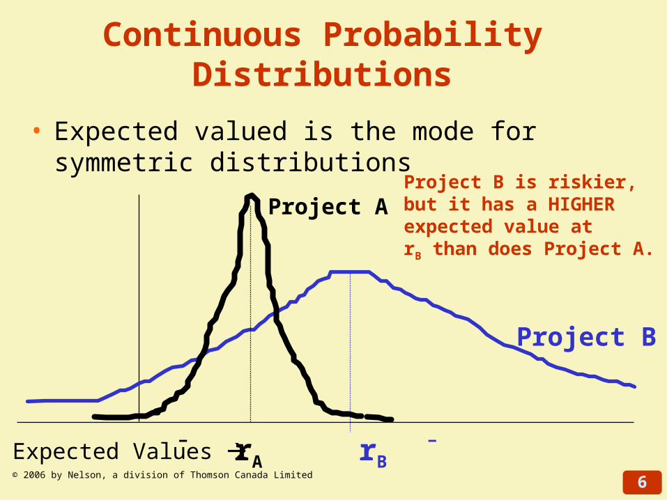
• Expected valued is the mode for symmetric distributions

rBrA

Project B

Project AProject B is riskier, but it has a HIGHER expected value atrB than does Project A.

Expected Values - -


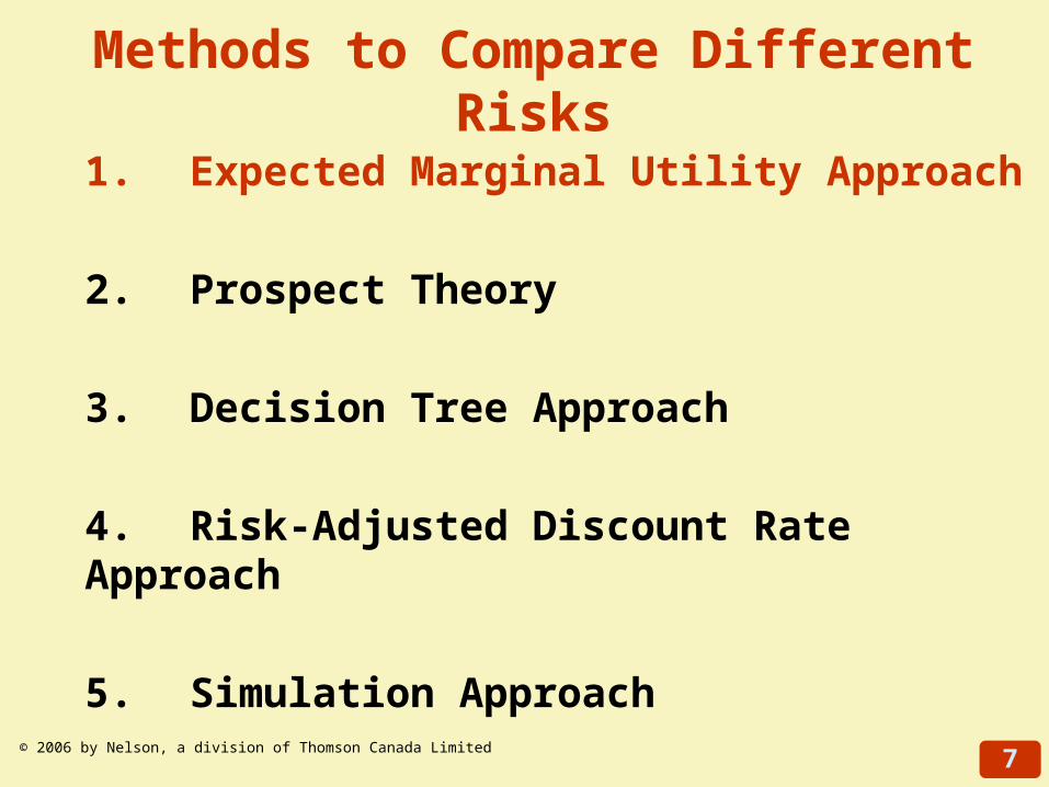
Methods to Compare Different Risks

1. Expected Marginal Utility Approach

2. Prospect Theory

3. Decision Tree Approach

4. Risk-Adjusted Discount Rate Approach

5. Simulation Approach


1. Expected Marginal Utility Approach

• Dollar payoffs do NOT always measure the pain or joy of outcomes

• An example of how people seem NOT to use purely the money payoffs is the St. Petersburg Paradox.


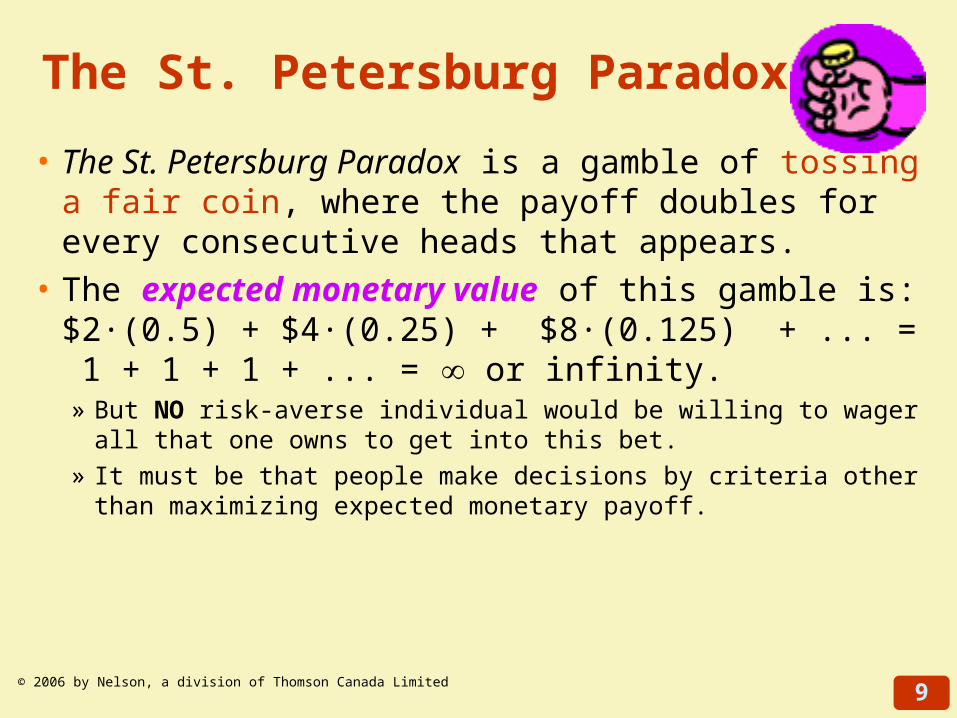
The St. Petersburg Paradox

• The St. Petersburg Paradox is a gamble of tossing a fair coin, where the payoff doubles for every consecutive heads that appears.

• The expected monetary value of this gamble is: $2·(0.5) + $4·(0.25) + $8·(0.125) + ... = 1 + 1 + 1 + ... = or infinity.» But NO risk-averse individual would be willing to wager all that one

owns to get into this bet. » It must be that people make decisions by criteria other than

maximizing expected monetary payoff.


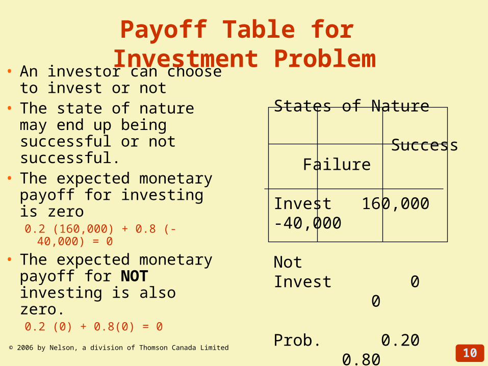
• An investor can choose to invest or not

• The state of nature may end up being successful or not successful.

• The expected monetary payoff for investing is zero 0.2 (160,000) + 0.8 (-40,000) = 0

• The expected monetary payoff for NOT investing is also zero.0.2 (0) + 0.8(0) = 0

States of Nature

Success Failure

Invest 160,000 -40,000

NotInvest 0 0

Prob. 0.20 0.80of occurrence

Payoff Table for Investment Problem


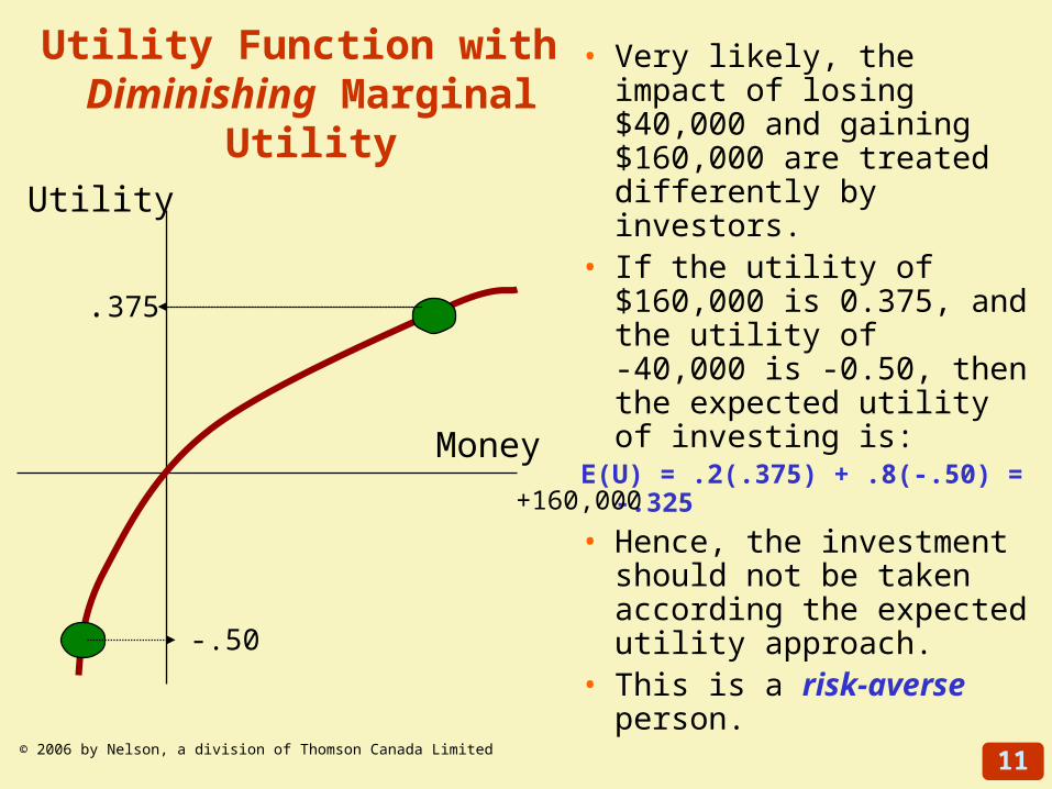
Utility Function with Diminishing Marginal Utility

• Very likely, the impact of losing $40,000 and gaining $160,000 are treated differently by investors.

• If the utility of $160,000 is 0.375, and the utility of -40,000 is -0.50, then the expected utility of investing is:

E(U) = .2(.375) + .8(-.50) = -.325

• Hence, the investment should not be taken according the expected utility approach.

• This is a risk-averse person.

-40,000 +160,000

.375

-.50

Utility

Money


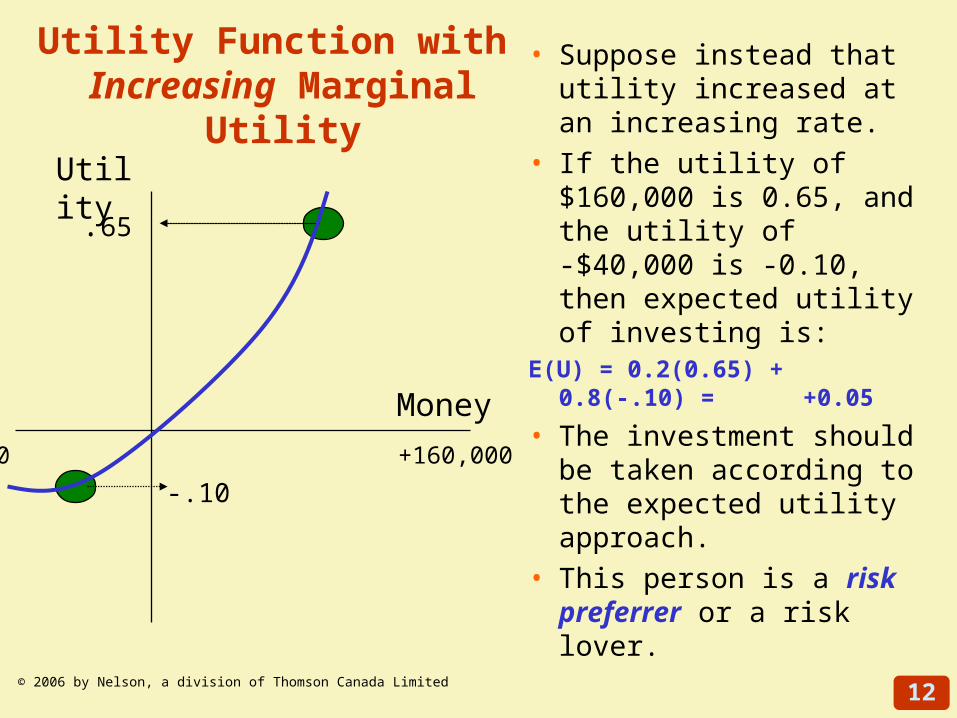
Utility Function with Increasing Marginal Utility

• Suppose instead that utility increased at an increasing rate.

• If the utility of $160,000 is 0.65, and the utility of -$40,000 is -0.10, then expected utility of investing is:

E(U) = 0.2(0.65) + 0.8(-.10) =

+0.05

• The investment should be taken according to the expected utility approach.

• This person is a risk preferrer or a risk lover.

-40,000 +160,000

.65

-.10

Utility

Money


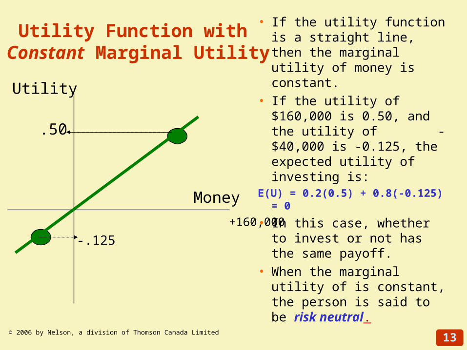
Utility Function with Constant Marginal Utility

• If the utility function is a straight line, then the marginal utility of money is constant.

• If the utility of $160,000 is 0.50, and the utility of -$40,000 is -0.125, the expected utility of investing is:

E(U) = 0.2(0.5) + 0.8(-0.125) = 0

• In this case, whether to invest or not has the same payoff.

• When the marginal utility of is constant, the person is said to be risk neutral.

-40,000 +160,000

.50

-.125

Utility

Money


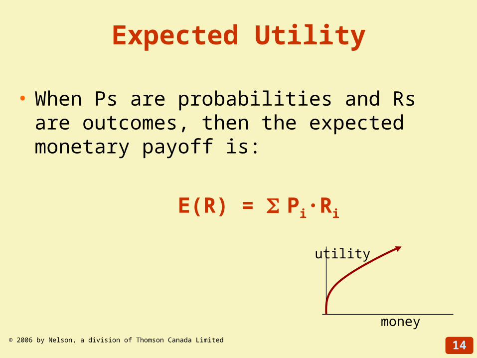
• When Ps are probabilities and Rs are outcomes, then the expected monetary payoff is:

E(R) = Pi·Ri

money

utility

Expected Utility


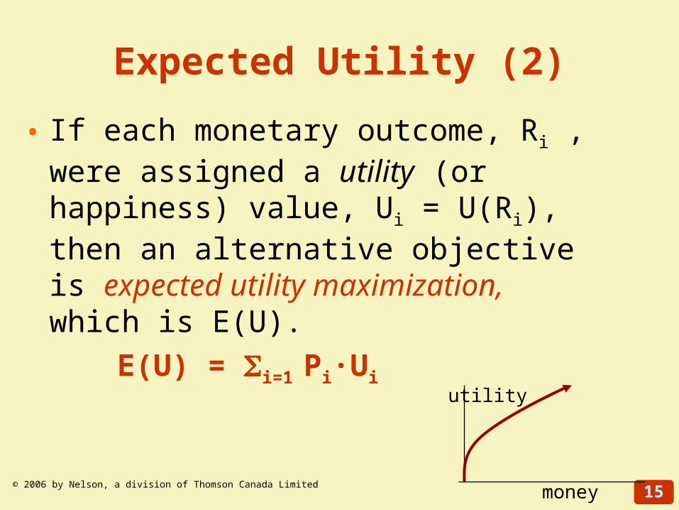
• If each monetary outcome, Ri , were assigned a utility (or happiness) value, Ui = U(Ri), then an alternative objective is expected utility maximization, which is E(U).

E(U) = i=1 Pi·Ui

money

utility

Expected Utility (2)


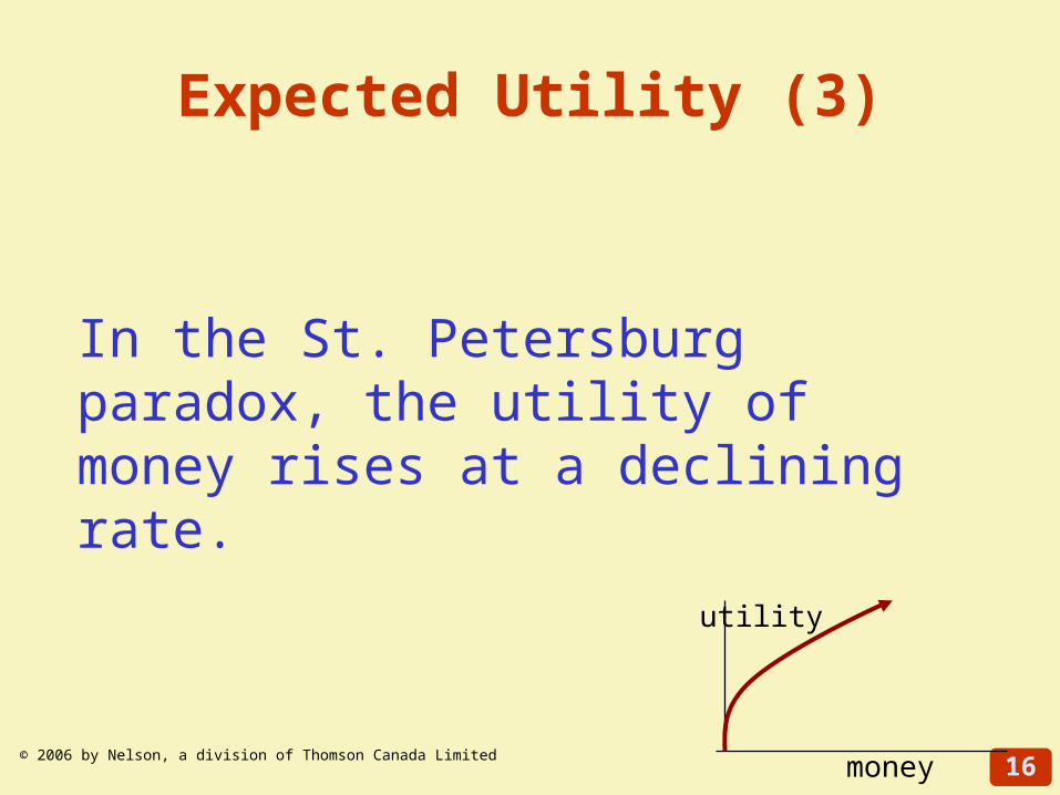
In the St. Petersburg paradox, the utility of money rises at a declining rate.

money

utility

Expected Utility (3)


Should You Move Your Firm to Mexico?

• If successful, the payoff is $10 million with a 68% chance of success.

• If unsuccessful, the payoff is a LOSS of $8.8 million.

• See next slide:


Should You Move Your Firm to Mexico?

• The expected value of the Mexican move is 0.68 (10 million) + 0.32 (-8.8 million) = +$3.984 million.

• The utility of success and failure, respectively, is: +2000 and -4800.

• But the expected utility of the move is 0.68 (2,000) + 0.32 (-4,800) = - 176.

• According to the expected marginal utility approach, the firm should not and will not make the move because it leads to a negative expected utility.


2. Prospect Theory

• Sometimes investors are BOTH risk averse (so that they purchase insurance) and risk preferring (since they like to go to casinos).

• Kahneman and Tversky have suggested that people are risk averse in positively viewed gambles and risk preferring when the gamble is viewed as losing.

• Prospect Theory draws an S-shaped utility function.


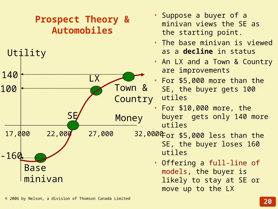
Prospect Theory & Automobiles• Suppose a buyer of a minivan

views the SE as the starting point.

• The base minivan is viewed as a decline in status

• An LX and a Town & Country are improvements

• For $5,000 more than the SE, the buyer gets 100 utiles

• For $10,000 more, the buyer gets only 140 more utiles

• For $5,000 less than the SE, the buyer loses 160 utiles

• Offering a full-line of models, the buyer is likely to stay at SE or move up to the LX

17,000 22,000 27,000 32,0000

100

-160

Utility

Money

LX

SE

Base minivan

Town &Country

140


Prospect Theory & Full Line Forcing

• If a firm offers two qualities of its product (good and better), the buyer picks between them. Let’s suppose 50:50

• If a firm offers third quality (good, better, best), more of the buyers move up, to better and some to best.


Prospect Theory & Full Line Forcing

• As people move through their life cycle, they tend to trade up to the best.» In slide on minivans, suppose that utility of the SE is 320.

» A move down to the base model loses 160 out of 320, or half the utility for a savings of $5,000. This does not seem worth it.

» A move up to the LX gains 100 utiles beyond 320, or a 31% increase in utility for just $5,000.

• Prospect Theory also explains why CEOs like to lump all of the bad news in one quarterly report. Two separate notices of bad news is worse than one announcement of both bad outcomes.


3. Decision Trees

• A decision tree helps to consider the various outcomes over time.

• Each diamond is a decision node, and circles with N are used to designate the impact of the state of nature on that decision.

• Suppose that you must decide whether or not to invest using the same payoffs as on slide 9.

• This can be written in a decision tree.


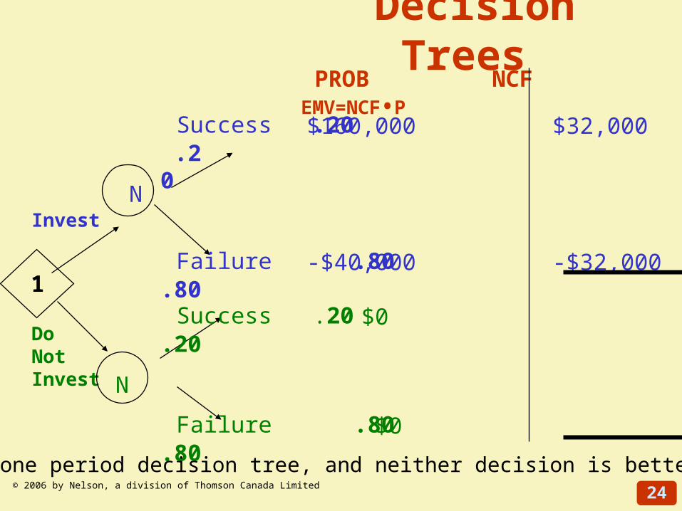
Decision Trees

1

N

N

Success .20

Failure .80

Success .20

Failure .80

.20

.80

.20

.80

PROB NCF EMV=NCF•P

$160,000 $32,000

-$40,000 -$32,000 $0 $0 $0

$0 $0 $0

Invest

Do Not Invest

This is a one period decision tree, and neither decision is better.


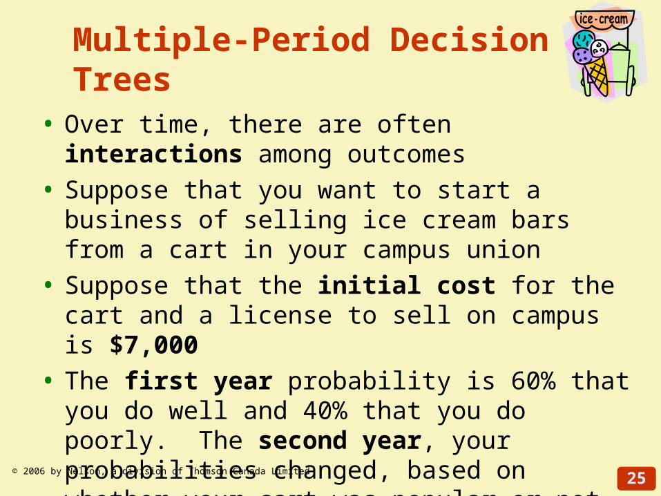
Multiple-Period Decision Trees

• Over time, there are often interactions among outcomes

• Suppose that you want to start a business of selling ice cream bars from a cart in your campus union

• Suppose that the initial cost for the cart and a license to sell on campus is $7,000

• The first year probability is 60% that you do well and 40% that you do poorly. The second year, your probabilities changed, based on whether your cart was popular or not.

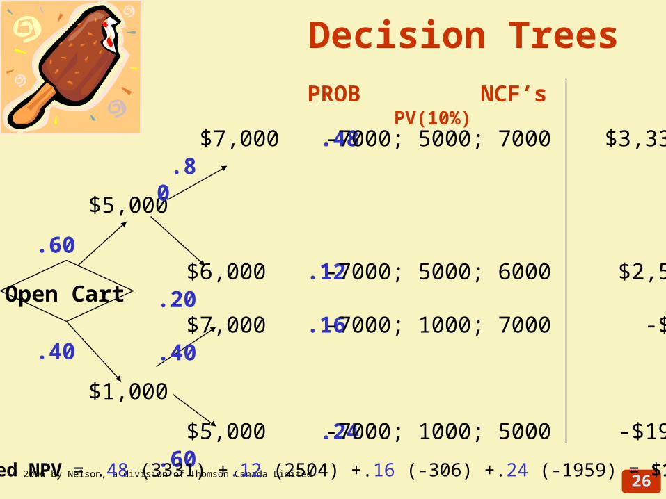
• In this example, you should open a mobile cart, as the expected NPV is +$1,380.


Decision Trees

Open Cart

.60

.40

$5,000

$1,000

$7,000 .48

$6,000 .12

$7,000 .16

$5,000 .24

.80

.20

.40

.60

PROB NCF’s PV(10%)

-7000; 5000; 7000 $3,331

-7000; 5000; 6000 $2,504

-7000; 1000; 7000 -$306

-7000; 1000; 5000 -$1959

Expected NPV = .48 (3331) +.12 (2504) +.16 (-306) +.24 (-1959) = $1,380


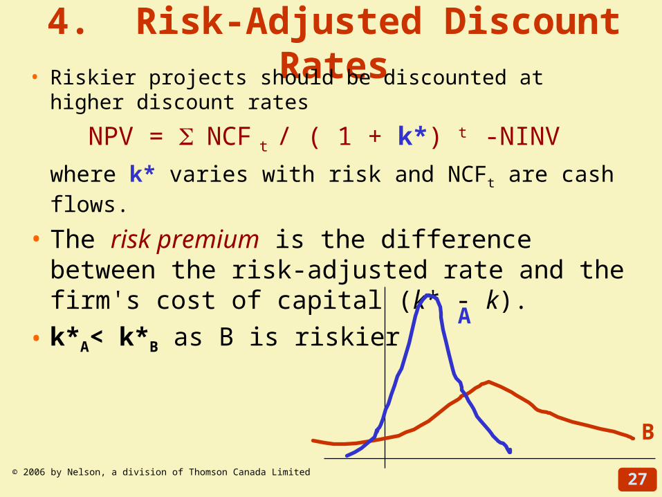
4. Risk-Adjusted Discount Rates• Riskier projects should be discounted at higher discount rates

NPV = NCFt / ( 1 + k*) t -NINV

where k* varies with risk and NCFt are cash flows.

• The risk premium is the difference between the risk-adjusted rate and the firm's cost of capital (k* - k).

• k*A< k*B as B is riskier

B

A


Sources of Risk-Adjusted Discount Rates

• Market-based rates» The magnitude of k*depends on the project.

» Sometimes information on costs of capital in industries similar to this project can be used.

» Look at equivalent risky projects, use that rate

» Is it like a Bond, a Share, or Venture Capital?


Sources of Risk-Adjusted Discount Rates

• Subjective rate» For totally new product lines; however, the selection of

the appropriate risk-adjusted discount rate is subjective. Analysts should be aware that those who advocate the project would want a low discount rate, whereas those who are opposed will feel that a higher rate is warranted.

• Capital Asset Pricing Model (CAPM)» Project’s “beta” and the market return


5. Simulation Approach

• The risks in a decision come from variability of the number of units sold, the price, and costs. With computers, it is possible to estimate cash flows using probability distributions and find the NPV, and to do it over and over again.

NCFt = [q(p) – q(c+s) – D](1-t) + D

» where q(p) is revenue (quantity times price); » q(c+s) is cost (both for production, c, and for selling, s) » and D and t are depreciation and taxes, respectively.


5. Simulation Approach (2)

• If the NPV of each simulation is predominately in the positive range, then the project should be undertaken.

• If the NPV are mostly negative, then the project should be avoided.


Decision Making Under Uncertainty

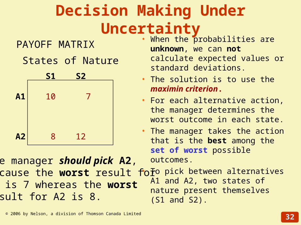
• When the probabilities are unknown, we can not calculate expected values or standard deviations.

• The solution is to use the maximin criterion.

• For each alternative action, the manager determines the worst outcome in each state.

• The manager takes the action that is the best among the set of worst possible outcomes.

• To pick between alternatives A1 and A2, two states of nature present themselves (S1 and S2).

S1 S2

A1 10 7

A2 8 12

The manager should pick A2, because the worst result for A1 is 7 whereas the worst result for A2 is 8.

States of Nature

PAYOFF MATRIX


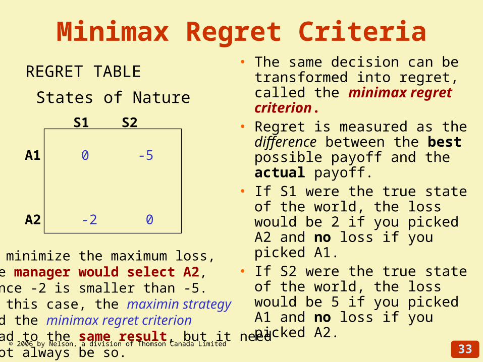
Minimax Regret Criteria• The same decision can be

transformed into regret, called the minimax regret criterion.

• Regret is measured as the difference between the best possible payoff and the actual payoff.

• If S1 were the true state of the world, the loss would be 2 if you picked A2 and no loss if you picked A1.

• If S2 were the true state of the world, the loss would be 5 if you picked A1 and no loss if you picked A2.

S1 S2

A1 0 -5

A2 -2 0

To minimize the maximum loss, the manager would select A2, since -2 is smaller than -5. In this case, the maximin strategy and the minimax regret criterion lead to the same result, but it need not always be so.

States of Nature

REGRET TABLE


Managing Risk and Uncertainty

• In risky situations, managers tend to ask for more information.

• In part, this is a stall for time. But this may mean trying to "test market" the product to learn more.

• It may mean hiring the expert opinion of others.

• Firms hire outside lawyers, accountants, economists, and others to gauge the situation.

• Credit rating services, such as DBRS, sell information to manage risk.


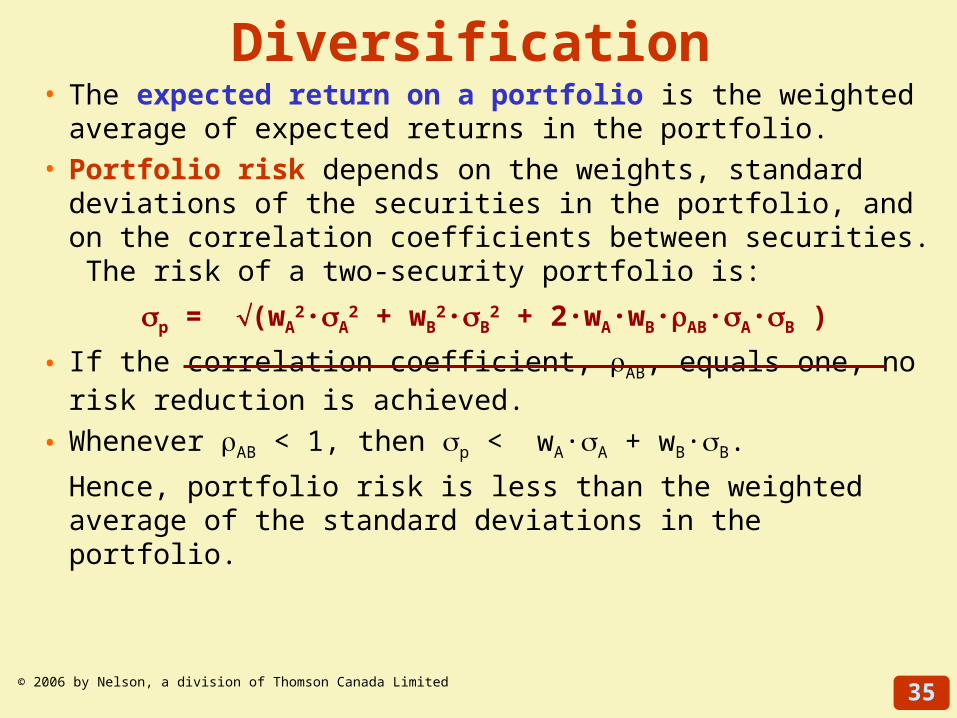
Diversification • The expected return on a portfolio is the weighted average of

expected returns in the portfolio. • Portfolio risk depends on the weights, standard deviations of

the securities in the portfolio, and on the correlation coefficients between securities. The risk of a two-security portfolio is:

p = (wA2·A

2 + wB2·B

2 + 2·wA·wB·AB·A·B )

• If the correlation coefficient, AB, equals one, no risk reduction is achieved.

• Whenever AB < 1, then p < wA·A + wB·B.

Hence, portfolio risk is less than the weighted average of the standard deviations in the portfolio.


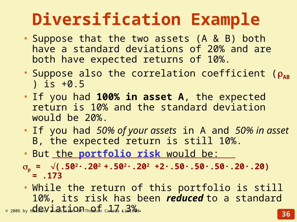
Diversification Example• Suppose that the two assets (A & B) both have a

standard deviations of 20% and are both have expected returns of 10%.

• Suppose also the correlation coefficient (AB ) is +0.5• If you had 100% in asset A, the expected return is 10%

and the standard deviation would be 20%.• If you had 50% of your assets in A and 50% in asset B,

the expected return is still 10%.• But the portfolio risk would be:p = (.502·.202 +.502·.202 +2·.50·.50·.50·.20·.20) = .173

• While the return of this portfolio is still 10%, its risk has been reduced to a standard deviation of 17.3%.


Other Approaches for Managing Risk & Uncertainty

• Hedging – limiting risk by making an offsetting investment. Investing in securities that are negatively correlated provides hedging benefits.

• Insurance – pay a premium to avoid bad outcomes (fire, theft, accidents by chief officers, etc. )

• Gaining control over the operating environment – invest in suppliers to assure continuance of service

• Limited use of firm-specific assets – non-redeployable assets are riskier.

• Scenario Planning – being ready for the unexpected and determining your response to it

Documents

1 © 2006 by Nelson, a division of Thomson Canada Limited Slides developed by: William Rentz & Al Kahl University of Ottawa Web Chapter 19 Decisions Under