SIMG-716Linear Imaging Mathematics I, Handout 06

1 2-D Special Functions• Function of two independent spatial variables specifies amplitude (“brightness”) at each spatialcoordinate in a plane

— fulfill usual definition of “image”.

• Three categories:

1. Cartesian separable functions

— represented as products of 1-D special functions along orthogonal Cartesian axes

2. Circularly symmetric functions

— product of 1-D functions in radial direction and unit constant in orthogonal (“az-imuthal”) direction

3. General functions

— includes pictorial scenes and 2-D stochastic functions.

2 2-D Separable Functions• “orthogonal multiplication” of two 1-D functions fx [x] and fy [y]:

f [x, y] = fx [x]× fy [y]

• General expression for separable function in terms of scaled and translated 1-D functions is:

f [x, y] = fx

∙x− x0

a

¸× fy

∙y − y0

b

¸— a and b are real-valued scale factors

— x0 and y0 are real-valued translation parameters

• Consider those which have general application to imaging problems.

• Volume of 2-D separable function is product of areas of component 1-D functions:ZZ +∞

−∞f [x, y] dx dy =

ZZ +∞

−∞fx

∙x− x0

a

¸fy

∙y − y0

b

¸dx dy

=

µZ +∞

−∞fx

∙x− x0

a

¸dx

¶µZ +∞

−∞fy

∙y − y0

b

¸dy

¶

1

2.1 Rotations of 2-D Separable Functions

• Example: square centered at origin with sides parallel to the x- and y-axes rotated by ±π4 to

generate “baseball diamond” with vertices on x - and y-axes

• Rotation of function about origin is an “imaging system” with 2-D input function f [x, y] and2-D output g [x, y]

— Amplitude g of rotated function at [x, y] is original amplitude f at location [x0, y0]:

O{f [x, y]} = g [x, y] = f [x0, y0]

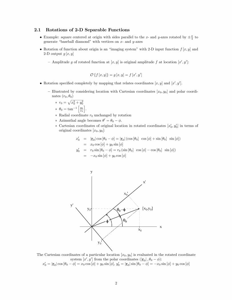
• Rotation specified completely by mapping that relates coordinates [x, y] and [x0, y0].

— Illustrated by considering location with Cartesian coordinates [x0, y0] and polar coordi-nates (r0, θ0)

∗ r0 =px20 + y20

∗ θ0 = tan−1hy0x0

i.

∗ Radial coordinate r0 unchanged by rotation∗ Azimuthal angle becomes θ0 = θ0 − φ.∗ Cartesian coordinates of original location in rotated coordinates [x00, y00] in terms oforiginal coordinates [x0, y0]:

x00 = |r0| cos [θ0 − φ] = |r0| (cos [θ0] cos [φ] + sin [θ0] sin [φ])= x0 cos [φ] + y0 sin [φ]

y00 = r0 sin [θ0 − φ] = r0 (sin [θ0] cos [φ]− cos [θ0] sin [φ])= −x0 sin [φ] + y0 cos [φ]

The Cartesian coordinates of a particular location [x0, y0] is evaluated in the rotated coordinatesystem [x0, y0] from the polar coordinates (|r0| , θ0 − φ):

x00 = |r0| cos [θ0 − φ] = x0 cos [φ] + y0 sin [φ], y00 = |r0| sin [θ0 − φ] = −x0 sin [φ] + y0 cos [φ]

2

2.2 Rotated Coordinates as Scalar Products

• Rotated x -coordinate written as scalar product of position vector r ≡ [x, y] and unit vectordirected along azimuth angle φ, which has Cartesian coordinates [cos [φ] , sin [φ]], denoted bybp:

x0 = x cos [φ] + y sin [φ] =

∙xy

¸•∙cos [φ]sin [φ]

¸≡ r • bp

• Notation for x0 may seem “weird” because rotated 1-D argument x0 is function of both x andy through scalar product of two vectors.

— rotated argument x0 defines a set of points r = [x, y] that fulfill same conditions ascoordinate x in original function.

— Rotated coordinate x0 evaluates to 0 for all vectors r ⊥ bp, (equivalent to r • bp = 0).— Vectors r specified by condition r • bp = 0 include coordinates on “both” sides of origin— Complete set of possible azimuth angles specified by angles φ in interval spanning πradians, e.g., −π

2 ≤ φ < +π2 . This means that the set of possible rotations is specified by

unit vectors bp in the first and fourth quadrants.• Polar form of position vector r = (|r| , θ) = (r, θ) substituted into scalar product in terms ofmagnitudes of vectors and included angle:

r • bp = |r| ¯̄bp¯̄ cos [θ − φ] = r cos [θ − φ] because¯̄bp¯̄ = 1.

• y-coordinate of rotated function written in same way as scalar product of position vector rand unit vector directed along azimuth angle φ+ π

2 ;call it bp⊥:y0 = x cos

hφ+

π

2

i+ y sin

hφ+

π

2

i= −x sin [φ] + y cos [φ] =

∙xy

¸•∙− sin [φ]cos [φ]

¸≡ r • bp⊥

• Polar form for rotated y-axis is:

r • bp⊥ = |r|¯̄bp¯̄ cos hθ − ³φ+ π

2

´i= r cos

hθ − φ− π

2

i= r sin [θ − φ]

g [x, y] = fx [x0] fy [y

0] = fx£r • bp¤ fy

hr • bp⊥i

• Formula is applicable to any 2-D separable special function

3

3 Definitions of 2-D Separable Functions

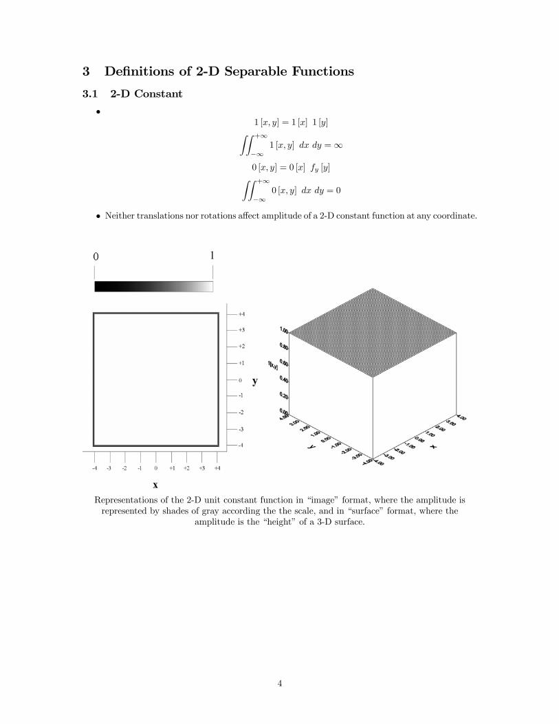
3.1 2-D Constant

•1 [x, y] = 1 [x] 1 [y]ZZ +∞

−∞1 [x, y] dx dy =∞

0 [x, y] = 0 [x] fy [y]ZZ +∞

−∞0 [x, y] dx dy = 0

• Neither translations nor rotations affect amplitude of a 2-D constant function at any coordinate.

Representations of the 2-D unit constant function in “image” format, where the amplitude isrepresented by shades of gray according the the scale, and in “surface” format, where the

amplitude is the “height” of a 3-D surface.

4

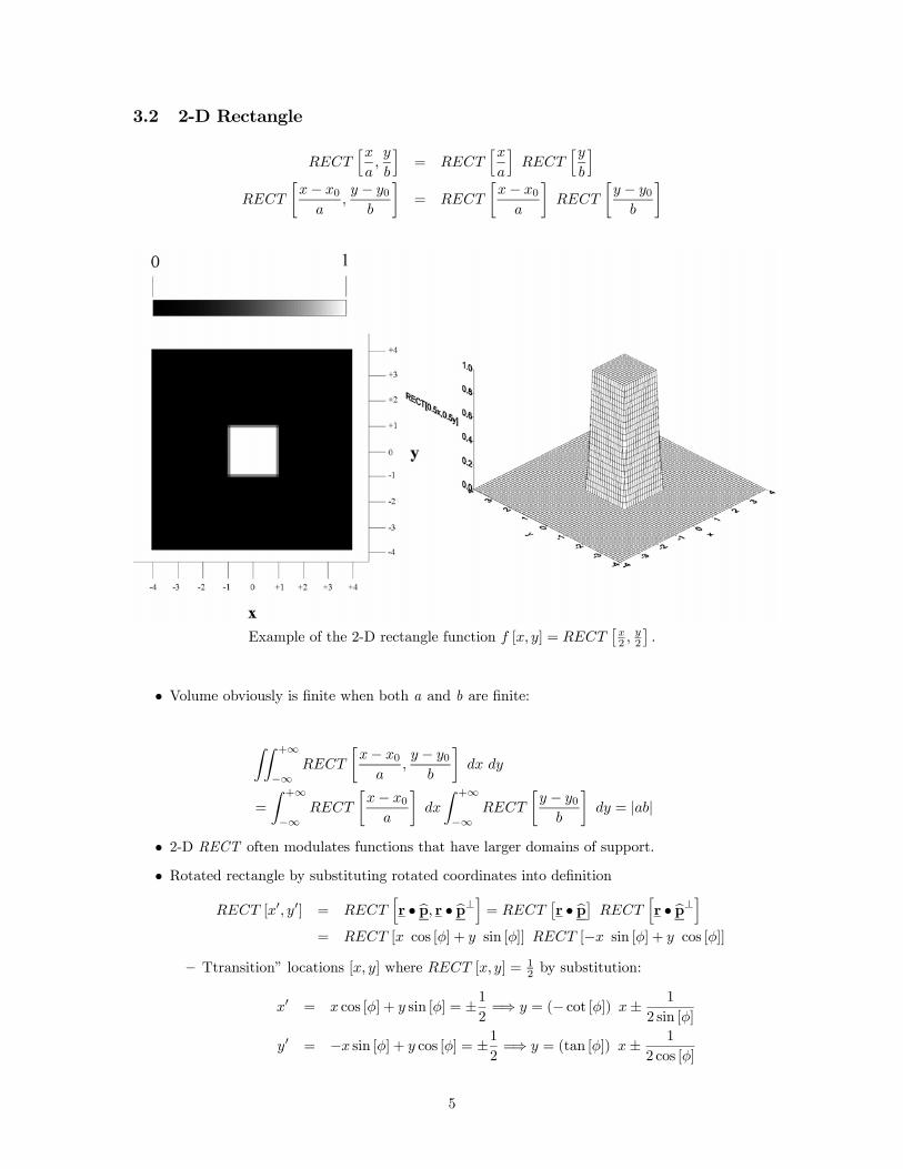
3.2 2-D Rectangle

RECThxa,y

b

i= RECT

hxa

iRECT

hyb

iRECT

∙x− x0

a,y − y0

b

¸= RECT

∙x− x0

a

¸RECT

∙y − y0

b

¸

Example of the 2-D rectangle function f [x, y] = RECT£x2 ,

y2

¤.

• Volume obviously is finite when both a and b are finite:

ZZ +∞

−∞RECT

∙x− x0

a,y − y0

b

¸dx dy

=

Z +∞

−∞RECT

∙x− x0

a

¸dx

Z +∞

−∞RECT

∙y − y0

b

¸dy = |ab|

• 2-D RECT often modulates functions that have larger domains of support.

• Rotated rectangle by substituting rotated coordinates into definition

RECT [x0, y0] = RECThr • bp, r • bp⊥i = RECT

£r • bp¤ RECT

hr • bp⊥i

= RECT [x cos [φ] + y sin [φ]] RECT [−x sin [φ] + y cos [φ]]

— Ttransition” locations [x, y] where RECT [x, y] = 12 by substitution:

x0 = x cos [φ] + y sin [φ] = ±12=⇒ y = (− cot [φ]) x± 1

2 sin [φ]

y0 = −x sin [φ] + y cos [φ] = ±12=⇒ y = (tan [φ]) x± 1

2 cos [φ]

5

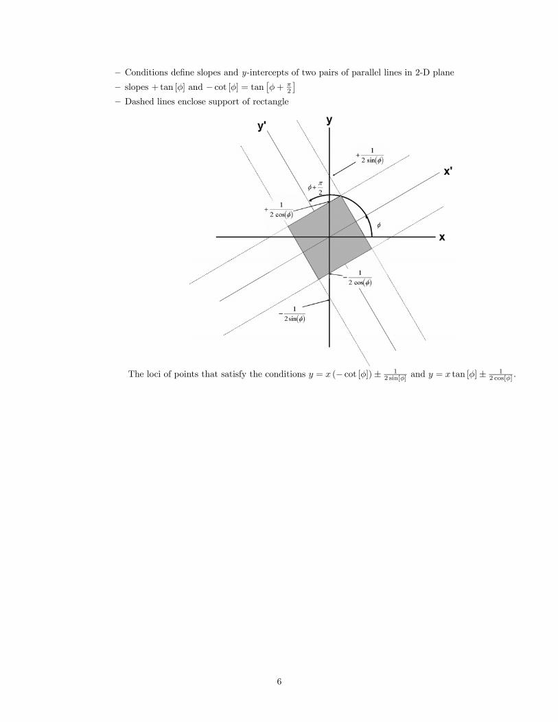
— Conditions define slopes and y-intercepts of two pairs of parallel lines in 2-D plane

— slopes +tan [φ] and − cot [φ] = tan£φ+ π

2

¤— Dashed lines enclose support of rectangle

The loci of points that satisfy the conditions y = x (− cot [φ])± 12 sin[φ] and y = x tan [φ]± 1

2 cos[φ] .

6

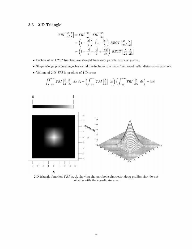
3.3 2-D Triangle

TRIhxa,y

b

i= TRI

hxa

iTRI

hyb

i=

µ1− |x|

a

¶ µ1− |y|

b

¶RECT

h x2a

,y

2b

i=

µ1− |x|

a− |y|

b+|xy|ab

¶RECT

h x2a

,y

2b

i• Profiles of 2-D TRI function are straight lines only parallel to x- or y-axes.

• Shape of edge profile along other radial line includes quadratic function of radial distance=⇒parabola.

• Volume of 2-D TRI is product of 1-D areas:ZZ +∞

−∞TRI

hxa,y

b

idx dy =

µZ +∞

−∞TRI

hxb

idx

¶µZ +∞

−∞TRI

hyb

idy

¶= |ab|

2-D triangle function TRI [x, y], showing the parabolic character along profiles that do notcoincide with the coordinate axes.

7

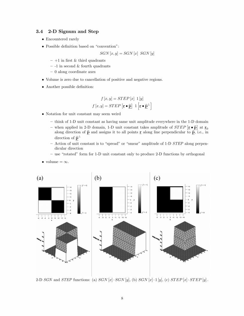
3.4 2-D Signum and Step

• Encountered rarely

• Possible definition based on “convention”:SGN [x, y] = SGN [x] SGN [y]

— +1 in first & third quadrants— -1 in second & fourth quadrants— 0 along coordinate axes

• Volume is zero due to cancellation of positive and negative regions.

• Another possible definition:

f [x, y] = STEP [x] 1 [y]

f [x, y] = STEP£r • bp¤ 1 hr • bp⊥i

• Notation for unit constant may seem weird

— think of 1-D unit constant as having same unit amplitude everywhere in the 1-D domain— when applied in 2-D domain, 1-D unit constant takes amplitude of STEP

£r • bp¤ at r0

along direction of bp and assigns it to all points r along line perpendicular to bp, i.e., indirection of bp⊥

— Action of unit constant is to “spread” or “smear” amplitude of 1-D STEP along perpen-dicular direction

— use “rotated” form for 1-D unit constant only to produce 2-D functions by orthogonal

• volume =∞.

2-D SGN and STEP functions: (a) SGN [x] ·SGN [y], (b) SGN [x] · 1 [y], (c) STEP [x] ·STEP [y] .

8

3.5 2-D SINC

SINChxa,y

b

i= SINC

hxa

iSINC

hyb

i=sin£πxa

¤sin£πyb

¤¡πxa

¢ ¡πyb

¢• Amplitude> 0 in regions where both of 1-D functions are positive or both are negative

• Amplitude < 0 where either (but not both) is negative.

• “checkerboard-like” pattern of positive and negative regions

• volume is product of the areas of the individual functions:ZZ +∞

−∞SINC

hxa,y

b

idx dy =

µZ +∞

−∞SINC

hxa

idx

¶µZ +∞

−∞SINC

hyb

idy

¶= |a| |b| = |ab|

SINC [x, y] = SINC [x] · SINC [y]

9

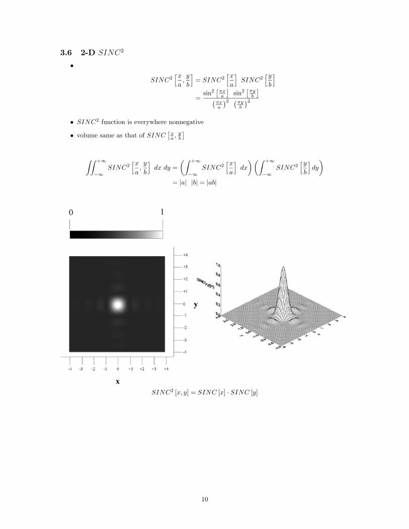
3.6 2-D SINC2

•

SINC2hxa,y

b

i= SINC2

hxa

iSINC2

hyb

i=sin2

£πxa

¤sin2

£πyb

¤¡πxa

¢2 ¡πyb

¢2• SINC2 function is everywhere nonnegative

• volume same as that of SINC£xa ,

yb

¤ZZ +∞

−∞SINC2

hxa,y

b

idx dy =

µZ +∞

−∞SINC2

hxa

idx

¶µZ +∞

−∞SINC2

hyb

idy

¶= |a| |b| = |ab|

SINC2 [x, y] = SINC [x] · SINC [y]

10

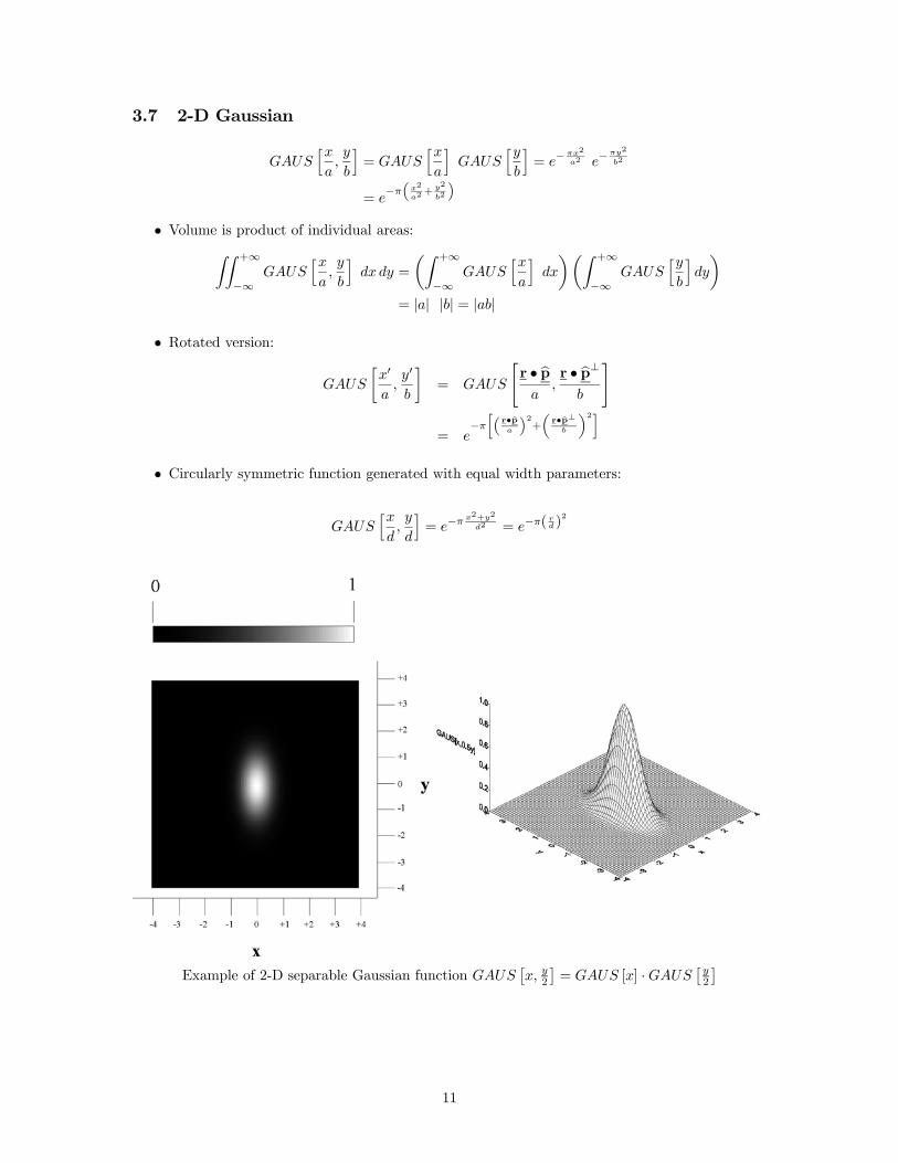
3.7 2-D Gaussian

GAUShxa,y

b

i= GAUS

hxa

iGAUS

hyb

i= e−

πx2

a2 e−πy2

b2

= e−π x2

a2+y2

b2

• Volume is product of individual areas:ZZ +∞

−∞GAUS

hxa,y

b

idx dy =

µZ +∞

−∞GAUS

hxa

idx

¶µZ +∞

−∞GAUS

hyb

idy

¶= |a| |b| = |ab|

• Rotated version:

GAUS

∙x0

a,y0

b

¸= GAUS

"r • bpa

,r • bp⊥

b

#

= e−π r•p

a

2+

r•p⊥b

2

• Circularly symmetric function generated with equal width parameters:

GAUShxd,y

d

i= e−π

x2+y2

d2 = e−π(rd )

2

Example of 2-D separable Gaussian function GAUS£x, y2

¤= GAUS [x] ·GAUS

£y2

¤

11

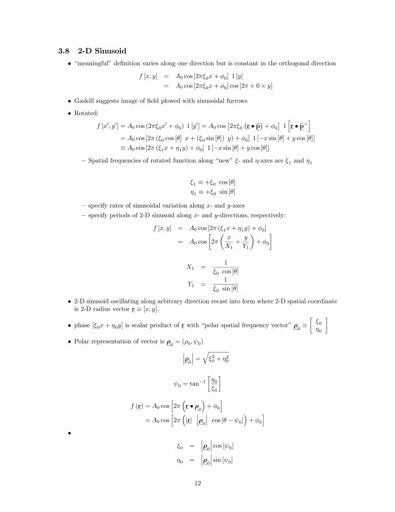
3.8 2-D Sinusoid

• “meaningful” definition varies along one direction but is constant in the orthogonal direction

f [x, y] = A0 cos [2πξ0x+ φ0] 1 [y]

= A0 cos [2πξ0x+ φ0] cos [2π × 0× y]

• Gaskill suggests image of field plowed with sinusoidal furrows

• Rotated:

f [x0, y0] = A0 cos (2πξ0x0 + φ0) 1 [y

0] = A0 cos£2πξ0

¡r • bp¢+ φ0

¤1hr • bp⊥i

= A0 cos [2π (ξ0 cos [θ] x+ (ξ0 sin [θ]) y) + φ0] 1 [−x sin [θ] + y cos [θ]]

≡ A0 cos [2π (ξ1x+ η1y) + φ0] 1 [−x sin [θ] + y cos [θ]]

— Spatial frequencies of rotated function along “new” ξ- and η-axes are ξ1 and η1

ξ1 ≡ +ξ0 cos [θ]η1 ≡ +ξ0 sin [θ]

— specify rates of sinusoidal variation along x- and y-axes

— specify periods of 2-D sinusoid along x- and y-directions, respectively:

f [x, y] = A0 cos [2π (ξ1x+ η1y) + φ0]

= A0 cos

∙2π

µx

X1+

y

Y1

¶+ φ0

¸

X1 =1

ξ0 cos [θ]

Y1 =1

ξ0 sin [θ]

• 2-D sinusoid oscillating along arbitrary direction recast into form where 2-D spatial coordinateis 2-D radius vector r ≡ [x, y].

• phase [ξ0x+ η0y] is scalar product of r with “polar spatial frequency vector” ρ0 ≡∙ξ0η0

¸• Polar representation of vector is ρ

0= (ρ0, ψ0)¯̄̄

ρ0

¯̄̄=

qξ20 + η20

ψ0 = tan−1∙η0ξ0

¸

f (r) = A0 cosh2π³r • ρ

0

´+ φ0

i= A0 cos

h2π³|r|

¯̄̄ρ0

¯̄̄cos [θ − ψ0]

´+ φ0

i•

ξ0 =¯̄̄ρ0

¯̄̄cos [ψ0]

η0 =¯̄̄ρ0

¯̄̄sin [ψ0]

12

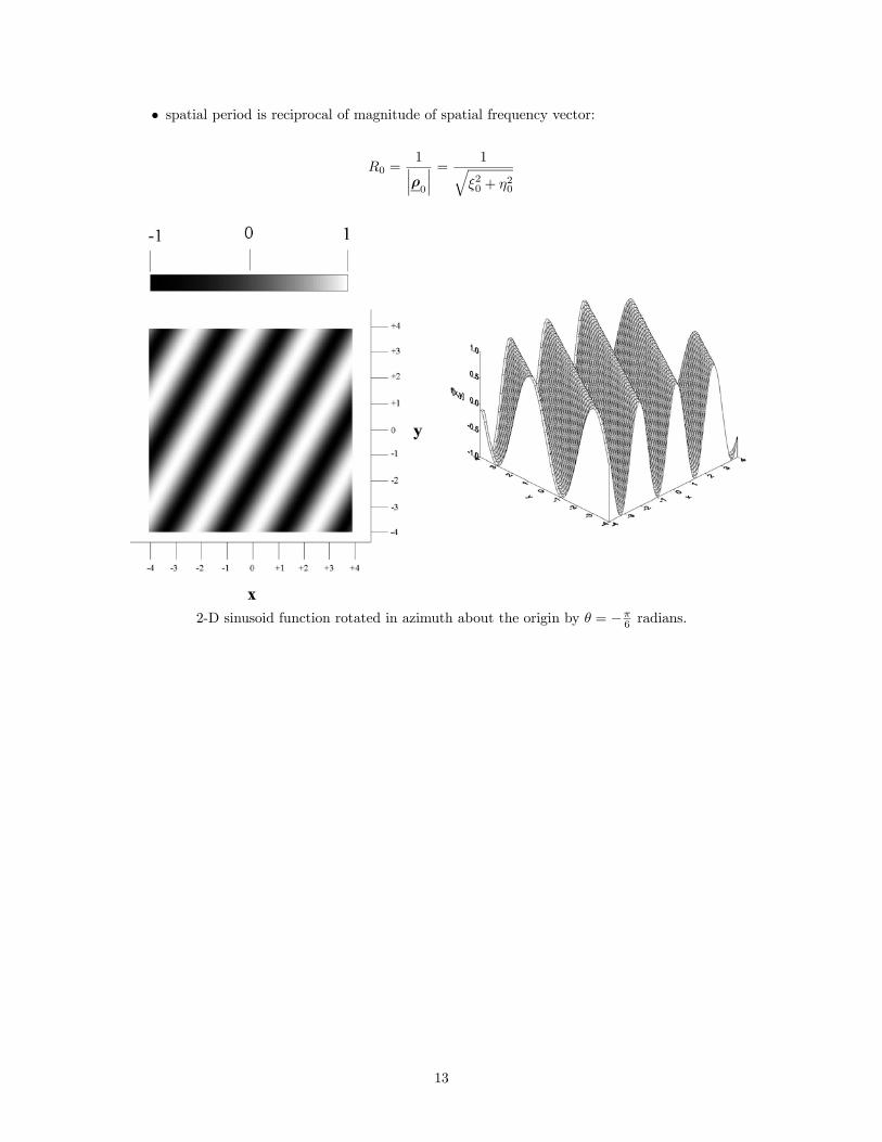
• spatial period is reciprocal of magnitude of spatial frequency vector:

R0 =1¯̄̄ρ0

¯̄̄ = 1qξ20 + η20

2-D sinusoid function rotated in azimuth about the origin by θ = −π6 radians.

13

4 2-D Dirac Delta Function and its Relatives• Several flavors of 2-D Dirac delta function possible

— different separable versions of 2-D Dirac delta function defined in Cartesian and polarcoordinates

• Properties:δ [x− x0, y − y0] = 0 for x− x0 6= 0 or y − y0 6= 0ZZ +∞

−∞δ [x− x0, y − y0] dx dy = 1

• Expressed as limit of sequence of 2-D functions, each with unit volume

• May be generated from 2-D RECT, TRI, GAUS, SINC, and SINC 2 in Cartesian coordinates

• Separability of functions ensures that corresponding representation of δ [x, y] is separable

• Most common representation of δ [x, y] based on 2-D RECT function of unit volume in thelimit of infinitesimal area:

δ [x, y] = limb→0

limd→0

½1

bdRECT

hxb,y

d

i¾= lim

b→0

½1

bRECT

hxb

i¾× lim

d→0

½1

dRECT

hyd

i¾4.1 Properties of Separable 2-D Dirac Delta Function, Cartesian Coor-

dinates

δ [x, y] = δ [x] δ [y]

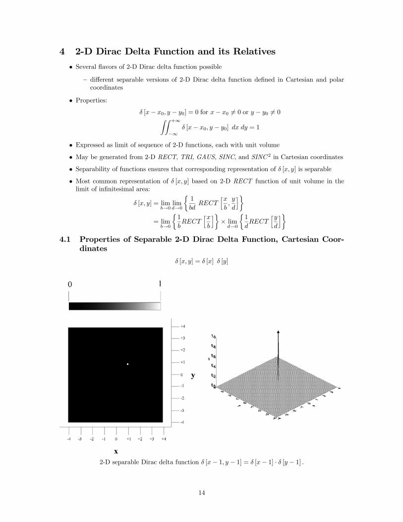
2-D separable Dirac delta function δ [x− 1, y − 1] = δ [x− 1] · δ [y − 1] .

14

• 2-D Dirac delta function may be synthesized by summing unit-amplitude 2-D complex linear-phase exponentials with all spatial frequencies.

δ [x]× δ [y] =

µZ +∞

−∞e+2πiξxdξ

¶µZ +∞

−∞e+2πiηydη

¶=

ZZ +∞

−∞e+2πiξxe+2πiηy dξ dη

=

ZZ +∞

−∞e+2πi(ξx+ηy) dξ dη = δ [x, y]

• Because odd imaginary parts cancel:

δ [x, y] =

ZZ +∞

−∞cos [2π (ξx+ ηy)] dξ dη

• Scaling property of δ [x] =⇒

δhxb,y

d

i= δ

hxb

iδhyd

i= |b| δ [x] |d| δ [y]= |bd| δ [x] δ [y] = |bd| δ [x, y]

• Translat by shifting separable components:

δ

∙x− x0

b,y − y0d

¸= |bd| δ [x− x0] δ [y − y0]

• Sifting property evaluates amplitude at a specific locationZZ +∞

−∞f [x, y] δ [x− x0, y − y0] dxdy = f [x0, y0]

15

4.2 Properties of 2-D Dirac Delta Function, Polar Coordinates

• 2-D Dirac delta function located on x-axis at distance α > 0 from origin

— polar coordinates are r0 = α and θ0 = 0.

δ [x− α, y] = δ [x− α] δ [y]

— Polar representation easy to derive because radial coordinate directed along x-axis

— Azimuthal displacement due to angle parallel to y-axis.

— Identify x→ r, α→ r0, and y → r0θ and substitute directly, use 1-D scaling property

δ [x− α] δ [y] = δ [r − r0] δ [r0θ]

= δ [r − r0]

µ1

|r0|δ [θ]

¶=

δ [r − r0]

r0δ [θ]

• last step follows from observation that polar radial coordinate r0 ≥ 0

• Domain of azimuthal coordinate θ is a continuous interval of 2π radians, e.g., −π ≤ θ < +π

• Generalize for a 2-D Dirac delta function located at same radial distance r0 from the originbut at different azimuth θ0

— Cartesian coordinates x0 = r0 cos [θ0], y0 = r0 sin [θ0]

δ [x− x0, y − y0] = δ [x− r0 cos [θ0]] δ [y − r0 sin [θ0]]

=δ [r − r0]

r0δ [θ − θ0] ≡ δ (r− r0)

— Polar form is product of 1-D Dirac delta functions in the radial and azimuthal directions

— Amplitude scaled by reciprocal of the radial distance.

• Confirm that expression satisfies criteria for 2-D Dirac delta function.

• Easy to show that support is infinitesimal

• Volume is evaluated easily:

ZZ +∞

−∞δ [r− r0] dr =

Z +π

−πdθ

Z +∞

0

µδ [r − r0]

r0δ [θ − θ0]

¶r dr

=

µZ +π

−πδ [θ − θ0] dθ

¶·µZ +∞

0

δ [r − r0]

r0r dr

¶where r0 > 0

= 1 ·Z +∞

0

δ [r − r0]

r0r0 dr = 1 ·

Z +∞

0

δ [r − r0] dr = 1

• Extend derivation of polar form of 2-D Dirac delta function to r0 = 0

δ [r− 0]

• Domain of r is semiclosed single-sided interval [0,+∞)

— 1-D radial part δ (r − r0) at origin cannot be symmetric

— θ0 is indeterminate at origin

16

— not valid for r0 = 0

— 2-D Dirac delta function at the origin must be circularly symmetric and therefore afunction of r only

— No dependence on azimuth angle θ:

δ (r− 0) = α δ [|r|]× 1 [θ]= α δ [r]× 1 [θ]

∗ α is scaling parameter ensures that δ (r) has unit volume

— Domains of polar arguments are 0 ≤ r < +∞ and −π ≤ θ < +π.

— Modify domains

∗ Radial variable over domain (−∞,+∞)∗ Azimuthal domain constrained to interval of π radians, e.g., [0,+π) or

£−π2 ,+

π2

¢.

1 =

Z +π

−π

Z +∞

0

α δ [r] 1 [θ] r dr dθ =

Z +π2

−π2

Z +∞

−∞α δ [r] 1 [θ] r dr dθ

=

Z +π2

−π2

1 [θ] dθ

Z +∞

−∞α δ [r] r dr =

Z +∞

−∞α δ [r] πr dr

— Area of δ (r) over (−∞,+∞) is unity∗ α = (πr)−1.

δ (r− 0) = δ (r)

=

µ1

πr

¶δ (r) 1 [θ]

=δ (r)

πr

17

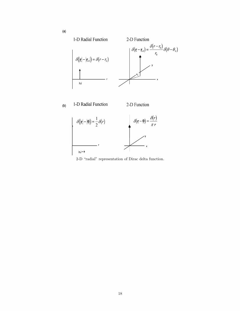
2-D “radial” representation of Dirac delta function.

18

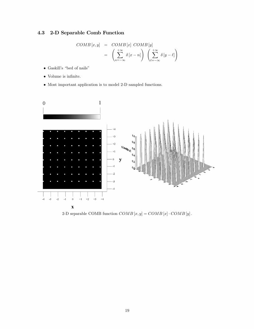
4.3 2-D Separable Comb Function

COMB [x, y] = COMB [x] COMB [y]

=

Ã+∞X

n=−∞δ [x− n]

! Ã+∞X=−∞

δ [y − ]

!

• Gaskill’s “bed of nails”

• Volume is infinite.

• Most important application is to model 2-D sampled functions.

2-D separable COMB function COMB [x, y] = COMB [x] · COMB [y] .

19

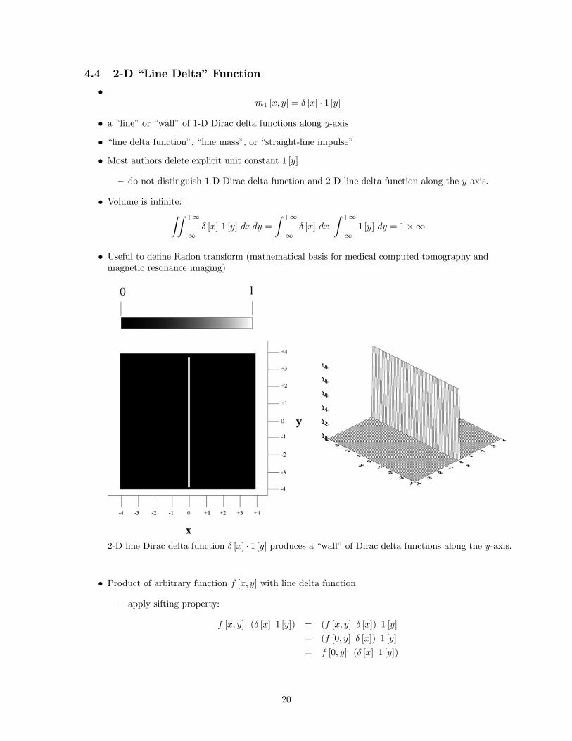
4.4 2-D “Line Delta” Function

•m1 [x, y] = δ [x] · 1 [y]

• a “line” or “wall” of 1-D Dirac delta functions along y-axis

• “line delta function”, “line mass”, or “straight-line impulse”

• Most authors delete explicit unit constant 1 [y]

— do not distinguish 1-D Dirac delta function and 2-D line delta function along the y-axis.

• Volume is infinite:ZZ +∞

−∞δ [x] 1 [y] dx dy =

Z +∞

−∞δ [x] dx

Z +∞

−∞1 [y] dy = 1×∞

• Useful to define Radon transform (mathematical basis for medical computed tomography andmagnetic resonance imaging)

2-D line Dirac delta function δ [x] · 1 [y] produces a “wall” of Dirac delta functions along the y-axis.

• Product of arbitrary function f [x, y] with line delta function

— apply sifting property:

f [x, y] (δ [x] 1 [y]) = (f [x, y] δ [x]) 1 [y]

= (f [0, y] δ [x]) 1 [y]

= f [0, y] (δ [x] 1 [y])

20

• Volume of product of functions is:ZZ +∞

−∞f [x, y] δ [x] 1 [y] dx dy =

ZZ +∞

−∞f [0, y] δ [x] 1 [y] dx dy

=

Z +∞

−∞f [0, y] 1 [y] dy

Z +∞

−∞δ [x] dx

=

Z +∞

−∞f [0, y] dy

• Line delta function δ [x] 1 [y] “sifts out” area of f [x, y] evaluated along the y-axis

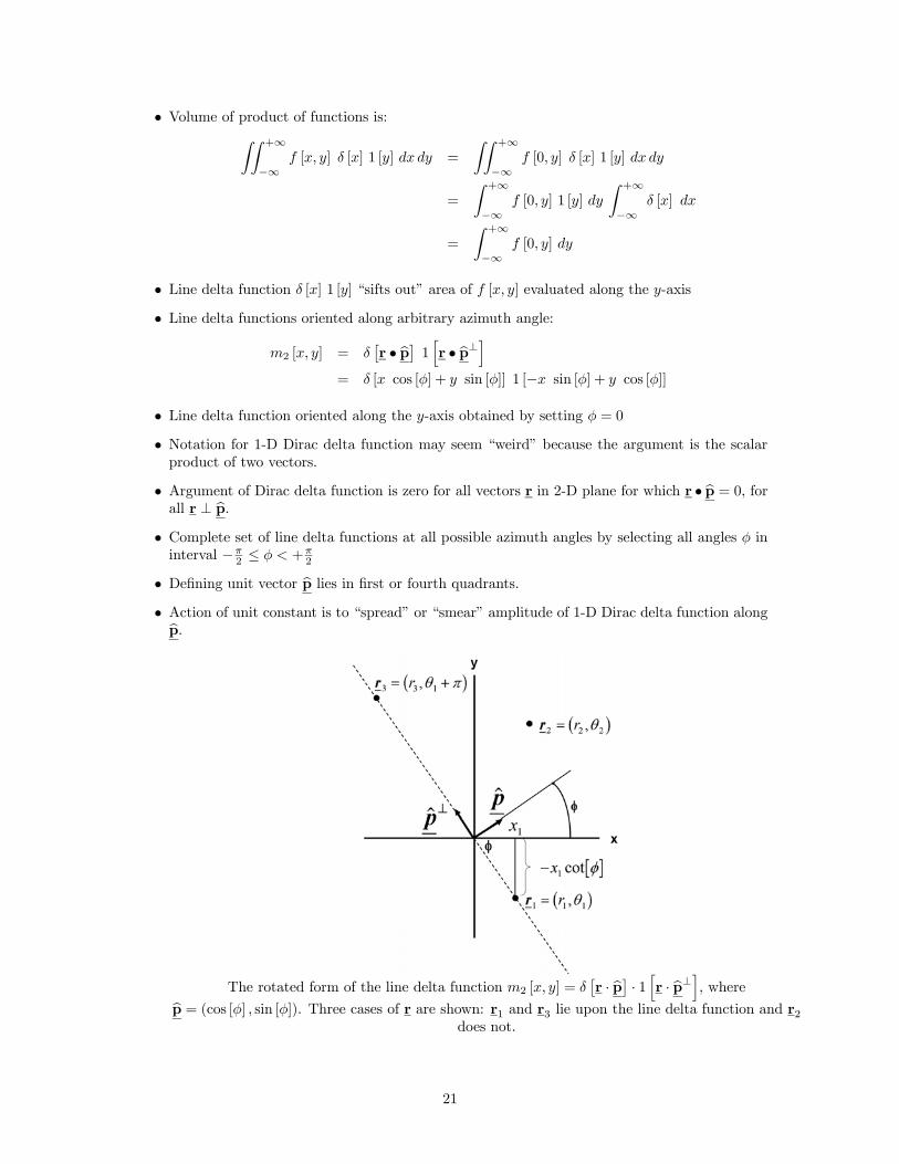
• Line delta functions oriented along arbitrary azimuth angle:

m2 [x, y] = δ£r • bp¤ 1 hr • bp⊥i

= δ [x cos [φ] + y sin [φ]] 1 [−x sin [φ] + y cos [φ]]

• Line delta function oriented along the y-axis obtained by setting φ = 0

• Notation for 1-D Dirac delta function may seem “weird” because the argument is the scalarproduct of two vectors.

• Argument of Dirac delta function is zero for all vectors r in 2-D plane for which r • bp = 0, forall r ⊥ bp.

• Complete set of line delta functions at all possible azimuth angles by selecting all angles φ ininterval −π

2 ≤ φ < +π2

• Defining unit vector bp lies in first or fourth quadrants.• Action of unit constant is to “spread” or “smear” amplitude of 1-D Dirac delta function alongbp.

The rotated form of the line delta function m2 [x, y] = δ£r · bp¤ · 1 hr · bp⊥i, wherebp = (cos [φ] , sin [φ]). Three cases of r are shown: r1 and r3 lie upon the line delta function and r2

does not.

21

• Use polar form of radius vector r = (r, φ), where 0 ≤ r < +∞ and −π ≤ φ < +π

m2 [x, y] = δ£r • bp¤ 1 hr • bp⊥i

= δ£|r|¯̄bp¯̄ cos [θ − φ]

¤1hr • bp⊥i

= δ [|r| cos [θ − φ]] 1hr • bp⊥i

= δ [r cos [φ− θ]]

• Expression determines the set of values of (r, θ) on radial line through origin perpendicular toazimuthal angle φ.

• Write as function of azimuthal angle φ by recasting into more convenient form

— Apply expression for Dirac delta function with a functional argument

δ£r • bp¤ 1 hr • bp⊥i = δ [r cos [θ − φ]] 1

hr • bp⊥i

= δ [g [φ]] 1hr • bp⊥i

=1

|g0 (φ0)|δ [φ− φ0] 1

hr • bp⊥i

=1

r |sin [θ − φ0]|δ [φ− φ0] 1

hr • bp⊥i

— φ0 is angle that satisfies condition cos [θ − φ0] = 0 =⇒ φ0 = θ ± π2

δ£r • bp¤ 1 hr • bp⊥i =

1

r¯̄sin£∓π2

¤¯̄ δ hφ− ³θ ± π

2

´i=

1

rδhφ−

³θ ± π

2

´i— Line delta function through origin lying along radial line perpendicular to azimuthal angleφ is equivalent to amplitude-weighted 1-D Dirac delta function of angle φ that is nonzeroonly for φ = θ ± π

2

— Sign selected to ensure that φ lies within usual domain of polar coordinates: −π ≤ φ <+π.

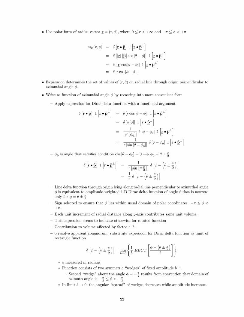
— Each unit increment of radial distance along y-axis contributes same unit volume.

— This expression seems to indicate otherwise for rotated function

— Contribution to volume affected by factor r−1.

— o resolve apparent conundrum, substitute expression for Dirac delta function as limit ofrectangle function

δhφ−

³θ ± π

2

´i= lim

b→0

(1

bRECT

"φ−

¡θ ± π

2

¢b

#)

∗ b measured in radians∗ Function consists of two symmetric “wedges” of fixed amplitude b−1.

· Second “wedge” about the angle φ = −π2 results from convention that domain of

azimuth angle is −π2 ≤ φ < +π

2 .

∗ In limit b→ 0, the angular “spread” of wedges decreases while amplitude increases.

22

∗ Contribution of segments of wedges with unit radial extent increases in proportionto radial distance r from origin.∗ Factor of r−1 compensates for increase in volume to ensure that contributions tovolume of segments with equal radial extent remain constant.

“Angular” delta function as limit of rectangle, limdφ→0

n1dφRECT

hφ−π

2

dφ

io.

• Other forms may be derived by manipulating argument

• Slope-intercept form of a line in the 2-D plane

δ£r • bp¤ 1 hr • bp⊥i = δ

∙+sin [φ]

µy +

x cos [φ]

sin [φ]

¶¸1 [x sin [φ]− y cos [φ]]

=

¯̄̄̄1

sin [φ]

¯̄̄̄δ [(y − (cot [−φ] x+ 0))] 1 [x sin [φ]− y cos [φ]]

• Dirac delta function evaluates to zero except at [x, y] that satisfy slope-intercept form ofstraight line

• y-intercept is zero

• Slope is s = cot [−φ] = − cot [φ]

23

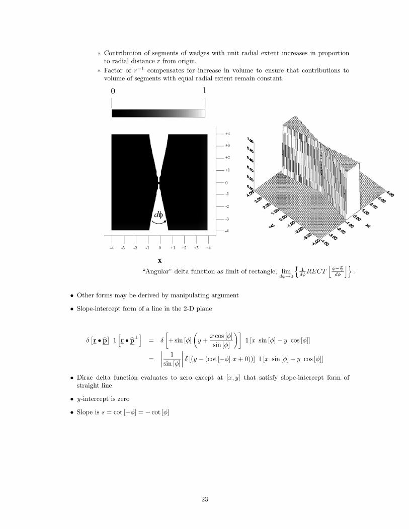
Two examples of rotated line delta functions as 1-D rectangle functions of width b. In both cases,the amplitude of the gray area is b−1. (a) The rectangle is a function of x with width b measuredon the x -axis and “perpendicular width” b cos (φ); (b) the rectangle is a function of y with

“perpendicular width” b sin [φ].

Three examples of line delta functions:

Different “flavors” of line delta functions: (a) δ£r · bp¤ 1 hr · bp⊥i through the origin perpendicular

to bp; (b) δ £p0 − r · bp¤ 1 hr · bp⊥i perpendicular to bp at a distance p0 < 0 from the origin; (c)

δhr · bp⊥i 1 £r · bp¤ through the origin parallel to bp.

24

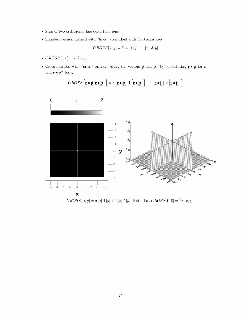
• Sum of two orthogonal line delta functions.

• Simplest version defined with “lines” coincident with Cartesian axes:

CROSS [x, y] = δ [x] 1 [y] + 1 [x] δ [y]

• CROSS [0, 0] = 2 δ [x, y]

• Cross function with “arms” oriented along the vectors bp and bp⊥ by substituting r • bp for xand r • bp⊥ for y :

CROSShr • bp, r • bp⊥i = δ

£r • bp¤ 1 hr • bp⊥i+ 1 £r • bp¤ δ hr • bp⊥i

CROSS [x, y] = δ [x] 1 [y] + 1 [x] δ [y]. Note that CROSS [0, 0] = 2 δ [x, y] .

25

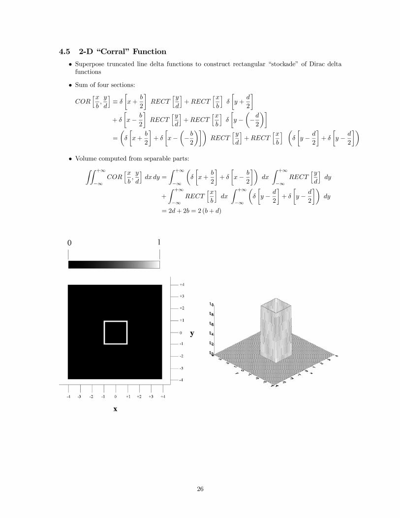
4.5 2-D “Corral” Function

• Superpose truncated line delta functions to construct rectangular “stockade” of Dirac deltafunctions

• Sum of four sections:

CORhxb,y

d

i≡ δ

∙x+

b

2

¸RECT

hyd

i+RECT

hxb

iδ

∙y +

d

2

¸+ δ

∙x− b

2

¸RECT

hyd

i+RECT

hxb

iδ

∙y −

µ−d2

¶¸=

µδ

∙x+

b

2

¸+ δ

∙x−

µ− b

2

¶¸¶RECT

hyd

i+RECT

hxb

i µδ

∙y − d

2

¸+ δ

∙y − d

2

¸¶• Volume computed from separable parts:ZZ +∞

−∞COR

hxb,y

d

idxdy =

Z +∞

−∞

µδ

∙x+

b

2

¸+ δ

∙x− b

2

¸¶dx

Z +∞

−∞RECT

hyd

idy

+

Z +∞

−∞RECT

hxb

idx

Z +∞

−∞

µδ

∙y − d

2

¸+ δ

∙y − d

2

¸¶dy

= 2d+ 2b = 2 (b+ d)

26

5 2-D Functions with Circular Symmetry• Vary along radial direction

• Constant in azimuthal direction

• All profiles along radial lines are identical

• Important in optics

• Optical systems are constructed from lenses with circular cross sections.

• Same amplitude at all points on circle of radius r0 centered at origin

• Amplitude of radial function fr (r0) replicated for [x, y] that satisfy x2 + y2 = r20.

• Circularly symmetric function expressed as orthogonal product of 1-D radial profile and unitconstant in azimuthal direction:

f [x, y] =⇒ f (r) = fr (r) 1 [θ] , 0 ≤ r < +∞, −π ≤ θ < +π

• Rotation about origin has no effect on amplitude

• Symmetric with respect to the origin

— Domains of radial and azimuthal variables may be recast wiht symmetric radial interval−∞ < r < +∞

— Azimuthal domain −π2 ≤ θ < +π

2 .

• Volume calculated in polar coordinates

• area element dx dy replaced by area element in polar coordinates r dr dθ:

ZZ +∞

−∞f [x, y] dx dy =

Z θ=+π

θ=−π

Z r=+∞

r=0

f (r) r dr

= 2π

Z +∞

0

fr (r) r dr

• Center of symmetry relocated to [x0, y0] by adding vector to argument:

f (r− r0) = f [x, y]

= f [|r| cos [θ]− |r0| cos [θ0] , |r|]

27

5.1 Cylinder (Circle) Function

• Unit amplitude inside radius r0

• Null amplitude outside

• Circularly symmetric version of 2-D rectangle

CY L

µr

d0

¶=

⎧⎪⎪⎪⎪⎨⎪⎪⎪⎪⎩1 for r < d0

2

12 for r = d0

2

0 for r < d02

• Area of enclosed circle of unit diameter is π4 ' 0.7854 <unit area of RECT [x, y].

• Volume of CY L³

rd0

´: Z +π

−πdθ

Z +∞

0

CY L

µr

d0

¶r d0r =

πd204

Example of 2-D cylinder function CY L¡r2

¢.

28

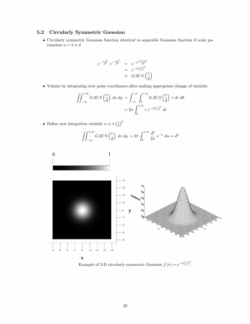
5.2 Circularly Symmetric Gaussian

• Circularly symmetric Gaussian function identical to separable Gaussian function if scale pa-rameters a = b ≡ d

e−πx2

d2 e−πy2

d2 = e−πx2+y2

d2

= e−π(rd )

2

≡ GAUS³rd

´• Volume by integrating over polar coordinates after making appropriate change of variable:ZZ +∞

−∞GAUS

³rd

´dx dy =

Z +π

−π

Z +∞

0

GAUS³rd

´r dr dθ

= 2π

Z +∞

0

r e−π(rd)

2

dr

• Define new integration variable α ≡ π¡rd

¢2ZZ +∞

−∞GAUS

³ rd

´dx dy = 2π

Z +∞

0

d2

2πe−α dα = d2

Example of 2-D circularly symmetric Gaussian f (r) = e−π(r2 )

2

.

29

5.3 Circularly Symmetric Bessel Function, Zero Order

J0 [2πrρ0] 1 [θ] = J0

³2πpx2 + y2 ρ0

´• Selectable parameter ρ0 analogous to spatial frequency of sinusoid

— Larger ρ0 =⇒shorter interval between successive maxima of Bessel function

• Appears in several imaging applications.

• J0 [2πrρ0] 1 [θ] generated by summing 2-D cosine functions with the same period “directed”along all azimuthal directions.

• Constituent functions have form cos [2π (ηx+ ηy)] , wherepξ2 + η2 = ρ20.

J0 [2πrρ0] 1 [θ] =

Z +π/2

−π/2cos [2π (ξx+ ηy)] dφ where ξ2 + η2 = ρ20

• Symmetry of integrand used to evaluate integral over domain of 2π radians:

J0 [2πrρ0] =1

2

Z +π

−πcos [2π (ξx+ ηy)] dφ, where ξ2 + η2 = ρ20

=1

2

Z +π

−πcos [2π (rξ cos [φ] + rη sin [φ])] dφ

• Rewrite integrals by substituting corresponding linear-phase complex exponential for cosinefunction

J0 [2πrρ0] 1 [θ] =1

π

Z +π/2

−π/2e±2πi(ξx+ηy)dφ

=1

2π

Z +π

−πe±2πi(ξx+ηy) dφ

=1

2π

Z +π

−πcos [2πr (ξ cos [φ] + η sin [φ])] dφ, where ξ2 + η2 = ρ20

• Profile along the x-axis by setting η = 0. Spatial frequency ξ along x-axis becomes ξ = ρ0:

J0 [2πrρ0] 1 [θ]|η=0 = J0 [2πxρ0]

=1

π

Z +π/2

−π/2cos [2πrρ0 cos [φ]] dφ

=1

2π

Z +π

−πcos [2πrρ0 cos [φ]] dφ

= J0 [2πxξ]|r=x,ξ=ρ0 = J0 [2πrρ0]

• ρ0 cos [φ] is spatial frequency of constituent 1-D cosines of Bessel function

— Suggests alternate interpretation that 1-D J0 Bessel function is sum of 1-D cosines withspatial frequencies in interval −ρ0 ≤ ξ ≤ +ρ0 but weighted in “density” by cos [φ]

— Largest spatial frequency exists when φ = 0, while the cosine is the unit constant whenφ = ±π

2 .

30

• Equivalent expressions for 1-D Bessel function obtained by setting ξ = 0 so that η = ρ0

— equivalent to projecting argument onto y-axis:

J0 [2πyη] 1 [θ]|ξ=0 =1

π

Z +π/2

−π/2cos [2πr (ρ0 sin [φ])] dφ

=1

2π

Z +π2

0

cos [2πr (ρ0 sin [φ])] dφ

= J0 [2πyη]|r=y,η=ρ0 = J0 [2πrρ0]

— Projection of complex-valued formulations onto x-axis is:

(J0 [2πyρ0] 1 [θ])|ξ=0 =1

π

Z +π/2

−π/2e±2πirρ0 cos[φ] dφ where ξ2 + η2 = ρ20

— May be used as an equivalent definition of the Bessel function.

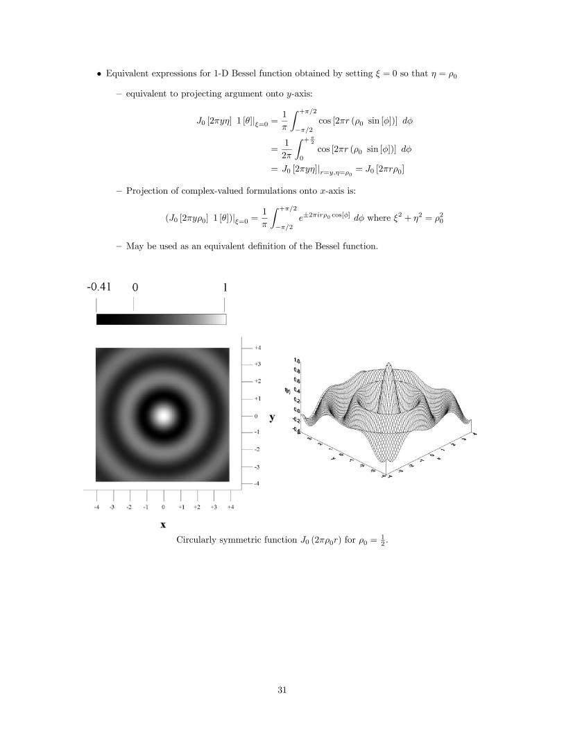
Circularly symmetric function J0 (2πρ0r) for ρ0 =12 .

31

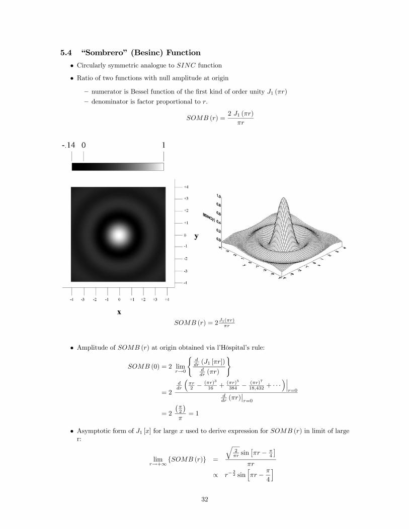
5.4 “Sombrero” (Besinc) Function

• Circularly symmetric analogue to SINC function

• Ratio of two functions with null amplitude at origin

— numerator is Bessel function of the first kind of order unity J1 (πr)— denominator is factor proportional to r.

SOMB (r) =2 J1 (πr)

πr

SOMB (r) = 2J1(πr)πr

• Amplitude of SOMB (r) at origin obtained via l’Hôspital’s rule:

SOMB (0) = 2 limr→0

(ddr (J1 [πr])

ddr (πr)

)

= 2

ddr

³πr2 −

(πr)3

16 + (πr)5

384 −(πr)7

18,432 + · · ·´¯̄̄

r=0ddr (πr)

¯̄r=0

= 2

¡π2

¢π

= 1

• Asymptotic form of J1 [x] for large x used to derive expression for SOMB (r) in limit of larger:

limr→+∞

{SOMB (r)} =

q2πr sin

£πr − π

4

¤πr

∝ r−32 sin

hπr − π

4

i

32

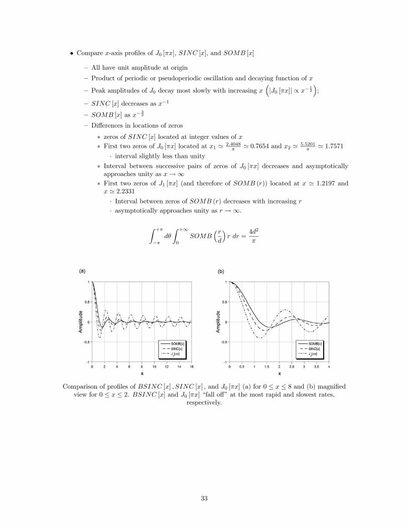
• Compare x-axis profiles of J0 [πx], SINC [x], and SOMB [x]

— All have unit amplitude at origin

— Product of periodic or pseudoperiodic oscillation and decaying function of x

— Peak amplitudes of J0 decay most slowly with increasing x³|J0 [πx]| ∝ x−

12

´;

— SINC [x] decreases as x−1

— SOMB [x] as x−32

— Differences in locations of zeros

∗ zeros of SINC [x] located at integer values of x∗ First two zeros of J0 [πx] located at x1 ' 2.4048

π ' 0.7654 and x2 ' 5.5201π ' 1.7571

· interval slightly less than unity∗ Interval between successive pairs of zeros of J0 [πx] decreases and asymptoticallyapproaches unity as x→∞∗ First two zeros of J1 [πx] (and therefore of SOMB (r)) located at x ' 1.2197 andx ' 2.2331· Interval between zeros of SOMB (r) decreases with increasing r· asymptotically approaches unity as r→∞.

Z +π

−πdθ

Z +∞

0

SOMB³ rd

´r dr =

4d2

π

Comparison of profiles of BSINC [x] , SINC [x] , and J0 [πx] (a) for 0 ≤ x ≤ 8 and (b) magnifiedview for 0 ≤ x ≤ 2. BSINC [x] and J0 [πx] “fall off” at the most rapid and slowest rates,

respectively.

33

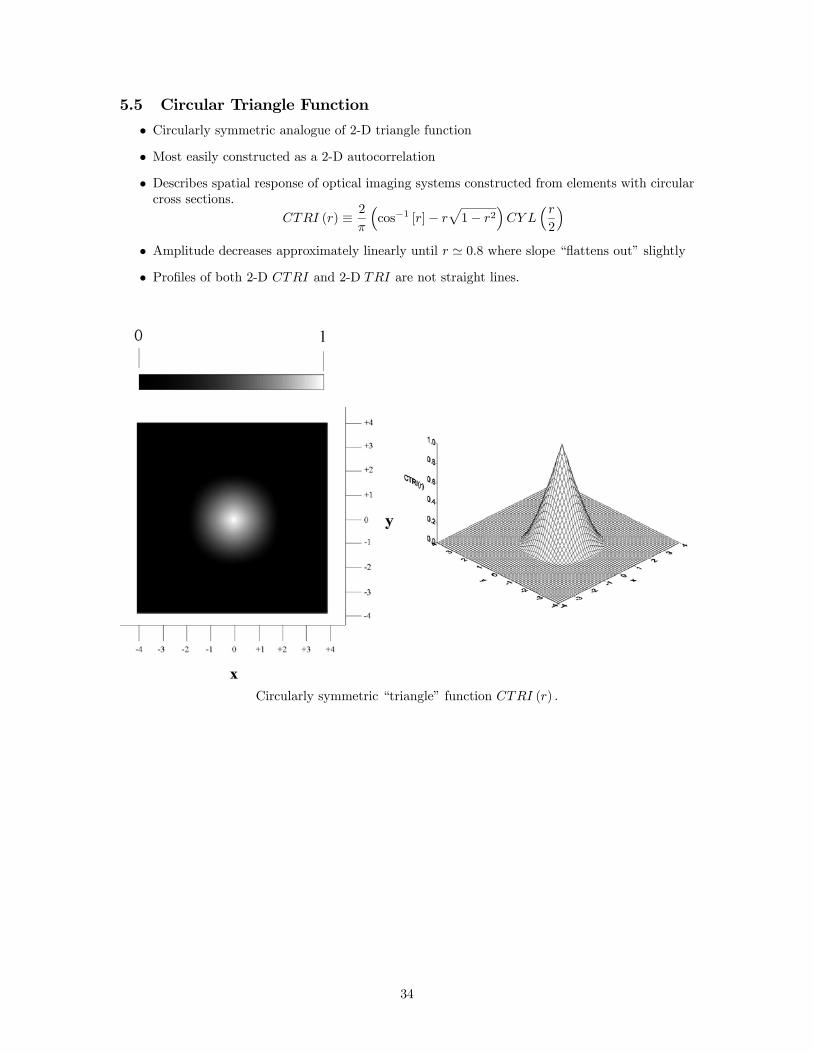
5.5 Circular Triangle Function

• Circularly symmetric analogue of 2-D triangle function

• Most easily constructed as a 2-D autocorrelation

• Describes spatial response of optical imaging systems constructed from elements with circularcross sections.

CTRI (r) ≡ 2

π

³cos−1 [r]− r

p1− r2

´CY L

³r2

´• Amplitude decreases approximately linearly until r ' 0.8 where slope “flattens out” slightly

• Profiles of both 2-D CTRI and 2-D TRI are not straight lines.

Circularly symmetric “triangle” function CTRI (r) .

34

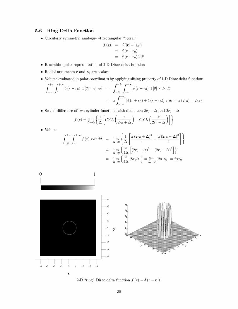
5.6 Ring Delta Function

• Circularly symmetric analogue of rectangular “corral”:f (r) = δ (|r|− |r0|)

≡ δ (r − r0)

= δ (r − r0) 1 [θ]

• Resembles polar representation of 2-D Dirac delta function

• Radial arguments r and r0 are scalars

• Volume evaluated in polar coordinates by applying sifting property of 1-D Dirac delta function:Z +π

−π

Z +∞

0

δ (r − r0) 1 [θ] r dr dθ =

Z +π2

−π2

Z +∞

−∞δ (r − r0) 1 [θ] r dr dθ

= π

Z +∞

−∞[δ (r + r0) + δ (r − r0)] r dr = π (2r0) = 2πr0

• Scaled difference of two cylinder functions with diameters 2r0 +∆ and 2r0 −∆:

f (r) = lim∆→0

½1

∆

∙CY L

µr

2r0 +∆

¶− CY L

µr

2r0 −∆

¶¸¾• Volume: Z +π

−π

Z +∞

0

f (r) r dr dθ = lim∆→0

(1

∆

"π (2r0 +∆)

2

4− π (2r0 −∆)2

4

#)= lim

∆→0

n π

4∆

h(2r0 +∆)

2 − (2r0 −∆)2io

= lim∆→0

n π

4∆[8r0∆]

o= lim∆→0

{2π r0} = 2πr0

2-D “ring” Dirac delta function f (r) = δ (r − r0) .

35

6 Complex-Valued 2-D Functions

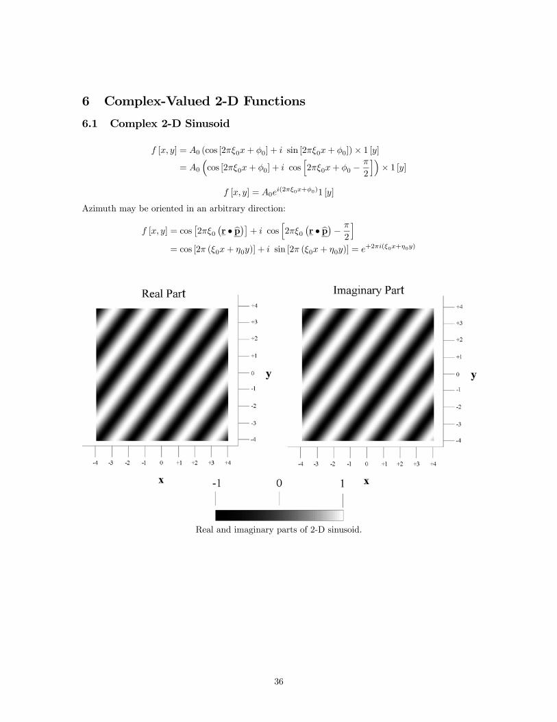
6.1 Complex 2-D Sinusoid

f [x, y] = A0 (cos [2πξ0x+ φ0] + i sin [2πξ0x+ φ0])× 1 [y]

= A0

³cos [2πξ0x+ φ0] + i cos

h2πξ0x+ φ0 −

π

2

i´× 1 [y]

f [x, y] = A0ei(2πξ0x+φ0)1 [y]

Azimuth may be oriented in an arbitrary direction:

f [x, y] = cos£2πξ0

¡r • bp¢¤+ i cos

h2πξ0

¡r • bp¢− π

2

i= cos [2π (ξ0x+ η0y)] + i sin [2π (ξ0x+ η0y)] = e+2πi(ξ0x+η0y)

Real and imaginary parts of 2-D sinusoid.

36

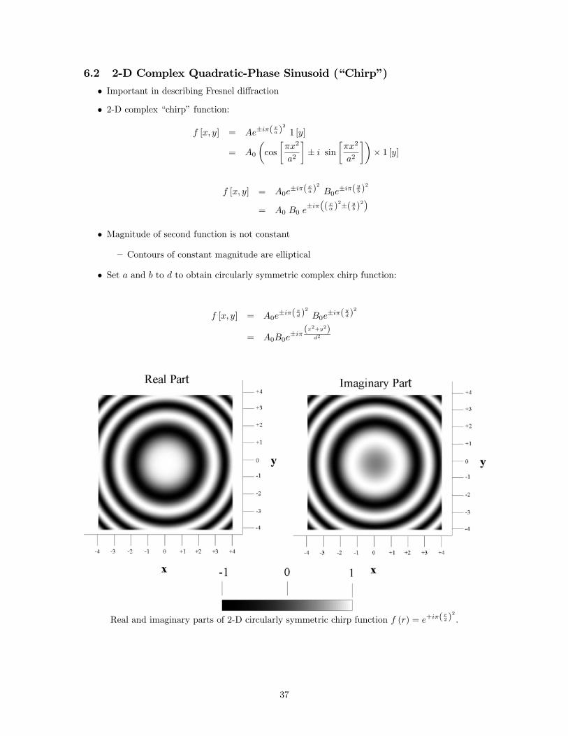
6.2 2-D Complex Quadratic-Phase Sinusoid (“Chirp”)

• Important in describing Fresnel diffraction

• 2-D complex “chirp” function:

f [x, y] = Ae±iπ(xa )

2

1 [y]

= A0

µcos

∙πx2

a2

¸± i sin

∙πx2

a2

¸¶× 1 [y]

f [x, y] = A0e±iπ(xa )

2

B0e±iπ( yb )

2

= A0 B0 e±iπ ( xα)

2±( yb )2

• Magnitude of second function is not constant

— Contours of constant magnitude are elliptical

• Set a and b to d to obtain circularly symmetric complex chirp function:

f [x, y] = A0e±iπ( xd )

2

B0e±iπ( yd )

2

= A0B0e±iπ (

x2+y2)d2

Real and imaginary parts of 2-D circularly symmetric chirp function f (r) = e+iπ(r2 )

2

.

37