Embed Size (px)
Citation preview

1 1 Slide
Slide
© 2008 Thomson South-Western. All Rights Reserved© 2008 Thomson South-Western. All Rights Reserved
DSCI 3870 Chapter 5
ADVANCED LP APPLICATIONS
Additional Reading Material

2 2 Slide
Slide
© 2008 Thomson South-Western. All Rights Reserved© 2008 Thomson South-Western. All Rights Reserved
Chapter 5 – Advanced LP ApplicationsChapter 5 – Advanced LP Applications Additional Reading Material Additional Reading Material
Revenue ManagementRevenue Management Portfolio Models and Asset AllocationPortfolio Models and Asset Allocation Game Theory – Part IIGame Theory – Part II

3 3 Slide
Slide
© 2008 Thomson South-Western. All Rights Reserved© 2008 Thomson South-Western. All Rights Reserved
Revenue ManagementRevenue Management
Another LP application is revenue Another LP application is revenue management.management.
Revenue managementRevenue management involves managing the involves managing the short-term demand for a fixed perishable short-term demand for a fixed perishable inventory in order to maximize revenue inventory in order to maximize revenue potential.potential.
The methodology was first used to determine The methodology was first used to determine how many airline seats to sell at an early-how many airline seats to sell at an early-reservation discount fare and many to sell at a reservation discount fare and many to sell at a full fare.full fare.
Application areas now include hotels, Application areas now include hotels, apartment rentals, car rentals, cruise lines, apartment rentals, car rentals, cruise lines, and golf courses.and golf courses.

4 4 Slide
Slide
© 2008 Thomson South-Western. All Rights Reserved© 2008 Thomson South-Western. All Rights Reserved
Revenue ManagementRevenue Management
LeapFrog Airways provides passenger service LeapFrog Airways provides passenger service forforIndianapolis, Baltimore, Memphis, Austin, and Indianapolis, Baltimore, Memphis, Austin, and Tampa.Tampa.LeapFrog has two WB828 airplanes,LeapFrog has two WB828 airplanes,one based in Indianapolis and theone based in Indianapolis and theother in Baltimore. Each morningother in Baltimore. Each morningthe Indianapolis based plane flies tothe Indianapolis based plane flies toAustin with a stopover in Memphis.Austin with a stopover in Memphis.The Baltimore based plane flies toThe Baltimore based plane flies toTampa with a stopover in Memphis.Tampa with a stopover in Memphis.Both planes have a coach section with a 120-seat Both planes have a coach section with a 120-seat capacity. capacity.
5 5 Slide
Slide
© 2008 Thomson South-Western. All Rights Reserved© 2008 Thomson South-Western. All Rights Reserved
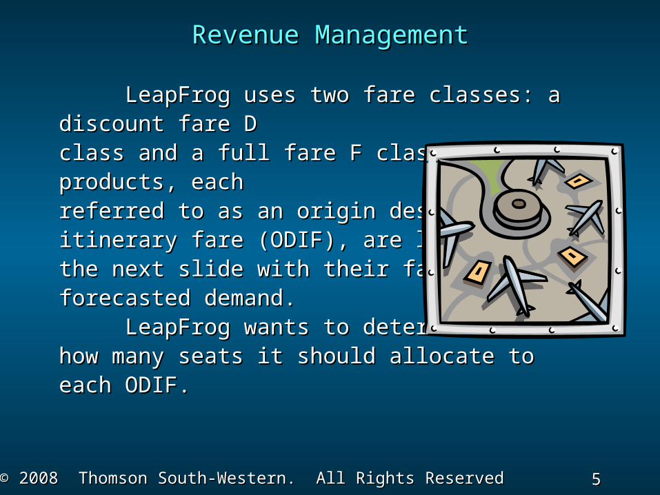
LeapFrog uses two fare classes: a discount fare LeapFrog uses two fare classes: a discount fare DDclass and a full fare F class. Leapfrog’s products, class and a full fare F class. Leapfrog’s products, eacheachreferred to as an origin destinationreferred to as an origin destinationitinerary fare (ODIF), are listed onitinerary fare (ODIF), are listed onthe next slide with their fares andthe next slide with their fares andforecasted demand.forecasted demand. LeapFrog wants to determineLeapFrog wants to determinehow many seats it should allocate tohow many seats it should allocate toeach ODIF.each ODIF.
Revenue ManagementRevenue Management

6 6 Slide
Slide
© 2008 Thomson South-Western. All Rights Reserved© 2008 Thomson South-Western. All Rights Reserved
Revenue ManagementRevenue Management

7 7 Slide
Slide
© 2008 Thomson South-Western. All Rights Reserved© 2008 Thomson South-Western. All Rights Reserved
Revenue ManagementRevenue Management
Define the Decision VariablesDefine the Decision Variables
There are 16 variables, one for each ODIF:There are 16 variables, one for each ODIF:
IMD = number of seats allocated to Indianapolis-IMD = number of seats allocated to Indianapolis-Memphis-Memphis-
Discount classDiscount classIAD = number of seats allocated to Indianapolis-IAD = number of seats allocated to Indianapolis-Austin-Austin- Discount classDiscount classITD = number of seats allocated to Indianapolis-ITD = number of seats allocated to Indianapolis-Tampa-Tampa- Discount classDiscount classIMF = number of seats allocated to Indianapolis-IMF = number of seats allocated to Indianapolis-Memphis-Memphis- Full Fare classFull Fare classIAF = number of seats allocated to Indianapolis-IAF = number of seats allocated to Indianapolis-Austin-Full Austin-Full Fare classFare class

8 8 Slide
Slide
© 2008 Thomson South-Western. All Rights Reserved© 2008 Thomson South-Western. All Rights Reserved
Revenue ManagementRevenue Management
Define the Decision Variables (continued)Define the Decision Variables (continued)
ITF = number of seats allocated to Indianapolis-ITF = number of seats allocated to Indianapolis-Tampa-Tampa- Full Fare classFull Fare classBMD = number of seats allocated to Baltimore-BMD = number of seats allocated to Baltimore-Memphis-Memphis- Discount classDiscount classBAD = number of seats allocated to Baltimore-BAD = number of seats allocated to Baltimore-Austin-Austin- Discount classDiscount classBTD = number of seats allocated to Baltimore-BTD = number of seats allocated to Baltimore-Tampa-Tampa- Discount classDiscount classBMF = number of seats allocated to Baltimore-BMF = number of seats allocated to Baltimore-Memphis-Memphis- Full Fare classFull Fare classBAF = number of seats allocated to Baltimore-BAF = number of seats allocated to Baltimore-Austin-Austin- Full Fare classFull Fare class

9 9 Slide
Slide
© 2008 Thomson South-Western. All Rights Reserved© 2008 Thomson South-Western. All Rights Reserved
Revenue ManagementRevenue Management
Define the Decision Variables (continued)Define the Decision Variables (continued)
BTF = number of seats allocated to Baltimore-BTF = number of seats allocated to Baltimore-Tampa-Tampa- Full Fare classFull Fare classMAD = number of seats allocated to Memphis-MAD = number of seats allocated to Memphis-Austin-Austin- Discount classDiscount classMTD = number of seats allocated to Memphis-MTD = number of seats allocated to Memphis-Tampa-Tampa- Discount classDiscount classMAF = number of seats allocated to Memphis-MAF = number of seats allocated to Memphis-Austin-Austin- Full Fare classFull Fare classMTF = number of seats allocated to Memphis-MTF = number of seats allocated to Memphis-Tampa-Tampa- Full Fare classFull Fare class

10 10 Slide
Slide
© 2008 Thomson South-Western. All Rights Reserved© 2008 Thomson South-Western. All Rights Reserved
Revenue ManagementRevenue Management
Define the Objective FunctionDefine the Objective Function
Maximize total revenue:Maximize total revenue:
Max (fare per seat for each ODIF)Max (fare per seat for each ODIF)
x (number of seats allocated to the x (number of seats allocated to the ODIF)ODIF)
Max 175IMD + 275IAD + 285ITD + 395IMFMax 175IMD + 275IAD + 285ITD + 395IMF
+ 425IAF + 475ITF + 185BMD + 315BAD+ 425IAF + 475ITF + 185BMD + 315BAD
+ 290BTD + 385BMF + 525BAF + + 290BTD + 385BMF + 525BAF + 490BTF490BTF
+ 190MAD + 180MTD + 310MAF + + 190MAD + 180MTD + 310MAF + 295MTF295MTF

11 11 Slide
Slide
© 2008 Thomson South-Western. All Rights Reserved© 2008 Thomson South-Western. All Rights Reserved
Revenue ManagementRevenue Management
Define the ConstraintsDefine the Constraints
There are 4 capacity constraints, one for each There are 4 capacity constraints, one for each flight leg:flight leg:
Indianapolis-Memphis legIndianapolis-Memphis leg
(1)(1) IMD + IAD + ITD + IMF + IAF + ITF IMD + IAD + ITD + IMF + IAF + ITF << 120 120
Baltimore-Memphis legBaltimore-Memphis leg
(2)(2) BMD + BAD + BTD + BMF + BAF + BTF BMD + BAD + BTD + BMF + BAF + BTF << 120 120
Memphis-Austin legMemphis-Austin leg
(3)(3) IAD + IAF + BAD + BAF + MAD + MAF IAD + IAF + BAD + BAF + MAD + MAF << 120 120
Memphis-Tampa legMemphis-Tampa leg
(4)(4) ITD + ITF + BTD + BTF + MTD + MTF ITD + ITF + BTD + BTF + MTD + MTF << 120120

12 12 Slide
Slide
© 2008 Thomson South-Western. All Rights Reserved© 2008 Thomson South-Western. All Rights Reserved
Revenue ManagementRevenue Management
Define the Constraints (continued)Define the Constraints (continued)
There are 16 demand constraints, one for each There are 16 demand constraints, one for each ODIF:ODIF:
(5) IMD (5) IMD << 44 44 (11) BMD (11) BMD << 26 26 (17) MAD (17) MAD << 55
(6) IAD (6) IAD << 25 25 (12) BAD (12) BAD << 50 50 (18) MTD (18) MTD << 4848
(7) ITD (7) ITD << 40 40 (13) BTD (13) BTD << 42 42 (19) MAF (19) MAF << 1414
(8) IMF (8) IMF << 15 15 (14) BMF (14) BMF << 12 12 (20) MTF (20) MTF << 1111
(9) IAF (9) IAF << 10 10 (15) BAF (15) BAF << 16 16
(10) ITF (10) ITF << 8 8 (16) BTF (16) BTF << 9 9

13 13 Slide
Slide
© 2008 Thomson South-Western. All Rights Reserved© 2008 Thomson South-Western. All Rights Reserved
Revenue ManagementRevenue Management
The Management ScientistThe Management Scientist Solution Solution
Objective Function Value = 94735.000Objective Function Value = 94735.000
VariableVariable ValueValue Reduced Reduced CostCost
IMDIMD 44.000 0.00044.000 0.000 IADIAD 3.000 0.000 3.000 0.000 ITD ITD 40.000 40.000
0.0000.000 IMF IMF 15.000 15.000
0.0000.000 IAF IAF 10.000 10.000
0.0000.000 ITF ITF 8.000 8.000
0.0000.000 BMD BMD 26.000 26.000
0.0000.000 BAD BAD 50.000 50.000
0.0000.000

14 14 Slide
Slide
© 2008 Thomson South-Western. All Rights Reserved© 2008 Thomson South-Western. All Rights Reserved
Revenue ManagementRevenue Management
The Management ScientistThe Management Scientist Solution Solution (continued)(continued)
VariableVariable ValueValue Reduced CostReduced Cost
BTD BTD 7.000 7.000 0.000 0.000
BMF BMF 12.000 12.000 0.000 0.000
BAF BAF 16.000 16.000 0.000 0.000
BTF BTF 9.000 9.000 0.000 0.000
MAD MAD 27.000 27.000 0.000 0.000
MTD MTD 45.000 45.000 0.000 0.000
MAF MAF 14.000 14.000 0.000 0.000
MTF MTF 11.000 11.000 0.000 0.000
15 15 Slide
Slide
© 2008 Thomson South-Western. All Rights Reserved© 2008 Thomson South-Western. All Rights Reserved
Portfolio Models and Asset ManagementPortfolio Models and Asset Management
Asset allocationAsset allocation involves determining how to involves determining how to allocate investment funds across a variety of allocate investment funds across a variety of asset classes such as stocks, bonds, mutual asset classes such as stocks, bonds, mutual funds, real estate. funds, real estate.
Portfolio modelsPortfolio models are used to determine are used to determine percentage of funds that should be made in percentage of funds that should be made in each asset class.each asset class.
The goal is to create a portfolio that provides The goal is to create a portfolio that provides the best balance between risk and return.the best balance between risk and return.

16 16 Slide
Slide
© 2008 Thomson South-Western. All Rights Reserved© 2008 Thomson South-Western. All Rights Reserved
John Sweeney is an investment advisor who John Sweeney is an investment advisor who isisattempting to construct an "optimal portfolio" attempting to construct an "optimal portfolio" for afor aclient who has $400,000 cash to invest. There client who has $400,000 cash to invest. There are tenare tendifferent investments, falling into fourdifferent investments, falling into fourbroad categories that John and his clientbroad categories that John and his clienthave identified as potential candidatehave identified as potential candidatefor this portfolio.for this portfolio. The investments and their importantThe investments and their importantcharacteristics are listed in the table oncharacteristics are listed in the table onthe next slide. Note that Unidyde Corp.the next slide. Note that Unidyde Corp.Corp. under Equities and Unidyde Corp. under Corp. under Equities and Unidyde Corp. under Debt Debt are two separate investments, whereas First are two separate investments, whereas First General General REIT is a single investment that is considered REIT is a single investment that is considered both anboth anequities and a real estate investment.equities and a real estate investment.
Portfolio ModelPortfolio Model

17 17 Slide
Slide
© 2008 Thomson South-Western. All Rights Reserved© 2008 Thomson South-Western. All Rights Reserved
Portfolio ModelPortfolio Model
Exp. AnnualExp. Annual After Tax Liquidity After Tax Liquidity RiskRiskCategory Category Investment Investment Return Factor Return Factor FactorFactor
Equities Equities Unidyde Corp. Unidyde Corp. 15.0% 100 15.0% 100 6060(Stocks)(Stocks) CC’s Restaurants CC’s Restaurants 17.0% 100 17.0% 100 70 70 First General REIT First General REIT 17.5% 100 17.5% 100 75 75
Debt Debt Metropolis Electric Metropolis Electric 11.8% 95 11.8% 95 20 20(Bonds) (Bonds) Unidyde Corp. Unidyde Corp. 12.2% 92 12.2% 92 30 30 Lewisville Transit Lewisville Transit 12.0% 79 12.0% 79 22 22
Real Estate Real Estate Realty PartnersRealty Partners 22.0% 0 22.0% 0 50 50 First General REIT First General REIT ( --- See ( --- See above --- )above --- )
Money Money T-Bill Account T-Bill Account 9.6% 80 9.6% 80 0 0 Money Mkt. Fund Money Mkt. Fund 10.5% 100 10.5% 100 1010 Saver's Certificate Saver's Certificate 12.6% 0 12.6% 0 0 0

18 18 Slide
Slide
© 2008 Thomson South-Western. All Rights Reserved© 2008 Thomson South-Western. All Rights Reserved
Portfolio ModelPortfolio Model
Formulate a linear programming problem toFormulate a linear programming problem toaccomplish John's objective as an investment accomplish John's objective as an investment advisor advisor which is to construct a portfolio that maximizes which is to construct a portfolio that maximizes hishisclient's total expected after-tax return over the client's total expected after-tax return over the next year, subject to the limitations placed upon next year, subject to the limitations placed upon him by the client for the portfolio. (Limitations him by the client for the portfolio. (Limitations listed on next two slides.)listed on next two slides.)

19 19 Slide
Slide
© 2008 Thomson South-Western. All Rights Reserved© 2008 Thomson South-Western. All Rights Reserved
Portfolio ModelPortfolio Model
Portfolio LimitationsPortfolio Limitations
1. The weighted average liquidity factor for the portfolio1. The weighted average liquidity factor for the portfolio must to be at least 65.must to be at least 65.
2. The weighted average risk factor for the portfolio must2. The weighted average risk factor for the portfolio must be no greater than 55.be no greater than 55.
3. No more than $60,000 is to be invested in Unidyde3. No more than $60,000 is to be invested in Unidyde stocks or bonds.stocks or bonds.
4. No more than 40% of the investment can be in any one4. No more than 40% of the investment can be in any one category except the money category.category except the money category.
5. No more than 20% of the total investment can be in5. No more than 20% of the total investment can be in any one investment except the money market fund.any one investment except the money market fund.
continuedcontinued

20 20 Slide
Slide
© 2008 Thomson South-Western. All Rights Reserved© 2008 Thomson South-Western. All Rights Reserved
Portfolio ModelPortfolio Model
Portfolio Limitations (continued) Portfolio Limitations (continued)
6. At least $1,000 must be invested in the Money Market6. At least $1,000 must be invested in the Money Market fund.fund.
7. The maximum investment in Saver's Certificates is7. The maximum investment in Saver's Certificates is $15,000.$15,000.
8. The minimum investment desired for debt is $90,000.8. The minimum investment desired for debt is $90,000.
9. At least $10,000 must be placed in a T-Bill account.9. At least $10,000 must be placed in a T-Bill account.

21 21 Slide
Slide
© 2008 Thomson South-Western. All Rights Reserved© 2008 Thomson South-Western. All Rights Reserved
Portfolio ModelPortfolio Model
Define the Decision VariablesDefine the Decision Variables
X1 = $ amount invested in X1 = $ amount invested in Unidyde Corp. Unidyde Corp. (Equities)(Equities)
X2 = $ amount invested in CC’s RestaurantsX2 = $ amount invested in CC’s Restaurants
X3 = $ amount invested in First General REITX3 = $ amount invested in First General REIT
X4 = $ amount invested in Metropolis ElectricX4 = $ amount invested in Metropolis Electric
X5 = $ amount invested in Unidyde Corp. X5 = $ amount invested in Unidyde Corp. (Debt) (Debt)
X6 = $ amount invested in Lewisville TransitX6 = $ amount invested in Lewisville Transit
X7 = $ amount invested in Realty PartnersX7 = $ amount invested in Realty Partners
X8 = $ amount invested in T-Bill Account X8 = $ amount invested in T-Bill Account
X9 = $ amount invested in Money Mkt. FundX9 = $ amount invested in Money Mkt. Fund
X10 = $ amount invested in Saver's Certificate X10 = $ amount invested in Saver's Certificate

22 22 Slide
Slide
© 2008 Thomson South-Western. All Rights Reserved© 2008 Thomson South-Western. All Rights Reserved
Portfolio ModelPortfolio Model
Define the Objective FunctionDefine the Objective Function
Maximize the Maximize the total expected after-tax return total expected after-tax return over the next yearover the next year::
Max .15X1 + .17Max .15X1 + .17X2 + .175X3 + .118X4 X2 + .175X3 + .118X4 + .122X5+ .122X5
+ .12X6 + .22X7 + .096X8 + .105X9 + .12X6 + .22X7 + .096X8 + .105X9 + .126X10 + .126X10
23 23 Slide
Slide
© 2008 Thomson South-Western. All Rights Reserved© 2008 Thomson South-Western. All Rights Reserved
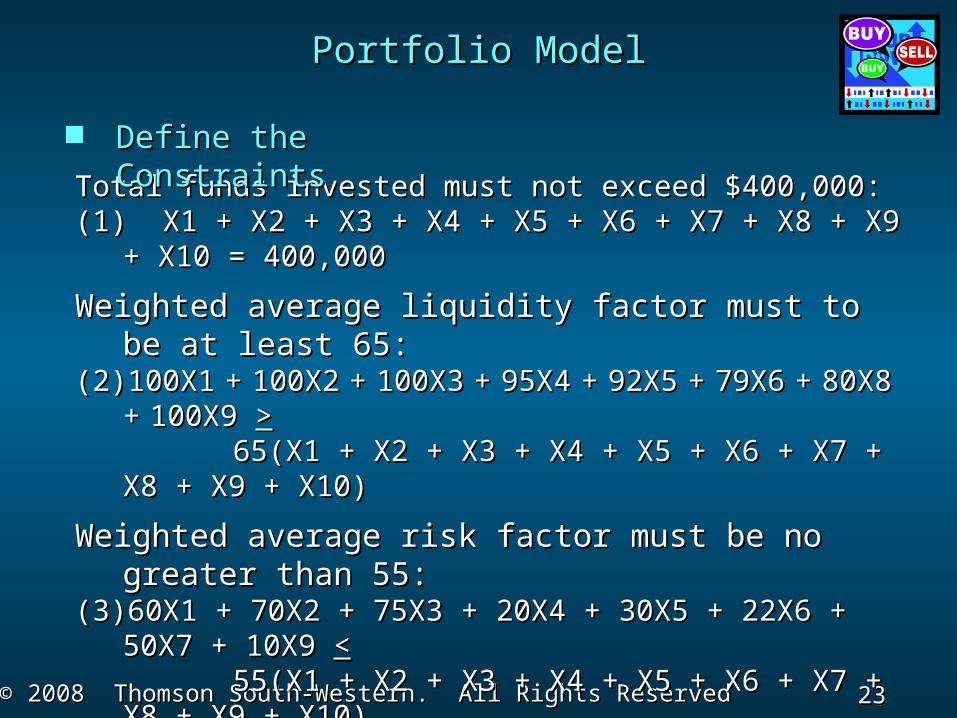
Portfolio ModelPortfolio Model
Total funds invested must not exceed $400,000:Total funds invested must not exceed $400,000:(1) X1 + X2 + X3 + X4 + X5 + X6 + X7 + X8 + X9 + (1) X1 + X2 + X3 + X4 + X5 + X6 + X7 + X8 + X9 +
X10 = 400,000X10 = 400,000
Weighted average liquidity factor must to be at Weighted average liquidity factor must to be at least 65:least 65:
(2)(2) 100X1100X1 ++ 100X2100X2 ++ 100X3100X3 ++ 95X495X4 ++ 92X592X5 ++ 79X679X6 ++
80X880X8 ++ 100X9 100X9 >> 65(X1 + X2 + X3 + X4 + X5 + X6 + X7 + X8 + X9 65(X1 + X2 + X3 + X4 + X5 + X6 + X7 + X8 + X9
+ X10)+ X10)
Weighted average risk factor must be no greater Weighted average risk factor must be no greater than 55:than 55:
(3)(3) 60X1 + 70X2 + 75X3 + 20X4 + 30X5 + 22X6 + 50X7 60X1 + 70X2 + 75X3 + 20X4 + 30X5 + 22X6 + 50X7 + 10X9 + 10X9 <<
55(X1 + X2 + X3 + X4 + X5 + X6 + X7 + X8 + X9 55(X1 + X2 + X3 + X4 + X5 + X6 + X7 + X8 + X9 + X10)+ X10)
No more than $60,000 to be invested in Unidyde No more than $60,000 to be invested in Unidyde Corp:Corp:
(4)(4) X1 + X5 X1 + X5 << 60,000 60,000
Define the Define the ConstraintsConstraints

24 24 Slide
Slide
© 2008 Thomson South-Western. All Rights Reserved© 2008 Thomson South-Western. All Rights Reserved
Portfolio ModelPortfolio Model
Define the Constraints Define the Constraints (continued)(continued)No more than 40% of the $400,000 investment No more than 40% of the $400,000 investment can becan be
in any one category except the money category:in any one category except the money category:(5) X1 + X2 + X3 (5) X1 + X2 + X3 << 160,000 160,000(6) X4 + X5 + X6 (6) X4 + X5 + X6 << 160,000 160,000(7)(7) X3 + X7 X3 + X7 << 160,000 160,000
No more than 20% of the $400,000 investment No more than 20% of the $400,000 investment can becan be
in any one investment except the money market in any one investment except the money market fund:fund:
(8) X2 (8) X2 << 80,000 80,000 (12) X7 (12) X7 << 80,000 80,000(9) X3 (9) X3 << 80,000 80,000 (13) X8 (13) X8 << 80,000 80,000(10) X4 (10) X4 << 80,000 80,000 (14) X10 (14) X10 << 80,000 80,000(11) X6 (11) X6 << 80,000 80,000

25 25 Slide
Slide
© 2008 Thomson South-Western. All Rights Reserved© 2008 Thomson South-Western. All Rights Reserved
Portfolio ModelPortfolio Model
Define the Constraints Define the Constraints (continued)(continued)At least $1,000 must be invested in the Money At least $1,000 must be invested in the Money Market fund:Market fund:
(15) X9 (15) X9 >> 1,000 1,000
The maximum investment in Saver's Certificates is The maximum investment in Saver's Certificates is $15,000:$15,000:
(16) X10 (16) X10 << 15,000 15,000
The minimum investment the Debt category is The minimum investment the Debt category is $90,000:$90,000:
(17) X4 + X5 + X6 (17) X4 + X5 + X6 >> 90,000 90,000
At least $10,000 must be placed in a T-Bill account:At least $10,000 must be placed in a T-Bill account:(18) X8 (18) X8 >> 10,000 10,000
Non-negativity of variables:Non-negativity of variables: Xj Xj >> 0 j = 1, . . . , 10 0 j = 1, . . . , 10

26 26 Slide
Slide
© 2008 Thomson South-Western. All Rights Reserved© 2008 Thomson South-Western. All Rights Reserved
Portfolio ModelPortfolio Model
Solution SummarySolution Summary
Total Expected After-Tax Return = $64,355Total Expected After-Tax Return = $64,355X1 = $0 X1 = $0 invested in invested in Unidyde Corp. Unidyde Corp. (Equities)(Equities)X2 = $80,000 invested in CC’s RestaurantsX2 = $80,000 invested in CC’s RestaurantsX3 = $80,000 invested in First General REITX3 = $80,000 invested in First General REITX4 = $0X4 = $0 invested in Metropolis Electric invested in Metropolis ElectricX5 = $60,000 invested in Unidyde Corp. (Debt) X5 = $60,000 invested in Unidyde Corp. (Debt) X6 = $74,000 invested in Lewisville TransitX6 = $74,000 invested in Lewisville TransitX7 = $80,000 invested in Realty PartnersX7 = $80,000 invested in Realty PartnersX8 = $10,000 invested in T-Bill Account X8 = $10,000 invested in T-Bill Account X9 = $1,000 invested in Money Mkt. FundX9 = $1,000 invested in Money Mkt. Fund
X10 = $15,000 invested in Saver's Certificate X10 = $15,000 invested in Saver's Certificate

27 27 Slide
Slide
© 2008 Thomson South-Western. All Rights Reserved© 2008 Thomson South-Western. All Rights Reserved
Zero-Sum Games: Dominated Strategies Zero-Sum Games: Dominated Strategies ExampleExample
RowRowMinimumMinimum
-2-2
00
-3-3
bb11 bb33bb22
Player BPlayer B
1 0 1 0 3 3 3 4 3 4 -3 -3
aa11
aa22
aa33
Player APlayer A
ColumnColumnMaximumMaximum 6 5 6 5
3 3
6 5 6 5 -2 -2
Suppose that the payoff table for a two-person Suppose that the payoff table for a two-person zero-zero-sum game is the following. Here there is no sum game is the following. Here there is no optimaloptimalpure strategy.pure strategy.
MaximinMaximin
MinimaxMinimax

28 28 Slide
Slide
© 2008 Thomson South-Western. All Rights Reserved© 2008 Thomson South-Western. All Rights Reserved
Dominated Strategies ExampleDominated Strategies Example
bb11 bb33bb22
Player BPlayer B
1 0 1 0 3 3
Player APlayer A
6 5 6 5 -2 -2
If a game larger than 2 x 2 has a mixed If a game larger than 2 x 2 has a mixed strategy, we first look for dominated strategy, we first look for dominated strategies in order to reduce the size of the strategies in order to reduce the size of the game.game.
3 4 3 4 -3 -3
aa11
aa22
aa33
Player A’s Strategy Player A’s Strategy aa33 is dominated by is dominated byStrategy Strategy aa11, so Strategy , so Strategy aa33 can be eliminated. can be eliminated.

29 29 Slide
Slide
© 2008 Thomson South-Western. All Rights Reserved© 2008 Thomson South-Western. All Rights Reserved
Dominated Strategies ExampleDominated Strategies Example
bb11 bb33
Player BPlayer B
Player APlayer A
aa11
aa22
Player B’s Strategy Player B’s Strategy bb22 is dominated by is dominated byStrategy Strategy bb11, so Strategy , so Strategy bb22 can be eliminated. can be eliminated.
bb22
1 0 1 0 3 3
6 5 6 5 -2 -2
We continue to look for dominated We continue to look for dominated strategies in order to reduce the size of the strategies in order to reduce the size of the game.game.

30 30 Slide
Slide
© 2008 Thomson South-Western. All Rights Reserved© 2008 Thomson South-Western. All Rights Reserved
Dominated Strategies ExampleDominated Strategies Example
bb11 bb33
Player BPlayer B
Player APlayer A
aa11
aa22 1 1
33
6 6 -2-2
The 3 x 3 game has been reduced to a 2 The 3 x 3 game has been reduced to a 2 x 2. It is now possible to solve algebraically x 2. It is now possible to solve algebraically for the optimal mixed-strategy probabilities.for the optimal mixed-strategy probabilities.

31 31 Slide
Slide
© 2008 Thomson South-Western. All Rights Reserved© 2008 Thomson South-Western. All Rights Reserved
Competing for Vehicle SalesCompeting for Vehicle Sales
Let us continue with the two-dealership Let us continue with the two-dealership gamegame
presented earlier, but with a change to one presented earlier, but with a change to one payoff.payoff.
If both Dealership A and Dealership BIf both Dealership A and Dealership Bchoose to offer a 0% loan, thechoose to offer a 0% loan, thepayoff to Dealership A is nowpayoff to Dealership A is nowan increase of 3 vehicle Salesan increase of 3 vehicle Salesper week.per week. (The revised payoff(The revised payofftable appears on the next slide.)table appears on the next slide.)
Two-Person Zero-Sum Game Example #2Two-Person Zero-Sum Game Example #2

32 32 Slide
Slide
© 2008 Thomson South-Western. All Rights Reserved© 2008 Thomson South-Western. All Rights Reserved
2 2 2 2 1 1
CashCashRebateRebate
bb11
0%0%LoanLoan
bb33
FreeFreeOptionsOptions
bb22
Dealership BDealership B
Payoff Table: Number of Vehicle SalesPayoff Table: Number of Vehicle Sales Gained Per Week by Gained Per Week by
Dealership ADealership A (or Lost Per Week by (or Lost Per Week by
Dealership B) Dealership B)
-3 3 -3 3 -1 -1 3 -2 3 -2 3 3
Cash Rebate Cash Rebate aa11
Free Options Free Options aa22
0% Loan 0% Loan aa33
Dealership ADealership A
Two-Person Zero-Sum Game Example #2Two-Person Zero-Sum Game Example #2

33 33 Slide
Slide
© 2008 Thomson South-Western. All Rights Reserved© 2008 Thomson South-Western. All Rights Reserved
The maximin (1) does not equal the minimax (3), The maximin (1) does not equal the minimax (3), so a pure strategy solution does not exist for this so a pure strategy solution does not exist for this problem.problem.
The optimal solution is for both dealerships to The optimal solution is for both dealerships to adopt a mixed strategy.adopt a mixed strategy.
There are no dominated strategies, so the problem There are no dominated strategies, so the problem cannot be reduced to a 2x2 and solved cannot be reduced to a 2x2 and solved algebraically.algebraically.
However, the game can be formulated and solved However, the game can be formulated and solved as a linear program.as a linear program.
Two-Person Zero-Sum Game Example #2Two-Person Zero-Sum Game Example #2

34 34 Slide
Slide
© 2008 Thomson South-Western. All Rights Reserved© 2008 Thomson South-Western. All Rights Reserved
Let us first consider the game from the point of Let us first consider the game from the point of view of Dealership A.view of Dealership A.
Dealership A will select one of its three strategies Dealership A will select one of its three strategies based on the following probabilities:based on the following probabilities:
PAPA1 = the probability that Dealership A selects 1 = the probability that Dealership A selects strategy strategy aa11
PAPA2 = the probability that Dealership A selects 2 = the probability that Dealership A selects strategy strategy aa22
PAPA3 = the probability that Dealership A selects 3 = the probability that Dealership A selects strategy strategy aa33
Two-Person Zero-Sum Game Example #2Two-Person Zero-Sum Game Example #2

35 35 Slide
Slide
© 2008 Thomson South-Western. All Rights Reserved© 2008 Thomson South-Western. All Rights Reserved
Two-Person Zero-Sum Game Example #2Two-Person Zero-Sum Game Example #2
Weighting each payoff by its probability and Weighting each payoff by its probability and summing provides the expected value of the summing provides the expected value of the increase in vehicle sales per week for Dealership increase in vehicle sales per week for Dealership A.A.
Dealership B StrategyDealership B Strategy Expected Gain for Expected Gain for Dealership ADealership A
bb11 EGEG((bb11) = 2) = 2PAPA1 – 31 – 3PAPA2 + 2 + 33PAPA33
bb22 EGEG((bb22) = 2) = 2PAPA1 + 31 + 3PAPA2 – 2 – 22PAPA33
bb33 EGEG((bb33) = 1) = 1PAPA1 – 11 – 1PAPA2 + 2 + 33PAPA33

36 36 Slide
Slide
© 2008 Thomson South-Western. All Rights Reserved© 2008 Thomson South-Western. All Rights Reserved
Two-Person Zero-Sum Game Example #2Two-Person Zero-Sum Game Example #2
Define Define GAINAGAINA to be the optimal expected gain in to be the optimal expected gain in vehicle sales for Dealership A, which we want to vehicle sales for Dealership A, which we want to maximize.maximize.
Thus, the individual expected gains, Thus, the individual expected gains, EGEG((bb11), ), EGEG((bb22) ) and and EGEG((bb33) must all be greater than or equal to ) must all be greater than or equal to GAINAGAINA..
For example,For example,
22PAPA1 – 31 – 3PAPA2 + 32 + 3PAPA3 3 >> GAINAGAINA Also, the sum of Dealership A’s mixed strategy Also, the sum of Dealership A’s mixed strategy
probabilities must equal 1.probabilities must equal 1. This results in the LP formulation on the next slide This results in the LP formulation on the next slide
…..…..

37 37 Slide
Slide
© 2008 Thomson South-Western. All Rights Reserved© 2008 Thomson South-Western. All Rights Reserved
Dealership A’s Linear Programming FormulationDealership A’s Linear Programming Formulation
MaxMax GAINAGAINA
s.t.s.t.
22PAPA1 – 31 – 3PAPA2 + 32 + 3PAPA3 – 3 – GAINAGAINA >> 0 0 (Strategy (Strategy bb11))
22PAPA1 + 31 + 3PAPA2 – 22 – 2PAPA3 – 3 – GAINAGAINA >> 0 0 (Strategy (Strategy bb22))
11PAPA1 – 11 – 1PAPA2 + 02 + 0PAPA3 – 3 – GAINAGAINA >> 0 0 (Strategy (Strategy bb33))
PAPA1 + 1 + PAPA2 + 2 + PAPA3 = 13 = 1 (Prob’s sum (Prob’s sum to 1)to 1)
PAPA1, 1, PAPA2, 2, PAPA3, 3, GAINAGAINA >> 0 0 (Non- (Non-negativity)negativity)
Two-Person Zero-Sum Game Example #2Two-Person Zero-Sum Game Example #2

38 38 Slide
Slide
© 2008 Thomson South-Western. All Rights Reserved© 2008 Thomson South-Western. All Rights Reserved
The Management ScientistThe Management Scientist Solution: Dealership Solution: Dealership AA
OBJECTIVE FUNCTION VALUE = 1.333OBJECTIVE FUNCTION VALUE = 1.333
VARIABLEVARIABLE VALUE VALUE REDUCED REDUCED COSTSCOSTS
PA1 PA1 0.833 0.833 0.000 0.000 PA2 PA2 0.000 0.000 1.000 1.000 PA3 PA3 0.167 0.167 0.000 0.000 GAINAGAINA 1.333 1.333 0.000 0.000
Two-Person Zero-Sum Game Example #2Two-Person Zero-Sum Game Example #2

39 39 Slide
Slide
© 2008 Thomson South-Western. All Rights Reserved© 2008 Thomson South-Western. All Rights Reserved
The Management ScientistThe Management Scientist Solution: Dealership Solution: Dealership AA
CONSTRAINTCONSTRAINT SLACK/SURPLUSSLACK/SURPLUS DUAL PRICESDUAL PRICES 1 1 0.833 0.833
0.0000.000 2 2 0.000 0.000 --
0.3330.333 3 3 0.000 0.000 --
0.6670.667 4 4 0.000 0.000
1.333 1.333
Two-Person Zero-Sum Game Example #2Two-Person Zero-Sum Game Example #2

40 40 Slide
Slide
© 2008 Thomson South-Western. All Rights Reserved© 2008 Thomson South-Western. All Rights Reserved
Dealership A’s Optimal Mixed StrategyDealership A’s Optimal Mixed Strategy
• Offer a cash rebate (Offer a cash rebate (aa11) with a probability of ) with a probability of 0.8330.833
• Do not offer free optional equipment (Do not offer free optional equipment (aa22))• Offer a 0% loan (Offer a 0% loan (aa33) with a probability of 0.167) with a probability of 0.167
The expected value of this mixed strategy is a The expected value of this mixed strategy is a gain ofgain of
1.333 vehicle sales per week for Dealership A. 1.333 vehicle sales per week for Dealership A.
Two-Person Zero-Sum Game Example #2Two-Person Zero-Sum Game Example #2

41 41 Slide
Slide
© 2008 Thomson South-Western. All Rights Reserved© 2008 Thomson South-Western. All Rights Reserved
Let us now consider the game from the point of Let us now consider the game from the point of view of Dealership B.view of Dealership B.
Dealership B will select one of its three strategies Dealership B will select one of its three strategies based on the following probabilities:based on the following probabilities:
PBPB1 = the probability that Dealership B selects 1 = the probability that Dealership B selects strategy strategy bb11
PBPB2 = the probability that Dealership B selects 2 = the probability that Dealership B selects strategy strategy bb22
PBPB3 = the probability that Dealership B selects 3 = the probability that Dealership B selects strategy strategy bb33
Two-Person Zero-Sum Game Example #2Two-Person Zero-Sum Game Example #2
42 42 Slide
Slide
© 2008 Thomson South-Western. All Rights Reserved© 2008 Thomson South-Western. All Rights Reserved
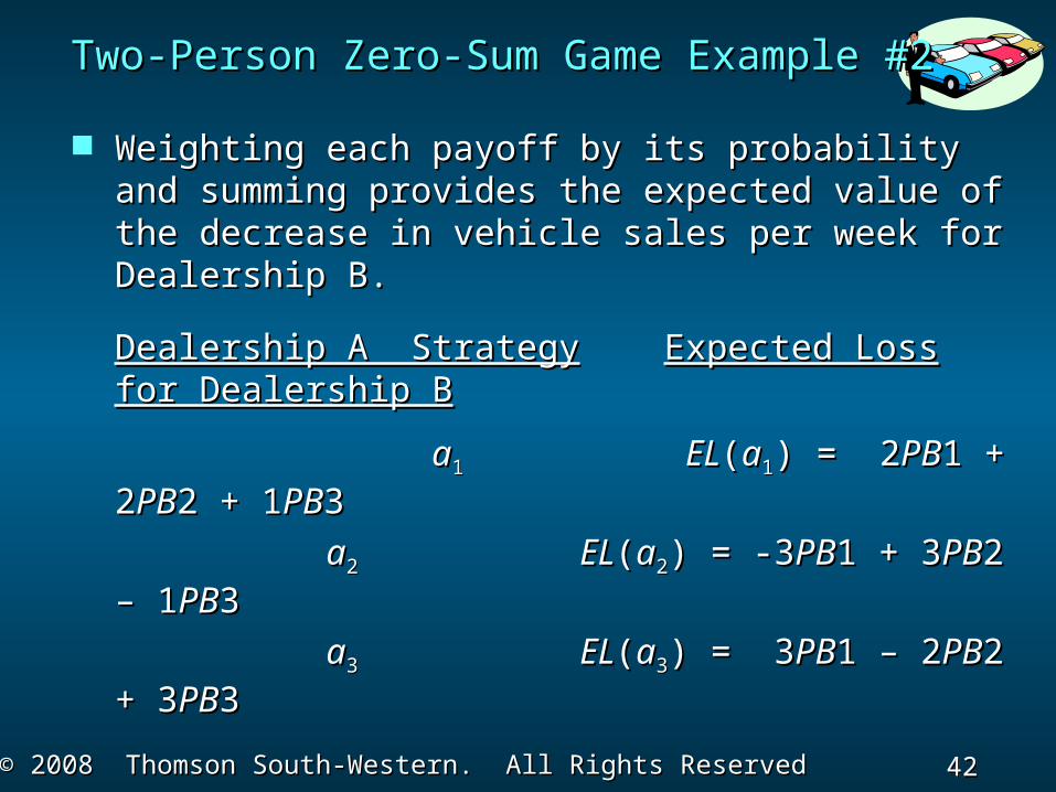
Weighting each payoff by its probability and Weighting each payoff by its probability and summing provides the expected value of the summing provides the expected value of the decrease in vehicle sales per week for Dealership decrease in vehicle sales per week for Dealership B.B.
Dealership A StrategyDealership A Strategy Expected Loss for Expected Loss for Dealership BDealership B
aa11 ELEL((aa11) = 2) = 2PBPB1 + 21 + 2PBPB2 + 2 + 11PBPB33
aa22 ELEL((aa22) = -3) = -3PBPB1 + 31 + 3PBPB2 – 2 – 11PBPB33
aa33 ELEL((aa33) = 3) = 3PBPB1 – 21 – 2PBPB2 + 2 + 33PBPB3 3
Two-Person Zero-Sum Game Example #2Two-Person Zero-Sum Game Example #2

43 43 Slide
Slide
© 2008 Thomson South-Western. All Rights Reserved© 2008 Thomson South-Western. All Rights Reserved
Two-Person Zero-Sum Game Example #2Two-Person Zero-Sum Game Example #2
Define Define LOSSBLOSSB to be the optimal expected loss in to be the optimal expected loss in vehicle sales for Dealership B, which we want to vehicle sales for Dealership B, which we want to minimize.minimize.
Thus, the individual expected losses, Thus, the individual expected losses, ELEL((aa11), ), ELEL((aa22) ) and and ELEL((aa33) must all be less than or equal to ) must all be less than or equal to LOSSBLOSSB..
For example,For example,
22PAPA1 + 21 + 2PAPA2 + 12 + 1PAPA3 3 << LOSSBLOSSB Also, the sum of Dealership B’s mixed strategy Also, the sum of Dealership B’s mixed strategy
probabilities must equal 1.probabilities must equal 1. This results in the LP formulation on the next slide This results in the LP formulation on the next slide
…..…..

44 44 Slide
Slide
© 2008 Thomson South-Western. All Rights Reserved© 2008 Thomson South-Western. All Rights Reserved
Dealership B’s Linear Programming FormulationDealership B’s Linear Programming Formulation
MinMin LOSSBLOSSB
s.t.s.t.
22PBPB1 + 21 + 2PBPB2 + 12 + 1PBPB3 – 3 – LOSSBLOSSB << 0 0 (Strategy (Strategy aa11))
-3-3PBPB1 + 31 + 3PBPB2 – 12 – 1PBPB3 – 3 – LOSSBLOSSB << 0 0 (Strategy (Strategy aa22))
33PBPB1 – 21 – 2PBPB2 + 32 + 3PBPB3 – 3 – LOSSBLOSSB << 0 0 (Strategy (Strategy aa33))
PBPB1 + 1 + PBPB2 + 2 + PBPB3 = 13 = 1 (Prob’s sum (Prob’s sum to 1)to 1)
PBPB1, 1, PBPB2, 2, PBPB3, 3, LOSSBLOSSB >> 0 0 (Non- (Non-negativity)negativity)
Two-Person Zero-Sum Game Example #2Two-Person Zero-Sum Game Example #2

45 45 Slide
Slide
© 2008 Thomson South-Western. All Rights Reserved© 2008 Thomson South-Western. All Rights Reserved
The Management ScientistThe Management Scientist Solution: Dealership Solution: Dealership BB
OBJECTIVE FUNCTION VALUE = 1.333OBJECTIVE FUNCTION VALUE = 1.333
VARIABLEVARIABLE VALUE VALUE REDUCED REDUCED COSTSCOSTS
PB1 PB1 0.000 0.000 0.833 0.833 PB2 PB2 0.333 0.333 0.000 0.000 PB3 PB3 0.667 0.667 0.000 0.000 LOSSBLOSSB 1.333 1.333 0.000 0.000
Two-Person Zero-Sum Game Example #2Two-Person Zero-Sum Game Example #2

46 46 Slide
Slide
© 2008 Thomson South-Western. All Rights Reserved© 2008 Thomson South-Western. All Rights Reserved
The Management ScientistThe Management Scientist Solution: Dealership Solution: Dealership BB
CONSTRAINTCONSTRAINT SLACK/SURPLUSSLACK/SURPLUS DUAL PRICESDUAL PRICES 1 1 0.000 0.000
0.8330.833 2 2 1.000 1.000
0.0000.000 3 3 0.000 0.000
0.1670.167 4 4 0.000 0.000 --
1.333 1.333
Two-Person Zero-Sum Game Example #2Two-Person Zero-Sum Game Example #2

47 47 Slide
Slide
© 2008 Thomson South-Western. All Rights Reserved© 2008 Thomson South-Western. All Rights Reserved
Dealership B’s Optimal Mixed StrategyDealership B’s Optimal Mixed Strategy
• Do not offer a cash rebate (Do not offer a cash rebate (bb11))• Offer free optional equipment (Offer free optional equipment (bb22) with a ) with a
probability of 0.333probability of 0.333• Offer a 0% loan (Offer a 0% loan (bb33) with a probability of 0.667) with a probability of 0.667
The expected payoff of this mixed strategy is a The expected payoff of this mixed strategy is a loss ofloss of1.333 vehicle sales per week for Dealership B.1.333 vehicle sales per week for Dealership B.
Note that expected loss for Dealership B is the Note that expected loss for Dealership B is the same assame asthe expected gain for Dealership A. (There is a the expected gain for Dealership A. (There is a
zero-zero-sum for the expected payoffs.)sum for the expected payoffs.)
Two-Person Zero-Sum Game Example #2Two-Person Zero-Sum Game Example #2

48 48 Slide
Slide
© 2008 Thomson South-Western. All Rights Reserved© 2008 Thomson South-Western. All Rights Reserved
Two-Person, Constant-Sum GamesTwo-Person, Constant-Sum Games
(The sum of the payoffs is a constant other (The sum of the payoffs is a constant other than zero.)than zero.)
Variable-Sum GamesVariable-Sum Games
(The sum of the payoffs is variable.)(The sum of the payoffs is variable.) nn-Person Games-Person Games
(A game involves more than two players.)(A game involves more than two players.) Cooperative GamesCooperative Games
(Players are allowed pre-play (Players are allowed pre-play communications.)communications.)
Infinite-Strategies GamesInfinite-Strategies Games
(An infinite number of strategies are available (An infinite number of strategies are available for the players.)for the players.)
Other Game Theory ModelsOther Game Theory Models

49 49 Slide
Slide
© 2008 Thomson South-Western. All Rights Reserved© 2008 Thomson South-Western. All Rights Reserved
End of Chapter 5End of Chapter 5