0&YHUVXV*DLQ6FKHGXOHG3,&RQWUROOHUIRU …

MODARES JOURNAL OF ELECTRICAL ENGINEERING, VOL 16, NO 4, WINTER 2016 1

1

Abstract— In recent years, wind energy becomes one of the

most important sources for electricity production. For instance

it is predicted that the installed wind capacity in China will be

about 40 GW till 2020. The permanent magnet synchronous

generators (PMSG) which contains of a permanent magnet that

causes DC excitation current in the windings, are widely used in

wind turbines. The advantage of this type of generators in

comparison to the others, are higher efficiency, controllable

terminal voltage and reactive power. It is also noticeable that the

PMSG speed can be controlled by the converter which leads to

MPPT implementation. The MPPT is always implemented to

control the generator speed and output power between the cut-

in and nominal wind speed. It is necessary to control the

generator speed by pitch or stall control for upper rated wind

speeds. In this paper after explaining the structure and

components of a typical wind turbine with permanent magnet

synchronous generator, designing of an offline DMC (Dynamic

Matrix Control) and a gain scheduled PI pitch controller are

presented. Both of these controllers have been tested on the

practical simulator of 100 KW wind turbine with PMSG

generator and the results are presented and compared.

Index Terms—Adaptive Control, DMC, PMSG, Pitch

Control.

I. INTRODUCTION

WIND turbine is a device that converts mechanical

energy captured from the wind into the electrical

power.Nowadays the wind turbines are manufactured in a

wide range of vertical and horizontal axis type. Arrays of

wind turbines, known as wind farms, are becoming an

important source of renewable energy and are used as part of

a strategy to reduce their reliance on fossil fuels [1].

Windmills were used in Iran as early as 200 B.C. and the

first practical windmills were built in Sistan. Nowadays a lot

of companies around the world are dealing with wind power

generation. Wind power, as an alternative to fossil fuels, is

plentiful, renewable, widely distributed, clean, produces

no greenhouse gas emissions during operation and uses little

land. The effects on the environment are generally less

problematic than those from other power sources. As of

2011, Denmark is generating more than a quarter of its

electricity from wind and 83 countries around the world are

using wind power to supply the electricity grid. In 2010 wind

energy production was over 2.5% of total worldwide

electricity usage, and growing rapidly at more than 25% per

annum [2].

Wind power is very consistent from year to year but has

Manuscript received December 15, 2016; accepted May 22, 2017

Nima Vaezi was with the School of Electrical Engineering, Ferdowsi

University of Mashhad. He is now with the Department of Avionic, University of Applied Science and Technology, Center of Mashhad Aviation

Training Center, Mashhad, Iran. (e-mail: [email protected]).

significant variation over shorter time scales. As the

proportion of wind power in a region increases, a need to

upgrade the grid, and a lowered ability to supplant

conventional production can occur. Power management

techniques such as having excess capacity storage,

geographically distributed turbines, dispatchable backing

sources, storage such as pumped-storage hydroelectricity,

exporting and importing power to neighboring areas or

reducing demand when wind production is low, can greatly

mitigate these problems. In addition, weather

forecasting permits the electricity network to be readied for

the predictable variations in production that occurs [3].

At the end of 2013, worldwide nominal capacity of wind-

powered generators was 318 GW, growing by 35 GW over

the preceding year. According to the World Wind Energy

Association, an industry organization, in 2010 wind power

generated 430 TWh or about 2.5% of worldwide electricity

usage, up from 1.5% in 2008 and 0.1% in 1997. Between

2005 and 2010 the average annual growth in new installations

was 27.6%. Wind power market penetration is expected to

reach 3.35% by 2013 and 8% by 2018 [2-3].

In this years, wind energy becomes one of the most

important sources for electricity production. In 2006 he

installed wind capacity in China was about 2600 MW and has

grown nearly 105% in comparison to the previous year. It is

also predicted that the installed wind capacity in China will

be about 40 GW till 2020[4].

In this paper after explaining the structure and components of

a typical wind turbine, the PI tuning method and DMC basis

are discussed and applied to pitch control design of a 100 KW

wind turbine. The designed controllers are utilized and

compared to regulation of the pitch angle in both simulation

and practical application.

II. WIND TURBINE COMPONENTS

As it is shown in figure 1, there are four main parts in a

wind turbine: the base, tower, nacelle and blades. Because of

the blade's special shape, the wind creates a package of

pressure as it passes behind the blade and causing the turbine

to rotate. The blades capture the mechanical power from the

wind and transmit it to an electrical generator located in the

nacelle. The tower contains the electrical conduits, supports

the nacelle, and provides access to the nacelle for

maintenance. The base which is made of concrete reinforced

with steel bars, supports the whole structure [1].

There are a generator and a gearbox in the nacelle. The blades

are attached to the generator through a series of gears. The

gears increase the rotational speed of the blades to the

P. Tavakoli was with the School of Electrical Engineering, Ferdowsi

University of Mashhad, 91755-1111 Mashhad, Iran. (e-mail:

[email protected]). S. K. Hosseini-Sani is with the School of Electrical Engineering,

Ferdowsi University of Mashhad, 91755-1111 Mashhad, Iran. (e-mail:

[email protected]).

DMC versus Gain Scheduled PI Controller for

Pitch Regulation of 100 KW Wind Turbine

Nima Vaezi, Parisa Tavakkoli, and Seyyed Kamal Hosseini-Sani

A

Dow

nloa

ded

from

mje

e.m

odar

es.a

c.ir

at 1

4:10

IRS

T o

n F

riday

Oct

ober

8th

202

1

https://mjee.modares.ac.ir/article-17-5787-en.html


generator speed range. A wind turbine gearbox must be

robust enough to handle the frequent changes in torque

caused by changes in the wind speed. Generators can be either

variable or fixed speed. Variable speed generators produce

electricity at a varying frequency, which must be corrected to

50 or 60Hz before it is fed onto the grid.

Fig.1. The wind turbine components.

The blades can be rotated around their axis to reduce the

amount of lift when wind speed increases over the rated. This

rotation is called pitch angle [2].

All wind turbines have a yaw drive system to face the

rotor into the wind and to unwind the cables that travel down

to the base of the tower. The yaw drive system consists of a

hydraulic or electric motor mounted on the nacelle. It

contains a brake in order to stop the turbine from turning and

stabilizing it during normal operation [5].

The wind turbine consists of a number of sensors to read

the speed and direction of the wind, levels of electrical power

generation, the rotor speed, the blades’ pitch angle and other

variables. A computer process the inputs to carry out the

normal operation of the wind turbine with a safety system

which can override the controller in an emergency. The safety

system protects the turbine from operating in dangerous

conditions and ensures that the power generated has the

proper frequency, voltage and current levels to be supplied to

the grid [6].

The wind turbines often produce AC current with erratic

voltage and frequency. Therefore an inverter is used to

convert the erratic AC to DC, then back to a smoother AC

which can be synchronized with the grid [5].

In the variable speed wind turbines with pitch controller

which are one of the most popular wind turbines, two types

of controller are used to fix and level the output power and

rotor speed in different operating regions. The block diagram

of this controllers is shown in figure 2. When the wind speed

is lower than the rated, the speed controller adjusts the rotor

speed so that the maximum power can be obtained from the

wind. In another word, the speed controller adjust the tip

speed ratio (𝜆) at its maximum point. When the wind speed is

upper than the rated, the pitch controller adjusts the rotor

speed at the rated value by increasing the pitch angle of the

blades. While the wind speed is lower than the rated value,

the pitch angle is controlled so that the maximum power can

be obtained from the wind energy [5]. The three main reasons

for pitch control system are:

Optimizing the output power of the system

Adjusting all system variables at their limits and stability

Minimizing the load effect on the mechanical

components

Wind turbine

and generator

Power

converter

Speed

controller

Pitch

controller

Wind

speed υw

Active and

reactive power

Power

set pointRotor speed

Cross coupling

β

Fig. 2. Two types of controller are used in variable speed wind turbines.

Pitch control limits the output power when the wind speed

is over the rated value. The PI controller is a widespread

method for adjusting the pitch angle. The actuators used in

the pitch system are often hydraulic servo motors. This

actuators provides a pitch transition rate about 5 to 10

degree/second.

The electrical power produced in the wind turbines are

related to the cube of the wind speed. The power coefficient

or 𝐶𝑝 shows the extractable part of the wind power and is a

function of tip speed ratio and pitch angle. In figure 3 the

mechanical power characteristics of a wind turbine is shown

as a function of rotor and wind speed [7].

The operating regions of the wind turbine system is shown in

figure 4. When the wind speed becomes more than the cut in

wind speed, the blades start to rotate. When wind speed

increases and becomes more than the rated value, the pitch

control system adjust the rotor speed at its rated value by

increasing the pitch angle. If the wind speed becomes more

than the cut out value, mechanical brakes forced the turbine

to stop [7]. While the wind energy is not constant and depends

on the wind speed, the output power of the wind turbines

changes with the cube of the wind speed. If the power

coefficient of wind turbine is very low, frequency changes

according to wind speed changes, are negligible. But if the

power coefficient of wind turbine is high, frequency changes

according to wind speed changes will increase [5].

Fig. 3. Mechanical power characteristics of a wind turbine [1].

Fig. 4. The operating regions of the wind turbine system [3].

Dow

nloa

ded

from

mje

e.m

odar

es.a

c.ir

at 1

4:10

IRS

T o

n F

riday

Oct

ober

8th

202

1


VAEZI et al. DMC VERSUS GAIN SCHEDULED PI CONTROLLER FOR PITCH REGULATION OF 100 KW WIND… 3

III. WIND TURBINE AND PERMANENT MAGNET

SYNCHRONOUS GENERATOR

The aerodynamic power produced by the turbine blades Pω,

can be calculated through by (1). In this equation ρ is the air

density, r is the rotor radius, v presents the wind speed and β

is the pitch angle. The power coefficient is calculated through

(2). In this equation ωm shows the angular rotor speed.

𝑃𝜔 =𝜌𝜋𝑟2𝜐3𝐶𝑝(𝜆, 𝜙)

2 (1)

𝜆 =𝑟𝜔𝑚

𝜐 (2)

The aerodynamic torque as shown in (3) is related to Pω

and ωm.

𝑇𝜔 =𝑃𝜔

𝜔𝑚

=𝜌𝜋𝑟3𝜐2𝐶𝑝(𝜆, 𝜙)

2𝜆 (3)

The drive model is shown in (4). In this equation ωe( ωe =Pωg = PNωm) is the electrical rotor speed and ωg is the

mechanical rotor speed. The number of the poles is shown

by P, turbine inertia is shown by J, N is shown the gearbox

Conversion ratio and Te is shown the electrical torque [8].

𝑒 =𝑃

𝐽(

𝑇𝜔

𝑁+ 𝑇𝑒) (4)

The permanent magnet synchronous generators (PMSG)

which contains of a permanent magnet that causes DC

excitation current in the windings, are widely used in wind

turbines. The advantage of this type of generators in

comparison to other types are higher efficiency, controllable

terminal voltage and reactive power. Besides these

advantages, having no resistance losses and no need for an

extra power supply to excite a generator are some of the

distinction of PMSG. Another advantage of PMSG is the

ability of bringing out the gearbox while increasing the

generator poles. This advantage decreases the mechanical

losses and costs [8].

Equation (5) shows the relation between voltage and torque

of a PMSG. In this equation ud and uq are voltage

components of direct and quadrature axis and id and iq are

current components of direct and quadrature axis, 𝑅𝑠 is the

stator resistance, 𝐿𝑑 and 𝐿𝑞 are inductance components of dq

axis and 𝜙 is the permanent magnetic flux.

𝑢𝑑 = 𝑅𝑠𝑖𝑑 +𝑑

𝑑𝑡𝐿𝑑𝑖𝑑 − 𝜔𝑒𝐿𝑞𝑖𝑞

𝑢𝑞 = 𝑅𝑠𝑖𝑞 +𝑑

𝑑𝑡𝐿𝑞𝑖𝑞 + 𝜔𝑒(𝐿𝑞𝑖𝑞 + 𝜙)

𝑇𝑒 =3

2𝑃 ((𝐿𝑑 − 𝐿𝑞)𝑖𝑑𝑖𝑞 + 𝜙𝑖𝑞)

(2)

If Ld = Lq = L then (5) can be written as (6).

𝑑𝑖𝑑

𝑑𝑡= −

𝑅𝑆

𝐿𝑖𝑑 + 𝜔𝑒𝑖𝑞 +

1

𝐿𝑢𝑑

𝑑𝑖𝑞

𝑑𝑡= −

𝑅𝑆

𝐿𝑖𝑞 − 𝜔𝑒𝑖𝑑 −

𝜔𝑒𝜙

𝐿+

1

𝐿𝑢𝑑

𝑇𝑒 =3

2𝑃𝜙𝑖𝑞

(6)

The 100KW wind turbine parameters are presented in table 1.

IV. MPPT AND CONVERTER CONTROL

Maximum power point tracking (MPPT) is a technique that

wind turbines solar battery chargers and similar devices use

TABLE 1.

THE 100KW WIND TURBINE PARAMETERS.

Name Symbol Value

Inertia J

70 (For practical

simulator)

1000 (For wind

turbine)

Friction Constant 𝐵 4.2

Gear Box Ratio 𝑁 5.91

Air Density 𝜌 1.05

Nominal Gird Power 𝑃𝐺𝑟𝑖𝑑 100 𝐾𝑊

Generator Inductance 𝐿 1 𝑚𝐻

Generator Resistance 𝑅𝑆 0.147 Ω

Permanent Magnetic flux 𝜙 2.1

Number of Pair Poles 𝑃 11

Rotor Radius 𝑅 13 𝑚

Pitch Rate --- 10 𝑑𝑔/𝑠𝑒𝑐

Proportional Gain of Convertor Speed

Controller 𝐾𝑝𝑝 1.24

Integral Gain of Convertor Speed

Controller 𝐾𝑝𝑖 4.95

Proportional Gain of Convertor Current

Controller 𝐾𝑝 3.675

Integral Gain of Convertor Current

Controller 𝐾𝑖 183.75

to obtain the maximum possible power from the power

source. In the wind turbine system, the MPPT procedure is

implemented by the convertor. MPPT procedure means

tracking a predefined curve which is obtained from Cp and

power coefficient characteristics of the wind turbine [9].

In the operational region 2 the MPPT curve should be

implemented and if the wind speed increases from rated, the

pitch mechanism acts to control the generator speed and

output power. The MPPT curve of the 100 KW wind turbine

produced in Sun and Air Research Institute is shown in

figure5.

There are some limitations on the designed 100 KW wind

turbine which are mentioned below.

Maximum available generator speed in the MPPT

curve is 325 rpm.

Maximum sustainable generator speed for the

convertor is 350 rpm and the generator speed more

than 350 rpm is sustainable for about 3 or 4 seconds.

In the operating point the generator torque is 2800

N.m.

Maximum grid power selected on the MPPT curve

is equal to 84 KW. When the generator speed

reached to the 325 rpm, the grid power will be within

the sustainable power for the convertor which is

about 101 KW.

Because of this limitations pitch control of this wind turbine

is not feasible with a simple PI controller. Therefore it is

necessary to apply a new method.

Fig. 5. The MPPT curve of the 100 KW wind turbine produced in Sun and Air Research Institute.

100 150 200 250 300 3500

2

4

6

8

10x 10

4

Generator Speed (rpm)

Mec

hani

cal P

ower

(Wat

t)

Dow

nloa

ded

from

mje

e.m

odar

es.a

c.ir

at 1

4:10

IRS

T o

n F

riday

Oct

ober

8th

202

1



In figure 6 the pitch control system based on the generator

speed error is shown. The generator speed measured by

sensors is compared with the rated generator speed and the

difference is applied to the PI controller. The controller

output is the reference value of the pitch angle. The pitch

angle reference value is compared with the measured pitch

angle and the pitch command is applied to the pitch actuator.

Hydraulic actuators or servo motors can be used as the pitch

actuator in wind turbines.

The proportional and integral gains of the PI controller is

extracted by using the first order Ziegler Nichols method. For

the first step the generator speed is fixed on 350 rpm in wind

9.175 m/s by applying pitch angle about 0.5 degree of the

pitch angle. The pitch angle changed from 0.5 to 1 degree

suddenly and according to the step response of the generator

speed, the proportional and integral gain of the PI controller

will be designed. The generator speed step response is plotted

in figure 7 for the Simulink file.

+ +

-

-Generator Speed

ωmeans

Rated Speed

ωref

errorPI

Pitch

servo

Wind

turbine

βref

Fig. 6. Pitch angle control based on the generator speed error.

Fig. 7. The generator speed step response.

According to the first order Ziegler Nichols method, at this

wind speed, the gain 𝐾 and the time constant 𝜏 and the delay

𝜏𝑑 in (7) are calculated as 𝐾 = 0.3527 , 𝜏 = 0.69041 and

𝜏𝑑 = 0.2.

𝐺𝑓𝑖𝑟𝑠𝑡 𝑜𝑟𝑑𝑒𝑟 =𝐾

𝜏𝑠 + 1𝑒−𝜏𝑑𝑠 (7)

Therefore the controller gain is equal to 𝐾𝑃 = 8.808 and the

integrator time constant is equal to 𝑇𝑖 = 0.66. The transfer

function of the controller is as shown in (8).

𝐺𝑐𝑜𝑛𝑡𝑟𝑜𝑙 = 𝐾𝑃 (1 +1

𝜏𝑖𝑠) (8)

This test is repeated at different wind speeds and the

controller gains and the integrator time constants are

calculated for different wind regions. The table 2 which is

extracted from this collection of tests, contains 𝐾, 𝜏, 𝜏𝑑,

𝐾𝑃 , 𝑇𝑖 , pitch angle to control the generator speed at 350 rpm

and pitch angle to control the generator speed at 325 rpm for

different wind speeds.

The wind region is recognized based on the current pitch

signal. In different wind region the pitch controller increases

the pitch angle to stabilize the generator speed at 325 rpm.

Therefore the current pitch angle specifies the wind region.

Because of simplicity 𝑇𝑖 is supposed to be fixed in 0.5 second

and the controller gain will be determined according to the

current pitch angle based on the data represented by table 2.

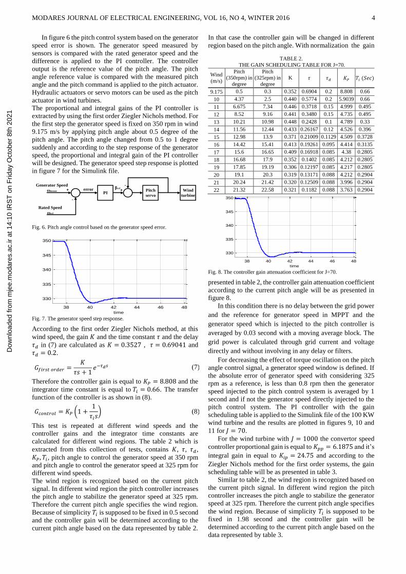
In that case the controller gain will be changed in different

region based on the pitch angle. With normalization the gain

TABLE 2.

THE GAIN SCHEDULING TABLE FOR J=70.

Wind

(m/s)

Pitch (350rpm) in

degree

Pitch (325rpm) in

degree

K 𝜏 𝜏𝑑 𝐾𝑃 𝑇𝑖 (𝑆𝑒𝑐)

9.175 0.5 0.3 0.352 0.6904 0.2 8.808 0.66

10 4.37 2.5 0.440 0.5774 0.2 5.9039 0.66

11 6.675 7.34 0.446 0.3718 0.15 4.999 0.495

12 8.52 9.16 0.441 0.3480 0.15 4.735 0.495

13 10.21 10.98 0.448 0.2428 0.1 4.789 0.33

14 11.56 12.44 0.433 0.26167 0.12 4.526 0.396

15 12.98 13.9 0.371 0.21009 0.1129 4.509 0.3728

16 14.42 15.41 0.413 0.19261 0.095 4.414 0.3135

17 15.6 16.65 0.409 0.16918 0.085 4.38 0.2805

18 16.68 17.9 0.352 0.1402 0.085 4.212 0.2805

19 17.85 19.19 0.306 0.12197 0.085 4.217 0.2805

20 19.1 20.3 0.319 0.13171 0.088 4.212 0.2904

21 20.24 21.42 0.320 0.12509 0.088 3.996 0.2904

22 21.32 22.58 0.321 0.1182 0.088 3.763 0.2904

Fig. 8. The controller gain attenuation coefficient for J=70.

presented in table 2, the controller gain attenuation coefficient

according to the current pitch angle will be as presented in

figure 8.

In this condition there is no delay between the grid power

and the reference for generator speed in MPPT and the

generator speed which is injected to the pitch controller is

averaged by 0.03 second with a moving average block. The

grid power is calculated through grid current and voltage

directly and without involving in any delay or filters.

For decreasing the effect of torque oscillation on the pitch

angle control signal, a generator speed window is defined. If

the absolute error of generator speed with considering 325

rpm as a reference, is less than 0.8 rpm then the generator

speed injected to the pitch control system is averaged by 1

second and if not the generator speed directly injected to the

pitch control system. The PI controller with the gain

scheduling table is applied to the Simulink file of the 100 KW

wind turbine and the results are plotted in figures 9, 10 and

11 for 𝐽 = 70.

For the wind turbine with 𝐽 = 1000 the convertor speed

controller proportional gain is equal to 𝐾𝑝𝑝 = 6.1875 and it’s

integral gain in equal to 𝐾𝑖𝑝 = 24.75 and according to the

Ziegler Nichols method for the first order systems, the gain

scheduling table will be as presented in table 3.

Similar to table 2, the wind region is recognized based on

the current pitch signal. In different wind region the pitch

controller increases the pitch angle to stabilize the generator

speed at 325 rpm. Therefore the current pitch angle specifies

the wind region. Because of simplicity 𝑇𝑖 is supposed to be

fixed in 1.98 second and the controller gain will be

determined according to the current pitch angle based on the

data represented by table 3.

38 40 42 44 46 48

330

335

340

345

350

time

38 40 42 44 46 48

330

335

340

345

350

time

Dow

nloa

ded

from

mje

e.m

odar

es.a

c.ir

at 1

4:10

IRS

T o

n F

riday

Oct

ober

8th

202

1



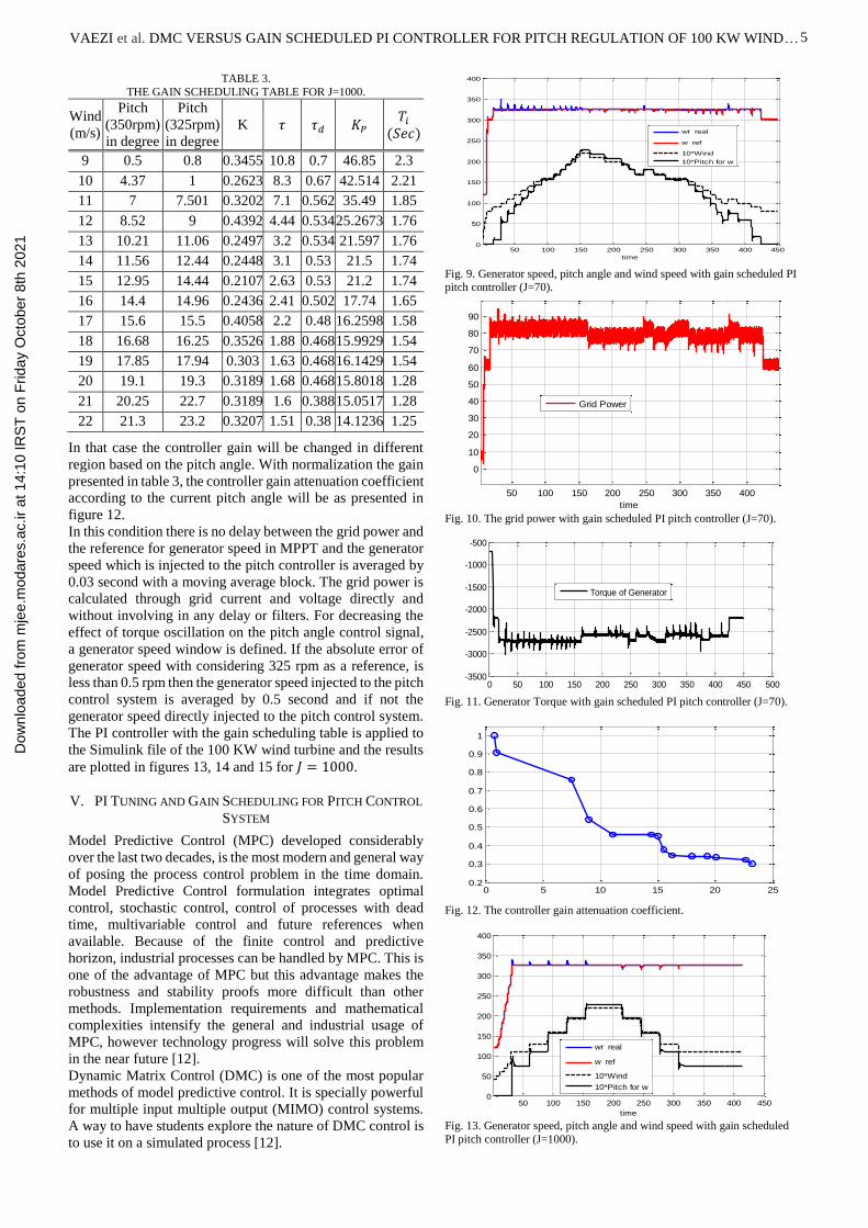
TABLE 3.

THE GAIN SCHEDULING TABLE FOR J=1000.

Wind

(m/s)

Pitch

(350rpm)

in degree

Pitch

(325rpm)

in degree

K 𝜏 𝜏𝑑 𝐾𝑃 𝑇𝑖

(𝑆𝑒𝑐)

9 0.5 0.8 0.3455 10.8 0.7 46.85 2.3

10 4.37 1 0.2623 8.3 0.67 42.514 2.21

11 7 7.501 0.3202 7.1 0.562 35.49 1.85

12 8.52 9 0.4392 4.44 0.534 25.2673 1.76

13 10.21 11.06 0.2497 3.2 0.534 21.597 1.76

14 11.56 12.44 0.2448 3.1 0.53 21.5 1.74

15 12.95 14.44 0.2107 2.63 0.53 21.2 1.74

16 14.4 14.96 0.2436 2.41 0.502 17.74 1.65

17 15.6 15.5 0.4058 2.2 0.48 16.2598 1.58

18 16.68 16.25 0.3526 1.88 0.468 15.9929 1.54

19 17.85 17.94 0.303 1.63 0.468 16.1429 1.54

20 19.1 19.3 0.3189 1.68 0.468 15.8018 1.28

21 20.25 22.7 0.3189 1.6 0.388 15.0517 1.28

22 21.3 23.2 0.3207 1.51 0.38 14.1236 1.25

In that case the controller gain will be changed in different

region based on the pitch angle. With normalization the gain

presented in table 3, the controller gain attenuation coefficient

according to the current pitch angle will be as presented in

figure 12.

In this condition there is no delay between the grid power and

the reference for generator speed in MPPT and the generator

speed which is injected to the pitch controller is averaged by

0.03 second with a moving average block. The grid power is

calculated through grid current and voltage directly and

without involving in any delay or filters. For decreasing the

effect of torque oscillation on the pitch angle control signal,

a generator speed window is defined. If the absolute error of

generator speed with considering 325 rpm as a reference, is

less than 0.5 rpm then the generator speed injected to the pitch

control system is averaged by 0.5 second and if not the

generator speed directly injected to the pitch control system.

The PI controller with the gain scheduling table is applied to

the Simulink file of the 100 KW wind turbine and the results

are plotted in figures 13, 14 and 15 for 𝐽 = 1000.

V. PI TUNING AND GAIN SCHEDULING FOR PITCH CONTROL

SYSTEM

Model Predictive Control (MPC) developed considerably

over the last two decades, is the most modern and general way

of posing the process control problem in the time domain.

Model Predictive Control formulation integrates optimal

control, stochastic control, control of processes with dead

time, multivariable control and future references when

available. Because of the finite control and predictive

horizon, industrial processes can be handled by MPC. This is

one of the advantage of MPC but this advantage makes the

robustness and stability proofs more difficult than other

methods. Implementation requirements and mathematical

complexities intensify the general and industrial usage of

MPC, however technology progress will solve this problem

in the near future [12].

Dynamic Matrix Control (DMC) is one of the most popular

methods of model predictive control. It is specially powerful

for multiple input multiple output (MIMO) control systems.

A way to have students explore the nature of DMC control is

to use it on a simulated process [12].

Fig. 9. Generator speed, pitch angle and wind speed with gain scheduled PI pitch controller (J=70).

Fig. 10. The grid power with gain scheduled PI pitch controller (J=70).

Fig. 11. Generator Torque with gain scheduled PI pitch controller (J=70).

Fig. 12. The controller gain attenuation coefficient.

Fig. 13. Generator speed, pitch angle and wind speed with gain scheduled

PI pitch controller (J=1000).

50 100 150 200 250 300 350 400 4500

50

100

150

200

250

300

350

400

time

wr real

w ref

10*Wind

10*Pitch for w

50 100 150 200 250 300 350 400

0

10

20

30

40

50

60

70

80

90

time

Grid Power

0 50 100 150 200 250 300 350 400 450 500-3500

-3000

-2500

-2000

-1500

-1000

-500

Torque of Generator

0 5 10 15 20 250.2

0.3

0.4

0.5

0.6

0.7

0.8

0.9

1

50 100 150 200 250 300 350 400 4500

50

100

150

200

250

300

350

400

time

wr real

w ref

10*Wind

10*Pitch for w

Dow

nloa

ded

from

mje

e.m

odar

es.a

c.ir

at 1

4:10

IRS

T o

n F

riday

Oct

ober

8th

202

1



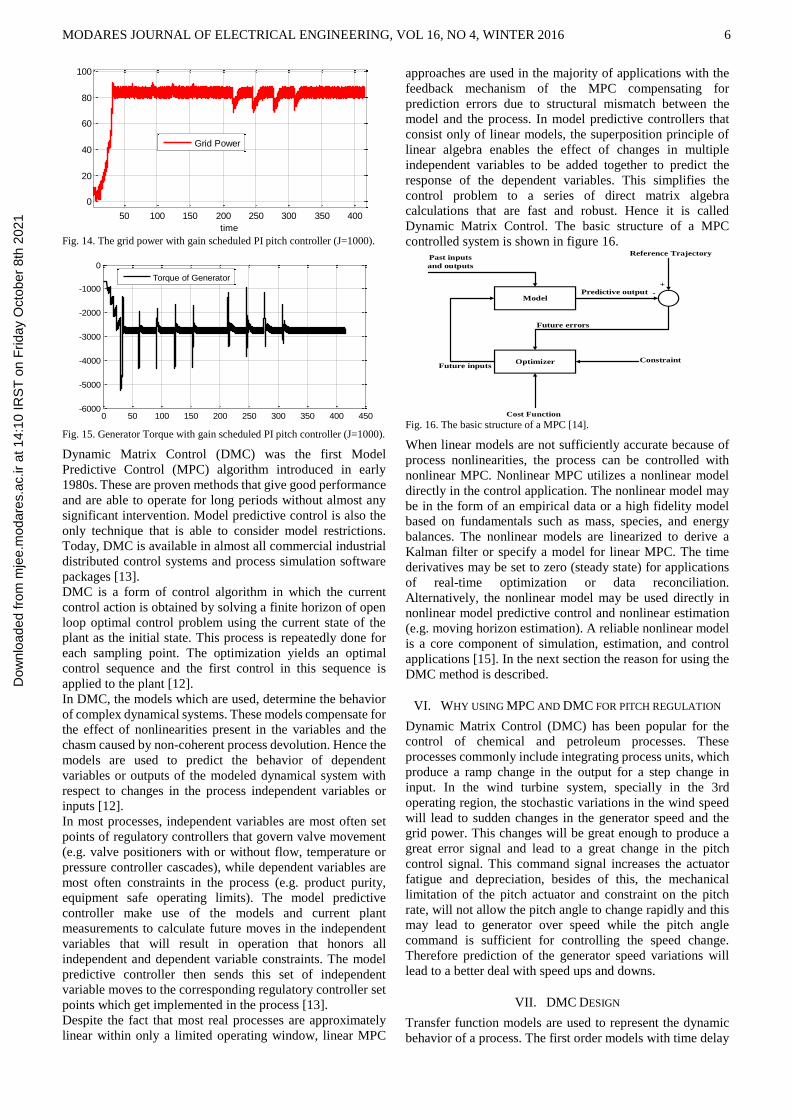
Fig. 14. The grid power with gain scheduled PI pitch controller (J=1000).

Fig. 15. Generator Torque with gain scheduled PI pitch controller (J=1000).

Dynamic Matrix Control (DMC) was the first Model

Predictive Control (MPC) algorithm introduced in early

1980s. These are proven methods that give good performance

and are able to operate for long periods without almost any

significant intervention. Model predictive control is also the

only technique that is able to consider model restrictions.

Today, DMC is available in almost all commercial industrial

distributed control systems and process simulation software

packages [13].

DMC is a form of control algorithm in which the current

control action is obtained by solving a finite horizon of open

loop optimal control problem using the current state of the

plant as the initial state. This process is repeatedly done for

each sampling point. The optimization yields an optimal

control sequence and the first control in this sequence is

applied to the plant [12].

In DMC, the models which are used, determine the behavior

of complex dynamical systems. These models compensate for

the effect of nonlinearities present in the variables and the

chasm caused by non-coherent process devolution. Hence the

models are used to predict the behavior of dependent

variables or outputs of the modeled dynamical system with

respect to changes in the process independent variables or

inputs [12].

In most processes, independent variables are most often set

points of regulatory controllers that govern valve movement

(e.g. valve positioners with or without flow, temperature or

pressure controller cascades), while dependent variables are

most often constraints in the process (e.g. product purity,

equipment safe operating limits). The model predictive

controller make use of the models and current plant

measurements to calculate future moves in the independent

variables that will result in operation that honors all

independent and dependent variable constraints. The model

predictive controller then sends this set of independent

variable moves to the corresponding regulatory controller set

points which get implemented in the process [13].

Despite the fact that most real processes are approximately

linear within only a limited operating window, linear MPC

approaches are used in the majority of applications with the

feedback mechanism of the MPC compensating for

prediction errors due to structural mismatch between the

model and the process. In model predictive controllers that

consist only of linear models, the superposition principle of

linear algebra enables the effect of changes in multiple

independent variables to be added together to predict the

response of the dependent variables. This simplifies the

control problem to a series of direct matrix algebra

calculations that are fast and robust. Hence it is called

Dynamic Matrix Control. The basic structure of a MPC

controlled system is shown in figure 16.

Model

Optimizer

Cost Function

ConstraintFuture inputs

Future errors

Predictive output

Past inputs

and outputs

Reference Trajectory

+

-

Fig. 16. The basic structure of a MPC [14].

When linear models are not sufficiently accurate because of

process nonlinearities, the process can be controlled with

nonlinear MPC. Nonlinear MPC utilizes a nonlinear model

directly in the control application. The nonlinear model may

be in the form of an empirical data or a high fidelity model

based on fundamentals such as mass, species, and energy

balances. The nonlinear models are linearized to derive a

Kalman filter or specify a model for linear MPC. The time

derivatives may be set to zero (steady state) for applications

of real-time optimization or data reconciliation.

Alternatively, the nonlinear model may be used directly in

nonlinear model predictive control and nonlinear estimation

(e.g. moving horizon estimation). A reliable nonlinear model

is a core component of simulation, estimation, and control

applications [15]. In the next section the reason for using the

DMC method is described.

VI. WHY USING MPC AND DMC FOR PITCH REGULATION

Dynamic Matrix Control (DMC) has been popular for the

control of chemical and petroleum processes. These

processes commonly include integrating process units, which

produce a ramp change in the output for a step change in

input. In the wind turbine system, specially in the 3rd

operating region, the stochastic variations in the wind speed

will lead to sudden changes in the generator speed and the

grid power. This changes will be great enough to produce a

great error signal and lead to a great change in the pitch

control signal. This command signal increases the actuator

fatigue and depreciation, besides of this, the mechanical

limitation of the pitch actuator and constraint on the pitch

rate, will not allow the pitch angle to change rapidly and this

may lead to generator over speed while the pitch angle

command is sufficient for controlling the speed change.

Therefore prediction of the generator speed variations will

lead to a better deal with speed ups and downs.

VII. DMC DESIGN

Transfer function models are used to represent the dynamic

behavior of a process. The first order models with time delay

50 100 150 200 250 300 350 400

0

20

40

60

80

100

time

Grid Power

0 50 100 150 200 250 300 350 400 450-6000

-5000

-4000

-3000

-2000

-1000

0

Torque of Generator

Dow

nloa

ded

from

mje

e.m

odar

es.a

c.ir

at 1

4:10

IRS

T o

n F

riday

Oct

ober

8th

202

1



are normally used for modeling different kinds of process.

Transfer function models need the order to be specified. Here

another way is to use a “discrete response model”. It has the

advantage that the model coefficients can be obtained directly

from the state response which can be represented as (9).

𝑥(𝑘 + 1) − 𝐴𝑥(𝑘) + 𝑏𝑢(𝑘),𝑦(𝑘 + 1) = 𝐶𝑥(𝑘)

(9)

Here 𝑥(𝑘) is the input at instant 𝑘, 𝑢(𝑘) is the unit step

function and 𝑥(𝑘 + 1) and 𝑦(𝑘 + 1) are the input and output

at the next step. In equation (9) 𝐴, 𝐵 and 𝐶 are the state space

coefficient of the model [12].

With considering the control horizon 𝑁𝑢 as the number of the

control actions that are taken in a model with predictive

horizon of 𝑁𝑝, the vector presented in (10), represents the

state response coefficient vector.

= [𝑎1 𝑎2 𝑎3 … 𝑎𝑁]𝑇 (10)

If the current time instant is 𝑘 the control action has to be

taken at time instant 𝑘 − 1. The predicted output of the

process at instant 𝑘 can be represented by (11).

𝑦(𝑘) = ∑ 𝑎𝑖Δ𝑢(𝑘 − 1) + 𝑎𝑠𝑠𝑢(𝑘 − 𝑁 − 1)

𝑁

𝑖−1

+ 𝑑(𝑘)

(11)

In equation (11), 𝑑(𝑘) is the effect of disturbance and 𝑎𝑠𝑠 is

the state response coefficient for the steady state situation.

The above equation can be written as (12).

𝑑(𝑘) = 𝑦𝑚𝑒𝑎𝑠𝑢𝑟𝑒𝑑 − ∑ 𝑎𝑖Δ𝑢(𝑘 − 1)

𝑁

𝑖−1

+ 𝑎𝑠𝑠𝑢(𝑘 − 𝑁 − 1)

(12)

For one step ahead prediction, equation (12) can be written as

𝑦(𝑘 + 1) = 𝑎1Δ𝑢(𝑘) + 𝑎2Δ𝑢(𝑘 − 1) + ⋯+ 𝑎𝑠𝑠Δ𝑢(𝑘 − 𝑁 − 1) + 𝑑(𝑘)

(13)

With this assuming that disturbance 𝑑(𝑘) is constant for all

values of prediction variables. Since prediction horizon is

greater than one, with generalization the above equation can

be written as (14).

𝑢(𝑘 + 𝑁) = 𝑦𝑝𝑎𝑠𝑡 + 𝐴Δ𝑢(𝑘) + 𝐷 (14)

To get the perfect output, it can be supposed that 𝑦𝑠𝑝 = 𝑦(𝑘 +

1). Hence the variation of control signal can be represented

as (15).

Δ𝑢 = 𝐴−1(𝑦𝑠𝑝 − 𝑦𝑝𝑎𝑠𝑡 − 𝐷) (15)

The equation (15) is the control law for DMC method. Every

controller design has some design parameters, which can be

tuned to get the desired response of the controller. These

parameters are called the tuning parameters of the controller.

The following guidelines are basically used to tune a DMC:

1- The model horizon 𝑁 should be selected so that 𝑁Δ𝑡 will

be greater than open loop settling time. Values of N is

normally taken between 20 to70. In our design it is

selected to 20.

2- The prediction horizon 𝑁𝑝 determines how far into the

future the control objective is reached. Increasing 𝑁𝑝

makes the control more accurate but increases the

computation. The most recommended value of 𝑁𝑝 is

when 𝑁𝑝 = 𝑁 + 𝑁𝑢.

3- The control horizon 𝑁𝑢 determine the number of the

control actions calculated into the future. Too large value

of 𝑁𝑢 causes excessive control action. Small value of

𝑁𝑢 makes the controller insensitive of noise [12].

VIII. DESIGN, SIMULATION AND TEST OF THE DMC

METHOD

To design the dynamic matrix controller for the pitch

control system, the model horizon is selected to 20 and the

first order transfer function obtained from the test described

in figure 7 for the Ziegler Nichols method, is used. The

transfer function is converted to a state space model and the

DMC control law is calculated for different initial conditions.

These initial conditions are initial speed and the error signal

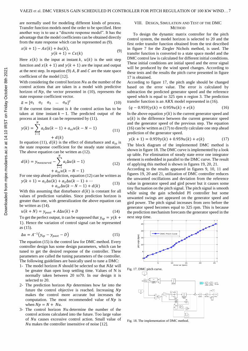
will be produced by the wind speed changes. According to

these tests and the results the pitch curve presented in figure

17 is obtained.

According to figure 17, the pitch angle should be changed

based on the error value. The error is calculated by

subtraction the predicted generator speed and the reference

speed which is equal to 325 rpm n region 3. The prediction

transfer function is an ARX model represented in (16).

(𝑞 − 0.959)𝑦(𝑘) = 0.959𝑢(𝑘) + 𝑒(𝑘) (16)

In the above equation 𝑦(𝑘) is the current generator speed and

𝑢(𝑘) is the difference between the current generator speed

and the generator speed of the previous step. The equation

(16) can be written as (17) to directly calculate one step ahead

prediction of the generator speed.

𝑦(𝑘 + 1) = 0.959𝑦(𝑘) + 0.959𝑢(𝑘) + 𝑒(𝑘) (17)

The block diagram of the implemented DMC method is

shown in figure 18. The DMC curve is implemented by a look

up table. For elimination of steady state error one integrator

element is embedded in parallel to the DMC curve. The result

of applying this method is shown in figures 19, 20, 21.

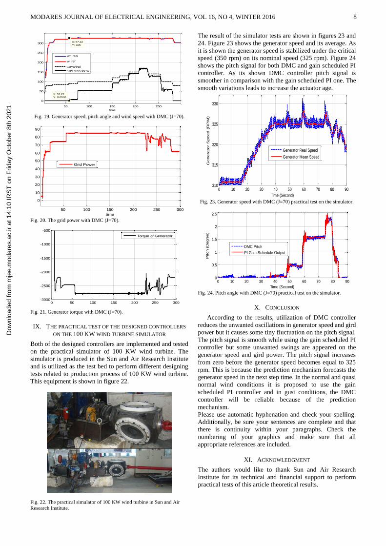
According to the results appeared in figures 9, 10, 11 and

figures 19, 20 and 21, utilization of DMC controller reduces

the unwanted oscillations and deviation from the reference

value in generator speed and gird power but it causes some

tiny fluctuation on the pitch signal. The pitch signal is smooth

while using the gain scheduled PI controller but some

unwanted swings are appeared on the generator speed and

gird power. The pitch signal increases from zero before the

generator speed becomes equal to 325 rpm. This is because

the prediction mechanism forecasts the generator speed in the

next step time.

Fig. 17. DMC pitch curve.

Fig. 18. The implementation of DMC method.

5 10 15 20 25

0

5

10

15

20

25

Error wr (rpm)

pitc

h an

gle

(dgr

ee)

DMC Pitch Curve

Dow

nloa

ded

from

mje

e.m

odar

es.a

c.ir

at 1

4:10

IRS

T o

n F

riday

Oct

ober

8th

202

1



Fig. 19. Generator speed, pitch angle and wind speed with DMC (J=70).

Fig. 20. The grid power with DMC (J=70).

Fig. 21. Generator torque with DMC (J=70).

IX. THE PRACTICAL TEST OF THE DESIGNED CONTROLLERS

ON THE 100 KW WIND TURBINE SIMULATOR

Both of the designed controllers are implemented and tested

on the practical simulator of 100 KW wind turbine. The

simulator is produced in the Sun and Air Research Institute

and is utilized as the test bed to perform different designing

tests related to production process of 100 KW wind turbine.

This equipment is shown in figure 22.

Fig. 22. The practical simulator of 100 KW wind turbine in Sun and Air

Research Institute.

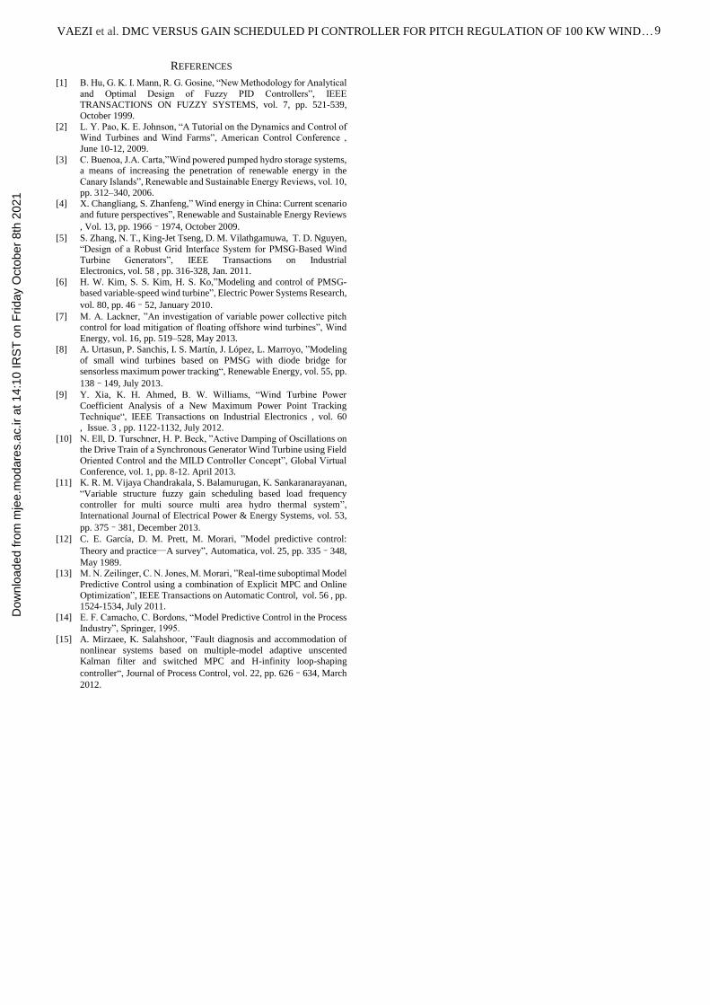
The result of the simulator tests are shown in figures 23 and

24. Figure 23 shows the generator speed and its average. As

it is shown the generator speed is stabilized under the critical

speed (350 rpm) on its nominal speed (325 rpm). Figure 24

shows the pitch signal for both DMC and gain scheduled PI

controller. As its shown DMC controller pitch signal is

smoother in comparison with the gain scheduled PI one. The

smooth variations leads to increase the actuator age.

Fig. 23. Generator speed with DMC (J=70) practical test on the simulator.

Fig. 24. Pitch angle with DMC (J=70) practical test on the simulator.

X. CONCLUSION

According to the results, utilization of DMC controller

reduces the unwanted oscillations in generator speed and gird

power but it causes some tiny fluctuation on the pitch signal.

The pitch signal is smooth while using the gain scheduled PI

controller but some unwanted swings are appeared on the

generator speed and gird power. The pitch signal increases

from zero before the generator speed becomes equal to 325

rpm. This is because the prediction mechanism forecasts the

generator speed in the next step time. In the normal and quasi

normal wind conditions it is proposed to use the gain

scheduled PI controller and in gust conditions, the DMC

controller will be reliable because of the prediction

mechanism.

Please use automatic hyphenation and check your spelling.

Additionally, be sure your sentences are complete and that

there is continuity within your paragraphs. Check the

numbering of your graphics and make sure that all

appropriate references are included.

XI. ACKNOWLEDGMENT

The authors would like to thank Sun and Air Research

Institute for its technical and financial support to perform

practical tests of this article theoretical results.

50 100 150 200 250

0

50

100

150

200

250

300

X: 57.22

Y: 0.0536

time

X: 57.22

Y: 325

wr real

w ref

10*Wind

10*Pitch for w

50 100 150 200 250 300

0

10

20

30

40

50

60

70

80

90

time

Grid Power

0 50 100 150 200 250 300-3000

-2500

-2000

-1500

-1000

-500

Torque of Generator

0 10 20 30 40 50 60 70 80 90310

315

320

325

330

Time (Second)

Genera

tor

Speed (

RP

M)

Generator Real Speed

Generator Mean Speed

0 10 20 30 40 50 60 70 80 900

0.5

1

1.5

2

2.5

Time (Second)

Pitch (

Degre

e)

DMC Pitch

PI Gain Schedule Output

Dow

nloa

ded

from

mje

e.m

odar

es.a

c.ir

at 1

4:10

IRS

T o

n F

riday

Oct

ober

8th

202

1



REFERENCES

[1] B. Hu, G. K. I. Mann, R. G. Gosine, “New Methodology for Analytical

and Optimal Design of Fuzzy PID Controllers”, IEEE TRANSACTIONS ON FUZZY SYSTEMS, vol. 7, pp. 521-539,

October 1999.

[2] L. Y. Pao, K. E. Johnson, “A Tutorial on the Dynamics and Control of Wind Turbines and Wind Farms”, American Control Conference ,

June 10-12, 2009.

[3] C. Buenoa, J.A. Carta,”Wind powered pumped hydro storage systems, a means of increasing the penetration of renewable energy in the

Canary Islands”, Renewable and Sustainable Energy Reviews, vol. 10,

pp. 312–340, 2006. [4] X. Changliang, S. Zhanfeng,” Wind energy in China: Current scenario

and future perspectives”, Renewable and Sustainable Energy Reviews

, Vol. 13, pp. 1966–1974, October 2009.

[5] S. Zhang, N. T., King-Jet Tseng, D. M. Vilathgamuwa, T. D. Nguyen,

“Design of a Robust Grid Interface System for PMSG-Based Wind

Turbine Generators”, IEEE Transactions on Industrial Electronics, vol. 58 , pp. 316-328, Jan. 2011.

[6] H. W. Kim, S. S. Kim, H. S. Ko,”Modeling and control of PMSG-

based variable-speed wind turbine”, Electric Power Systems Research,

vol. 80, pp. 46–52, January 2010.

[7] M. A. Lackner, ”An investigation of variable power collective pitch control for load mitigation of floating offshore wind turbines”, Wind

Energy, vol. 16, pp. 519–528, May 2013.

[8] A. Urtasun, P. Sanchis, I. S. Martín, J. López, L. Marroyo, ”Modeling of small wind turbines based on PMSG with diode bridge for

sensorless maximum power tracking“, Renewable Energy, vol. 55, pp.

138–149, July 2013.

[9] Y. Xia, K. H. Ahmed, B. W. Williams, “Wind Turbine Power

Coefficient Analysis of a New Maximum Power Point Tracking Technique“, IEEE Transactions on Industrial Electronics , vol. 60

, Issue. 3 , pp. 1122-1132, July 2012.

[10] N. Ell, D. Turschner, H. P. Beck, ”Active Damping of Oscillations on the Drive Train of a Synchronous Generator Wind Turbine using Field

Oriented Control and the MILD Controller Concept”, Global Virtual

Conference, vol. 1, pp. 8-12. April 2013. [11] K. R. M. Vijaya Chandrakala, S. Balamurugan, K. Sankaranarayanan,

“Variable structure fuzzy gain scheduling based load frequency

controller for multi source multi area hydro thermal system”, International Journal of Electrical Power & Energy Systems, vol. 53,

pp. 375–381, December 2013.

[12] C. E. García, D. M. Prett, M. Morari, ”Model predictive control:

Theory and practice—A survey”, Automatica, vol. 25, pp. 335–348,

May 1989. [13] M. N. Zeilinger, C. N. Jones, M. Morari, ”Real-time suboptimal Model

Predictive Control using a combination of Explicit MPC and Online

Optimization”, IEEE Transactions on Automatic Control, vol. 56 , pp. 1524-1534, July 2011.

[14] E. F. Camacho, C. Bordons, “Model Predictive Control in the Process Industry”, Springer, 1995.

[15] A. Mirzaee, K. Salahshoor, ”Fault diagnosis and accommodation of

nonlinear systems based on multiple-model adaptive unscented Kalman filter and switched MPC and H-infinity loop-shaping

controller“, Journal of Process Control, vol. 22, pp. 626–634, March

2012.

Dow

nloa

ded

from

mje

e.m

odar

es.a

c.ir

at 1

4:10

IRS

T o

n F

riday

Oct

ober

8th

202

1


Documents

0&YHUVXV*DLQ6FKHGXOHG3,&RQWUROOHUIRU …