09_EPES_Probabilistic Load Flow With Wind Production Uncertainty

8/8/2019 09_EPES_Probabilistic Load Flow With Wind Production Uncertainty

http://slidepdf.com/reader/full/09epesprobabilistic-load-flow-with-wind-production-uncertainty 1/8



method has better convergence properties, without more compu-tational burden.

The method is applied to next day operation of systems withgreat wind penetration. Usually, the system operators of these net-works use the output of a short term wind power prediction pro-gram to forecast the next day grid constraints and congestions.However, these predictions have a lower accuracy than load fore-

casts, and their uncertainty should be also taken into account, forinstance for the available interconnection capacity between sys-tems. Therefore, a tool able to assess the probability of surpassingthe allowed line capacity is very practical for an adequateoperation.

The paper is structured as follows: first, a short view of shortterm wind power prediction, and the uncertainty associated toits output, is given. Then, the theoretical foundations of the Cor-nish–Fisher expansion series and the necessary definitions areintroduced. The method is applied to a test grid, and its resultsare compared to those obtained using Gram–Charlier expansionseries. A summary with the main conclusions ends the paper.

2. Short term wind power prediction: uncertainty

2.1. Short term wind power prediction

Short term wind power prediction programs are tools that pro-vide an estimate of the future power production of a wind farm, ora group of wind farms, in the next hours. For this purpose, they usemeteorological forecasts coming from a Numerical Weather Pre-diction (NWP) tool, and sometimes real time SCADA data fromthe wind farms, namely, wind power production and other values,such as measured wind speed. Data of the wind farms, such asrated power, type and availability of wind turbines, etc. are alsonecessary. The output of these programs is the hourly averagewind farm production for the next hours. Typically, predictionsare issued for the next 48 hours, but longer time horizons are pos-sible, sometimes at the price of a poorer accuracy.

These prediction tools are less accurate than load predictionprograms and their accuracy decreases with the time horizon. Anexample of this accuracy for a typical wind farm is given inFig. 1, where the output from the prediction program SIPREOLICO[6] is compared to persistence. Persistence is a prediction methodthat consists of assuming that the future prediction, for the entiretime horizon considered, is the current production of the windfarm.

The figure represents the Normalized Mean Average Error, de-fined as

NMAE ðkÞ ¼ 1

P n

PN t ¼1

eðt þ k=t Þj jN

ð1Þ

where

eðt þ k=t Þ ¼ pðt þ kÞ À ^ pðt þ k=t Þ ð2ÞAnd p(t + k) is the production of the wind farm at time (t + k), while^ pðt þ k=t Þ is the power predicted at time t for time (t + k). P n is thenominal power of the wind farm, and N is the number of predictionsexamined along the considered time. It can be seen that the windpower prediction accuracy allows for much uncertainty, and thatthe actual value may differ widely from the predicted one.

2.2. Uncertainty of short term wind power prediction

The predictions provided by a short term wind power predic-tion program are uncertain, and this uncertainty must be modeledfor an adequate assessment of these predictions.

The uncertainty, and hence its probability density function,changes with the range of the wind farm power output, since thisvalue is bounded between zero and the rated power. Besides, thepower curve of a wind turbine or wind farm is nonlinear. If we as-sume that the wind speed forecasts have Gaussian uncertainty,then the probability density functions of the power predictions willnot be Gaussian. The shape of these probability density functions isalso affected by the time lag elapsed between the prediction and

the operation times. A sample of an heuristical PDF of the uncer-tainty of short power prediction is given in Fig. 2. This functionshows the uncertainty of a wind power prediction made with atime horizon of 7 hours when the forecasted power was 0.2 p.u.

It is not within the purposes of this paper to propose a model forthis uncertainty and a reasonable assumption will be used as anapproximation. Due to the bounded nature of the power producedby a wind far, a Beta PDF will be used, as proposed in [7]. HeuristicPDF, as shown in [8] supports this assumption, although this is stillan open field for research. In our case, the mean of the distributionwill be the predicted power at the time of interest, while the stan-dard deviation r will depend on the level of power injected, withrespect to the wind farm rated power. This dependence has beenobtained heuristically for some wind farms, and the results are

shown in Fig. 3, where the value of standard deviation is normal-ized to the rated power of the wind farm. Although there are widevariations, an approximation by a quadratic curve (shown in thepicture) may provide realistic results.

All these values have been obtained from real production of three months of a wind farm whose rated power has been normal-ized to 1. Predictions have been made with the prediction tool SIP-REOLICO [6].

Fig. 1. NMAE of a typical wind farm, for a prediction tool and persistence. Fig. 2. Sample PDF of the uncertainty of wind power prediction.

J. Usaola / Electrical Power and Energy Systems 31 (2009) 474–481 475



3. Theoretical background

A short introduction of probability theory is given here for abetter understanding of the method. For more details, Refs. [9] or[12] can be consulted.

3.1. Moments and cumulants

For a random variable x with probability density function (PDF) f ( x), the cumulative density function (CDF) F ( x), is defined as

F ð xÞ ¼Z 1

À1 f ð xÞdx ð3Þ

For a given PDF, the moment of order n, where n is an integer, isdefined as:

mn ¼ E ½ xn ¼Z 1

À1 xn f ð xÞdx ð4Þ

m1 = g is the mean of the random variable.Central moments, or moments about the mean are defined as

ln ¼ E ½ð x À gÞn ¼Z 1

À1ð x À gÞn f ð xÞdx ð5Þ

l2 = r2 is the variance of the random variable.

The moment-generating function, /(s), associated to a randomvariable x is defined as

/ðsÞ ¼ E ½esx ¼Z 1

À1esx f ð xÞdx ð6Þ

It can be easily shown (see [9]) that

/ðnÞð0Þ ¼ E ½ xn ¼mn ð7Þwhere (n) indicates the n-derivative. Hence, /(s) could be expandedas a MacLaurin series as:

/ðsÞ ¼X1n¼0

1

n!/

ðnÞð0Þsn ¼X1n¼0

mn

n!sn ð8Þ

The cumulant-generating function, w(s), is defined as:

wðsÞ ¼ ln/ðsÞ ð9Þ

And the cumulants of order r , jr , are finally defined as

jr ¼ dnwð0Þds

n ð10Þ

From the series expansions of moment- and cumulant-generat-ing functions, it can be written the following relation between mo-ments and cumulants:

X1n¼0

mn

n!sn ¼ exp

X1r ¼0

jr

r !sr

( )ð11Þ

If the exponential is expanded in its Taylor series, and the termsof powers of s are equaled, the relations between moments andcumulants can be found as (12).

jr þ1 ¼ mr þ1 ÀXr

j¼1

r

j

0B@

1CAm jjr À jþ1 ð12Þ

A similar expression between cumulants and central momentscan be written [10].

3.2. Properties of cumulants

Let x1 and x2 be two independent variables, with PDF f x1 ð x1Þ and f x2ð x2Þ. Then, the PDF of the random variable z , where z = x1 + x2 isgiven by

f z ð z Þ ¼ f x1 ð x1Þ Ã f x2 ð x2Þ ð13Þwhere Ã indicates convolution. Then, it can be easily demonstratedthat the cumulants of order r of the random variable z , j z ,r , are givenby

j z ;r ¼ j x1 ;r þ j x2 ;r ð14ÞIn general, when z is a linear combination of J random variables,

x1,. . ., x j, z ¼P

J j¼1a j x j, then

j z ;r ¼X J j¼1

ar jj x j ; j ð15Þ

A generalization of Eq. (15) that can be applied to dependentvariables can be found in [10].

3.3. Gram–Charlier series expansion

In theory, it is possible to obtain the PDF, or the CDF of a randomvariable, if its moments, or cumulants, are known, at least for somefamilies of CDF. In practice, however, this is a difficult problem, stillopen, and different proposals have been made to solve it, only with

partial success. One of these proposals is the Gram–Charlier series.Let consider the series expansion of a CDF F ( x) with mean g = 0

and r = 1 in terms of a base function r( x), where r( x) is a functionN(0,1). This expansion can be written as:

F ð xÞ ¼X

c jUð jÞð xÞ ð16Þ

where r( j)( x) is the jth derivate of r( x). This equation can be writtenin terms of the Tchebycheff–Hermite polynomials (see Appendix A)as

F ð xÞ ¼X1 j¼0

c jH jUð xÞ ð17Þ

Multiplying by H r ( x) and integrating from À1 to 1, we have in

virtue of the orthogonal relationship between Tchebycheff–Her-mite polynomials

Fig. 3. Relation between standard deviation and mean for the uncertainty of predictions.

476 J. Usaola / Electrical Power and Energy Systems 31 (2009) 474–481

http://-/?-

http://-/?-



c r ¼ 1

r !

Z 1

À1F ð xÞH r ð xÞdx ð18Þ

From these equations, the values of c r , may be obtained as functionsof the central moments. The first four terms are:

c 1 ¼ 1 c 2 ¼ 0

c 3¼

1

3!

l3 c 4¼

1

4! ðl4

À3

ÞIt must be remarked that central moments can be easily ob-

tained from cumulants [12].Eq. (17) is the Gram–Charlier series of Type A. It can be demon-

strated that this infinite series converge if the integralZ 1

À1e x2

4 f ð xÞdx

converges, and if f ( x) tends to zero as j xj tends to infinity, where f ( x) is the PDF, i.e. the derivative of F ( x). This limits the valid dis-tributions only to a reduced number of the most common distri-butions. From the statistical viewpoint, however, the importantquestion is not whether an infinite series can represent a fre-quency function, but whether a finite number of terms can do

so to a satisfactory approximation. It is possible that even whenthe infinite series diverges its first few terms will give an approx-imation of an asymptotic character. Actually, the series in theCharlier form may behave irregularly in the sense that the sumof k terms may give a worse fit than the sum of ( k - 1) terms.In many statistical inquiries we are more interested in the tailsof a distribution than its behavior in the neighborhood of themode, and it is here that the Gram–Charlier series appears partic-ularly inadequate [11–13].

3.4. Cornish–Fisher expansion

Cornish–Fisher expansion is related to the Gram–Charlier series[14]. This approach provides an approximation of a quantile a of a

cumulative distribution function F ( x) in terms of the quantile of anormal N(0,1) distribution r and the cumulants of F ( x). The theo-retical deduction of this expansion is quite complex, and can befound in [12] or [14], for instance.

Using the first five cumulants, the expansion is given by (19).

xðaÞ % nðaÞ þ 1

6ðn2ðaÞ À 1Þj3 þ 1

24ðn3ðaÞ À 3nðaÞÞj4

À 1

36ð2n3ðaÞ À 5nðaÞÞj2

3 þ 1

120ðn4ðaÞ À 6n2ðaÞ þ 3Þj5

À 1

24ðn4ðaÞ À 5n2ðaÞÞj2j3 þ 1

324ð12n4ðaÞ À 53n2ðaÞÞj3

3 ð19Þ

where x(a) = F À1(a), n(a) = rÀ1(a) and jr is the cumulant of order r

of the cumulative distribution function F .Although the convergence properties of Cornish–Fisher series

are difficult to demonstrate [15], and are somehow related toGram–Charlier series, their behavior for non-Gaussians PDF is bet-ter than the latter, as will be shown below.

4. Probabilistic load flow formulation

4.1. Probabilistic load flow

Probabilistic power flow is a tool that provides the probabilityof a system variable taking a value. These variables may be nodevoltages, power through lines, or any other. The aim of this pro-gram is to estimate the risk of line overloading and congestionfor the next hours. For this purpose the DC load flow equations

provide a good estimate of the power flows. Fig. 4 shows the rel-ative error in % of power flows in lines between AC and DC solu-

tion. This has been calculated for all the lines in the transmissionnetwork of the Peninsular Spanish power system, for 72 repre-sentative cases along year 2004. The minimum power limit of the lines in the studied case is around 220 MW. Beyond thispower, the error is less than 5% between DC and AC powerflows.

Therefore, for large powers (with risk of overload, or conges-tion) the errors are small enough, so DC load flow can be consid-ered as an adequate approximation, at least as a first approach.

The well-known DC load flow equations are:

B0d

¼P

P f ¼ X À1 T t d ¼ X

À1 T t B0À1P ¼ A Á P ð20Þwhere P f is the vector of power flows through lines, P is the vec-tor of net nodal power injections, B0 is the susceptance matrixwhose terms are Bij = À1/ X ij, and Bii ¼

Pi– j1= X ij, d is the vector

of nodal voltage angles, X À1 is a diagonal matrix whose termsare the inverse of the branch reactances, T is the branch-nodeincidence matrix, and A = X À1 T t B

0À1 is the coefficient matrix thatrelates the line power flows to the nodal power injections. Thisestablishes the linear relation between power flows and nodalpower injections.

These coefficients are obtained assuming that the load or gener-ation changes are compensated in the slack node. A generalizationof this expression may be made if it is considered that the changes

in the wind power production or load will be compensated by sev-eral power plants, instead of only the slack node. This consider-ation is reasonable in situations where the changes in generationmay be high as it happens with wind energy, where expected vari-ations from the expected production are usually high. Under theseassumptions, the linear relation between branch flows and injectedpower is given by the coefficient matrix A0, whose terms are givenin Eq. (21)

P f ¼ A0 Á P

a0ij ¼ aij À

Xr

k jr air ð21Þ

where aij is th term (i, j) of the coefficient matrix A, k jr is the part of power injection in node j that the regulating generator r assumes, as

defined previously, for example (k jr = 1/R). R is the number of gen-erators that compensate the injection in node j.

Fig. 4. Comparison between AC and DC load flows in the Spanish peninsulartransmission grid.




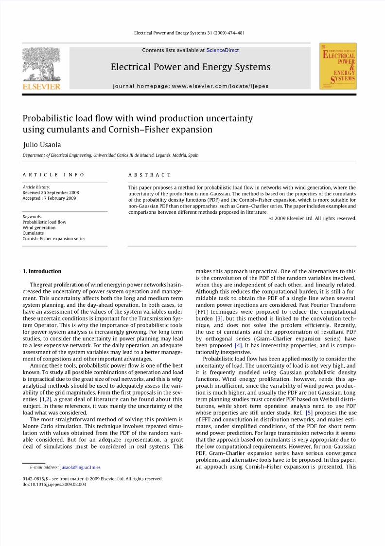
4.2. Computational procedure

The proposed method begins from a deterministic evaluation of line flows, using wind power predictions. Then, the probabilisticload flow follows, which provides the CDF of the lines of interest.It must be remarked that the deterministic prediction is the ex-pected value of the predicted power.

Hence, the following steps should be followed to find the CDF of the line flows.

1. Solve a DC load flow with the expected value of the wind powerinjected to the system. This gives the mean (expected value) of line power flows.

2. Calculate the moments and cumulants of the CDF of the windpower injections, using (4) and (12).

3. Use Eq. (15) to find the cumulants of the random variables of the power flows through the lines of interest. Coefficients aij

are obtained from Eq. (21).4. Use the Cornish–Fisher expansion (19) to find the value of the

CDF of the power in the lines of interest.

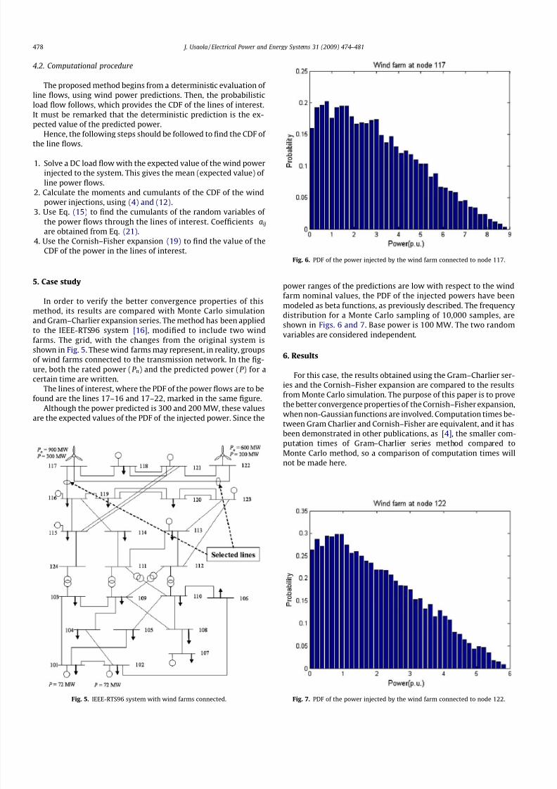
5. Case study

In order to verify the better convergence properties of thismethod, its results are compared with Monte Carlo simulationand Gram–Charlier expansion series. The method has been appliedto the IEEE-RTS96 system [16], modified to include two windfarms. The grid, with the changes from the original system isshown in Fig. 5. These wind farms may represent, in reality, groupsof wind farms connected to the transmission network. In the fig-ure, both the rated power (P n) and the predicted power (P ) for acertain time are written.

The lines of interest, where the PDF of the power flows are to befound are the lines 17–16 and 17–22, marked in the same figure.

Although the power predicted is 300 and 200 MW, these valuesare the expected values of the PDF of the injected power. Since the

power ranges of the predictions are low with respect to the windfarm nominal values, the PDF of the injected powers have beenmodeled as beta functions, as previously described. The frequencydistribution for a Monte Carlo sampling of 10,000 samples, areshown in Figs. 6 and 7. Base power is 100 MW. The two randomvariables are considered independent.

6. Results

For this case, the results obtained using the Gram–Charlier ser-ies and the Cornish–Fisher expansion are compared to the resultsfrom Monte Carlo simulation. The purpose of this paper is to provethe better convergence properties of the Cornish–Fisher expansion,

when non-Gaussian functions are involved. Computation times be-tween Gram Charlier and Cornish–Fisher are equivalent, and it hasbeen demonstrated in other publications, as [4], the smaller com-putation times of Gram–Charlier series method compared toMonte Carlo method, so a comparison of computation times willnot be made here.

Fig. 5. IEEE-RTS96 system with wind farms connected.

Fig. 6. PDF of the power injected by the wind farm connected to node 117.

Fig. 7. PDF of the power injected by the wind farm connected to node 122.




The number of Monte Carlo samples is 10,000. With this num-ber of samples there is a 95% probability that the greatest error inthe mean of the power in the considered branches is smaller than3.95%.

The method obtains a very good approximation to the momentsof power flows through lines. Let the error in the approximation of

the central moment of order n be defined in the following way:

en ¼ 1

N B

XN B j¼1

lann; j À lMC

n; j

lMC

n; j

Á 100

where lann; j is the central moment of order n of branch j found ana-

lytically, while lMC n; j is the same moment obtained by Monte Carlo

method. N B is the number of branches in the grid.Then, the value of this error for all the branches in the grid con-

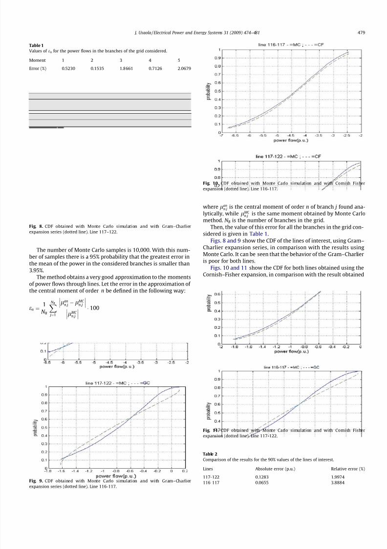
sidered is given in Table 1.Figs. 8 and 9 show the CDF of the lines of interest, using Gram–

Charlier expansion series, in comparison with the results usingMonte Carlo. It can be seen that the behavior of the Gram–Charlieris poor for both lines.

Figs. 10 and 11 show the CDF for both lines obtained using theCornish–Fisher expansion, in comparison with the result obtained

Fig. 10. CDF obtained with Monte Carlo simulation and with Cornish Fisherexpansion (dotted line). Line 116-117.

Table 1

Values of en for the power flows in the branches of the grid considered.

Moment 1 2 3 4 5

Error (%) 0.5230 0.1535 1.8661 0.7126 2.0679

Fig. 8. CDF obtained with Monte Carlo simulation and with Gram–Charlierexpansion series (dotted line). Line 117–122.

Fig. 9. CDF obtained with Monte Carlo simulation and with Gram–Charlierexpansion series (dotted line). Line 116-117.

Fig. 11. CDF obtained with Monte Carlo simulation and with Cornish Fisherexpansion (dotted line). Line 117-122.

Table 2

Comparison of the results for the 90% values of the lines of interest.

Lines Absolute error (p.u.) Relative error (%)

117-122 0.1283 1.9974

116-117 0.0655 3.8884




using Monte Carlo. It can be observed that the fitting in this case isvery good.

Another numerical comparison given here is the difference be-tween the values given by Monte Carlo method and Cornish–Fisherexpansion for a quantile of 90%. This is shown in Table 2.

The accuracy of these results allows to consider Cornish–Fisherexpansion more adequate for the problem conditions (non-Gauss-ian PDF of the wind power uncertainties), instead of theGram–Charlier expansion series. More examples have been runwith identical result. Only when the PDF of the injection powerare Gaussian, are the results comparable.

7. Conclusion

The operation of power systems with high wind power penetra-tion must consider the uncertainty of short term wind power pre-diction, and therefore new analysis tools must be used to deal withit. System Operators usually work with expected values for the in-

jected power, but due to the relatively low accuracy of the predic-tions, actual values may differ widely from those expected and thesystem variables may be also very different from those planned.

In relation with this problem, it has been shown that the Cor-nish–Fisher expansion represents an interesting method for per-forming probabilistic load flows in networks with wind power,where the PDF of the power injections are non Gaussian. Under

these conditions, other methods like Gram–Charlier series are lessadequate because of their worse convergence properties. Althoughthe convergence of Cornish–Fisher series have not been obtainedtheoretically, empirical results show that they fit better the non-Gaussian nature of the PDF involved.

The next developments of this work will be centered on themodeling of prediction uncertainty, the consideration of depen-dence between random variables and other ways of building theresulting PDF from the moments.

Acknowledgements

This research has been carried out within the research projectsAnemos Plus (6th FP European Project. Reference 38692) and IE-

MEL, Research Project of the Spanish Ministry of Education (Refer-ence ENE2006- 05192/ALT). Most of this work has been made

during a sabbatical leave from the Universidad Carlos III de Madridin the Ecole Superieure d’Electricité (Supélec), France. The stay hasbeen also financed by the Spanish Ministry of Education within theprogram ‘‘Estancias de profesores e investigadores españoles encentros de enseñanza superior e investigacion extranjeros” (Refer-ence PR2007-0032).

Appendix A. Tchebycheff–Hermite polynomials

A distribution u( x) that is N(0,1) can be written as

uð xÞ ¼ 1 ffiffiffiffiffiffiffi2p

p eÀ12 x2

If we call D ¼ ddx

, the successive derivatives with respect to x are:

Duð xÞ ¼ À xuð xÞD2uð xÞ ¼ ð x2 À 1Þuð xÞD3uð xÞ ¼ ð3 x À x3Þuð xÞ

The result will be a polynomial in x multiplied by u( x). We thendefine the Tchebycheff–Hermite polynomial H r ( x) by the identity

ðÀDÞr uð xÞ ¼ H r ð xÞuð xÞH r ( x) is of degree r in x and the coefficient of xr is unity. By conven-tion H 0 = 1, the following recurrence equation gives the value forr > 0.

H r ð xÞ ¼ xH r À1ð xÞ À ðr À 1ÞH r À2ð xÞThe polynomials have an important orthogonality property,

namely, thatZ 1

À1H mð xÞH nð xÞuð xÞdx ¼ 0 m–n

¼ n! m ¼ n

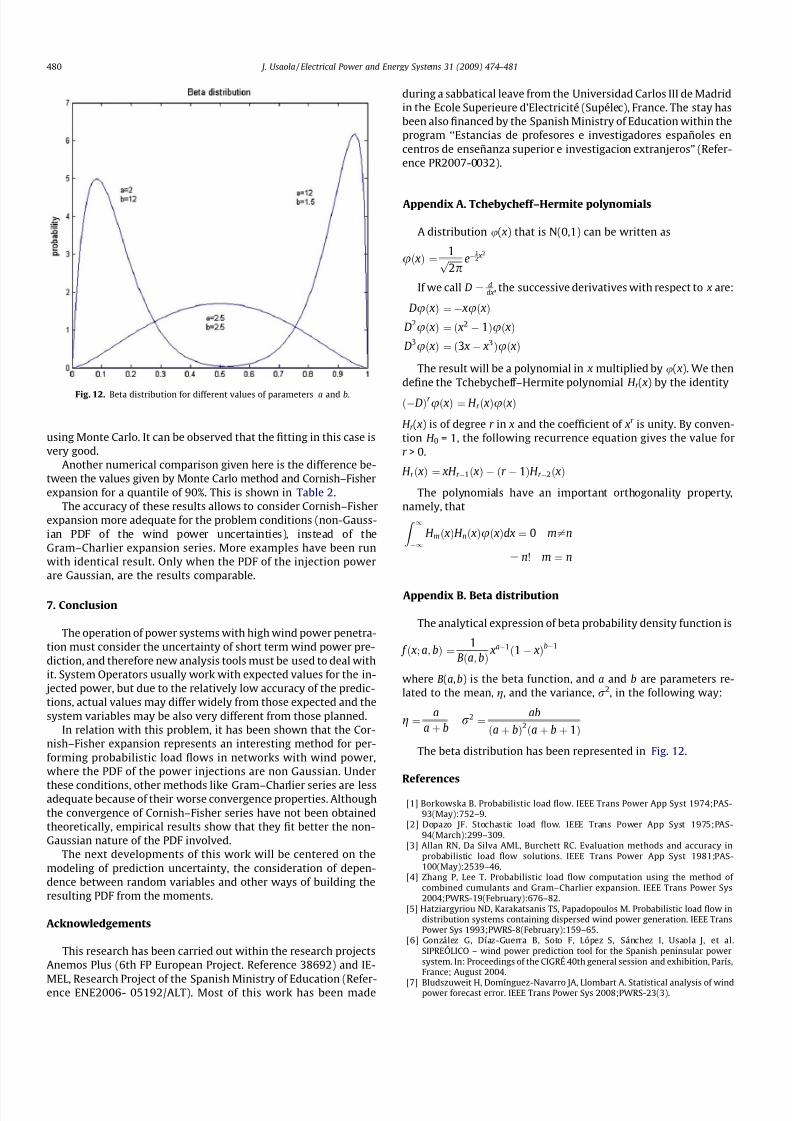
Appendix B. Beta distribution

The analytical expression of beta probability density function is

f ð x;a; bÞ ¼ 1

Bða;bÞ xaÀ1ð1À xÞbÀ1

where B(a, b) is the beta function, and a and b are parameters re-lated to the mean, g, and the variance, r2, in the following way:

g ¼ a

a þ br2 ¼ ab

ða þ bÞ2ða þ b þ 1ÞThe beta distribution has been represented in Fig. 12.

References

[1] Borkowska B. Probabilistic load flow. IEEE Trans Power App Syst 1974;PAS-93(May):752–9.

[2] Dopazo JF. Stochastic load flow. IEEE Trans Power App Syst 1975;PAS-94(March):299–309.

[3] Allan RN, Da Silva AML, Burchett RC. Evaluation methods and accuracy inprobabilistic load flow solutions. IEEE Trans Power App Syst 1981;PAS-100(May):2539–46.

[4] Zhang P, Lee T. Probabilistic load flow computation using the method of combined cumulants and Gram–Charlier expansion. IEEE Trans Power Sys2004;PWRS-19(February):676–82.

[5] Hatziargyriou ND, Karakatsanis TS, Papadopoulos M. Probabilistic load flow indistribution systems containing dispersed wind power generation. IEEE TransPower Sys 1993;PWRS-8(February):159–65.

[6] González G, Díaz-Guerra B, Soto F, López S, Sánchez I, Usaola J, et al.SIPREÓLICO – wind power prediction tool for the Spanish peninsular powersystem. In: Proceedings of the CIGRÉ 40th general session and exhibition, París,France; August 2004.

[7] Bludszuweit H, Domínguez-Navarro JA, Llombart A. Statistical analysis of windpower forecast error. IEEE Trans Power Sys 2008;PWRS-23(3).

Fig. 12. Beta distribution for different values of parameters a and b.




[8] Usaola, J, Angarita J. Bidding wind energy under uncertainty. In: Proceedings of the 2007 ICCEP, Capri, Italy; May 2007.

[9] Papoulis A, Pillai SU. Probability, random variables and stochasticprocesses. McGraw-Hill; 2002.

[10] McCullagh P. Tensor methods in statistics. London: Chapman and Hall; 1987.[11] Cramer H. Numerical methods of statistics. Princeton, NJ: Princeton University

Press; 1946.[12] Kendall MG, Stuart A. The advanced theory of statistics, vol. I. London: Charles

Griffin & Co. Ltd.; 1958.

[13] Blinnikov S, Moessner R. Expansions for nearly Gaussian distributions. AstronAstrophys Suppl Ser 1998;130:193–205.

[14] Cornish EA, Fisher RA. Moments and cumulants in the specification of distributions. Revue de l’Institut Internat de Statis 1937;4:307–20.

[15] S.R. Jaschke. The Cornish–Fisher-expansion in the context of delta-gamma-normal approximations. http://www.jaschke-net.de/papers/CoFi.pdf .Discussion Paper 54, Sonderforschungsbereich 373, Humboldt-Universität zuBerlin; 2001.

[16] IEEE APM Subcommittee. The IEEE reliability test system. IEEE Trans PowerSyst 1999;14(3):1010–18.


http://www.jaschke-net.de/papers/CoFi.pdf

http://www.jaschke-net.de/papers/CoFi.pdf

Documents

09_EPES_Probabilistic Load Flow With Wind Production Uncertainty