Embed Size (px)
Citation preview

1
Chepter-1
INTRODUCTION 1.1 PRIMER
Designing a combustion chamber for a gas turbine engine requires expensive testing with
much iteration. Previously, the designer relied primarily on the past experience, test results
and analysis based on empirical formulations to make the final design decisions. High
temperatures, pressures and flow rates in the combustor result in a flow field where
comprehensive experimental data are so expensive to obtain. Thus, Computational Fluid
Dynamics (CFD) is an attractive design tool, since it has the potential to explain the flow
physics inside the combustor. A numerical analysis can be used to reduce the number of
design iterations by providing an insight into the changes that a design parameter should
undergo regarding the characteristics of the flow.
CFD modeling of gas turbine combustors has recently become an important tool in the
combustor design process. For many years the combustion system was much less amenable to
theoretical treatment than other components of the gas turbine. Improving the prediction
capabilities and reliability of CFD methods will reduce the cycle time between idea and a
working product.
The work presents a 3D numerical simulation of a model gas turbine combustor a small,
annular type combustor. The entire flow field is modeled, from the compressor diffuser to
turbine inlet. The model includes the flare holes, the dome holes, primary holes, secondary
holes and dilution holes. An 18 deg sector of the combustor is modeled using Pro-E Wildfire
4.0.
In gas turbine combustor there exists a range of complex, interacting physical and chemical
phenomena, included are fuel spray atomization and vaporization, turbulent transport, finite-
rate chemistry of combustion and pollutant formation, radiation and particulate behavior. In
1980’s rigorous description of these phenomena are however, either not available or require
mathematical models which are too complex for computation, when taken together in the
context of multi-dimensional flows. Now a day the sophistication in the models is
continuously increasing with improvements in numerical methods, computer capabilities and
physical understanding.

2
The present work focuses on the problem of accurately predicting turbulent flow fields inside
the complex three-dimensional geometry of an annular type gas turbine combustor. The time
averaged Navier-Stokes (N-S) equations are solved, using the standard k-epsilon turbulence
model CFDesign10 is used for the present calculations.
1.2. BACKGROUND AND MOTIVATION Gas, or combustion, turbines were originally developed in the 18th century. The first patent
for a combustion turbine was issued to England’s John Barber in 1791. Patents for modern
versions of combustion turbines were awarded in the late 19th century to Franz Stolze and
Charles Curtis, however early versions of gas turbines were all impractical because the
power necessary to operate the compressors outweighed the amount of power generated by
the turbine. To attain positive efficiencies, engineers were making effort to increase
combustion and inlet temperatures beyond the maximum allowable turbine material
temperatures of the day. It was not until the middle of this century that gas turbines
developed into practical machines, primarily as jet engines. World War II military programs
use some prototype combustion turbine units that were the very first use of such type of
engine. The race for jet engines was encouraged by World War II and therefore included
huge government subsidization of initial R&D. The power generation from gas turbines was
emerge later from these military advances in technology. Germany’s Junkers and Great
Britain’s Rolls- Royce were the only companies successful enough to enter general
production with their engines during the war.2 Technology transfers began to take place as
early as 1941, when Great Britain began working with the US on turbine engines.
Engineering drawings were shared between England’s Power Jets Ltd. and America’s GE
Company during this period. American companies such as GE and Westinghouse began
development of gas turbines for land, sea and air use which would not prove deployable until
the end of the war. Other companies which were to emerge later in the combustion turbine
market, such as Solar Turbines (the “Solar” refers only to the name of the company, not the
source of energy) also emerged during the war by fabricating high temperature materials,
such as steel for airplane engine exhaust manifolds. The knowledge gained by manufacturers
during this time would help them manufacture other gas turbine products in the post war
period. After World War II, gas turbine R&D was spurred in some areas and stunted in
others. In an example of R&D expansion, the transfer of detailed turbine plans from Rolls-
Royce to Pratt & Whitney was made as a repayment to the US for its assistance to Great
Britain under the Lend- Lease agreement.3, 4 this allowed Pratt & Whitney, previously

3
specialists in reciprocating engines, to emerge as a strong developer of combustion turbines.
In contrast, German and Japanese companies were expressly barred from manufacturing gas
turbines. These companies were able to emerge later. For example, Siemens began recruiting
engineers and designers from the jet engine industry as soon as it was allowed; beginning in
1952.5 Most developments in the 1950s and 1960s were geared towards gas turbines for
aircraft use. R&D received a boost when turbofan engines were employed by commercial
aircraft as well as for military use. For example, GE and Pratt & Whitney engines were used
in early Boeing and Douglas commercial planes. This advance of combustion turbines into
the commercial aviation market, and in some cases the boat propulsion market, allowed
manufacturers to sustain their development efforts even though entrance into the base load
electric power generation market was not yet even on the horizon. Gas turbines also began to
emerge slowly in the peaking power generation market. Westinghouse and GE both began to
form power generation design groups independent of their aircraft engine designers.
Westinghouse would later exit the jet engine business in 1960 while keeping its stationary gas
turbine division. Among US turbine manufacturers, only GE was especially able to transfer
knowledge between its ongoing aircraft engine and power generation turbine businesses.
The early 1960s saw the beginning of gas turbine “packages” for power generation. This
occurred when GE and Westinghouse engineers were able to standardize (within their own
companies) designs for gas turbines. This technology marketing innovation took place for
two main reasons. First, in order to win over customers from traditional steam turbine or
reciprocating engine equipment, manufacturers found that they were more successful if they
offered fully-assembled packages, which included turbines, compressors, generators, and
auxiliary equipment. Second, this standardization allowed for multiple sales with little
redesign for each order, easing the engineering burden and lowering the costs of gas turbines.
The 1960’s also marked the introduction of cooling technologies to gas turbines. This
advance was the single most important breakthrough in gas turbine development since their
practical advent during World War II. The cooling involved the circulation of fluids through
and around turbine blades and vanes. These cooling advances were originally part of the
military turbojet R&D program, but began to diffuse into the power generation turbine
programs about five years later. Advances in cooling, along with continuing improvements in
turbine materials, allowed manufacturers to increase their firing and rotor inlet temperatures
and therefore improve efficiencies.
Although manufacturers were making great technological strides in gas turbine development,
it was not until the Great Northeast Blackout of 1965 that the US utility market truly awoke

4
to need for additional peaking generation capacity. This peaking is exactly what gas turbines
were good for; their fast startup times would allow generators to match periods of high
demand. Even though simple-cycle gas turbines of the day had dismal efficiencies (only
about 25%) compared to those of coal-fired plants, their ability to handle peak loads led to an
increase in demand and renewed R&D from manufacturers. The combustion turbine
capabilities of US utilities rose dramatically in the late 1960s and early 1970s in response to
this trend.
The three main components in a gas turbine engine are the compressor, combustor, and
turbine. The engine operates on the principle of the Brayton cycle, where compressed air is
mixed with fuel and burned in the combustor under constant pressure. The resulting high
temperature, high pressure gas is expanded through the turbine, forcing the turbine to rotate
and power the compressor through the connecting shaft. The Brayton cycle describes the
ideal performance of a gas turbine engine. The first law efficiency of the Brayton cycle is
dependent on pressure ratio only and, for improved efficiency, a high pressure ratio is
desired. High specific work performance is also important, and is dependent on temperature
ratio. As a result of this interdependence, both pressure and temperature ratios need to be
increased to achieve a high performance engine.
Higher combustion temperatures are needed to increase the power produced by a gas turbine
engine. The high combustion temperatures require exceptional performance of turbine
components, specifically the leading edge and end wall region of the first stage nozzle guide
vane. The ability of these vanes to withstand the harsh thermal conditions limits the power
that the engine is able to produce. Thus, the turbine effectively limits the maximum
combustion temperature. The challenges in maintaining turbine durability include providing
resistance to failure from thermal loads, fatigue due to variations in loading and thermal
stresses, and corrosion due to the harsh environment. Complex cooling systems are required
to combat the effects of the thermal loads both on the turbine vanes and on the combustor
liner. Designs of these cooling systems are complicated further due to the non-uniformity of
the gases within the combustor and the complex flow fields in the turbine.
The pitch wise pressure gradient created by the vanes, the inlet profile to the turbine can have
a considerable effect on the structure of the secondary flow field. Therefore, it is critical to
model realistic combustor exit flows and quantify their effect on the secondary flows. The
flow at the exit to a typical gas turbine combustor exhibits non-uniformities in temperature,

5
pressure and velocity in the pitch and span directions. This flow is set up by the geometry of
the combustor and the cooling scheme employed for protecting the combustor liner. Common
elements that contribute to the non-uniformities include swirlers, dilution jet injection, film
cooling and combustor liner convective cooling techniques that may include film-cooling
holes, slots, and impingement geometries.
Computational fluid dynamics (CFD) can serve as a great advantage in this area once
successful benchmarks against experimental results have been demonstrated. Many
computational cases can be computed and analyzed in a relatively short period of time in
order to study various combustor designs, exit profiles, and their effect on the secondary
flows. Turbine inlet profiles can be tailored through the design of the combustor to minimize
secondary flows in the end wall region and minimize heat transfer. Ultimately, this would
allow higher temperatures to be reached and more power to be produced by the engine.
1.3. OBJECTIVES OF THE RESEARCH
The objective of this research is to analyses the cold flow performance of a combustion
chamber using computational fluid dynamics software. This is done by:
1. Understanding the work concept of gas turbine combustion chamber.
2. Familiarizing and applying the use of ProE Wildfire 4.0 Software for simulation purpose.
3. Familiarizing and applying the use of CFDesign10 & ANSYS softwares for analysis
purpose.
4. Simulate the model of gas turbine combustion chamber to
4.2.1. Estimate the mass distribution at different region with varying hole size
4.2.2. Estimate the total pressure drop at different region with varying hole size
1.4. SCOPE OF THE RESEARCH
The flow inside the gas turbine combustor is highly complex and major design requirements
depend to greater extent on the internal aerodynamics. The mixing as well as combustion
process in a gas turbine combustor is mainly influenced by the flow pattern, recirculation, jet

6
mixing, jet penetration and the turbulence. The research work may further be implemented
for analyzing the similar nature type of problem.
Preset study deals with the implementation of CFD for three-dimensional analysis of flow in
an annular gas turbine combustor. CFDesign10 has been used for the analysis, which includes
cold flow analysis. It will provide the mass distribution in each zone and the pressure drop
across the combustor. These informations will be useful to analyses the combustion products.
1.5 GAS TURBINE
Atmospheric air is utilized in gas turbine combustion system to produce the necessary power
and thrust. Gas turbines usually operate on an open cycle, as shown in fig. 1.1.
Fig. 1.1 (a) Operation of Open Cycle For Gas Turbine

7
Fig. 1.1 (b) P-V Curve of open cycle for gas turbine
Fig. 1.1(c) T-S curve and operation of open cycle for gas turbine
In an ideal gas turbine cycle i.e. Brayton cycle or reversed Jules cycle, fresh air at ambient
conditions (1) is drawn into the compressor as shown in the above fig.1.1, Air entering the
compressor at point 1 is compressed to some higher pressure. No heat is added; however,
compression raises the air temperature so that the air at the discharge of the compressor is at a

8
higher temperature and pressure (2). The high-pressure air proceeds into the combustion
chamber, where the fuel is burnt at constant pressure up to (3). The resulting high-
temperature gases then enter the turbine, where they expand to the atmospheric pressure (4 in
P-V diagram) through the nozzle vanes. This expansion causes the turbine blade to spin.
Again the expansion of gases is isentropic.
Combustion is the chemical process or a chemical change, especially oxidation, accompanied
by the production of heat and light. The function of the combustion chamber is (1) to accept
the air from the compressor at condition (2) and to deliver it to the turbine at the required
temperature on condition (3), ideally with no loss of pressure. Essentially it is a direct-fired
air heater in which fuel is burnt with less than one third of the air after which the combustion
products are then mixed with the remaining air.
In gas turbine the combustor is a critical component because it must operate reliably at
extreme temperatures and should provide a suitable temperature distribution at entry to
turbine and create the minimum amount of pollutants over a long operating life. Gas Turbine
performance is affected by following factors
Air Temperature and Site Elevation Humidity
Inlet and Exhaust Losses
Fuels
Fuel Heating
Diluent Injection
Air Extraction
Performance Enhancements
Inlet Cooling
Steam and Water Injection for Power Augmentation
Peak Rating
Combined cycle in its simplest form is shown in the Fig. No. Combined cycles producing
only electrical power are in the 50% to 60% thermal efficiency range using the more
advanced gas turbines.

9
Fig. 1.2. Combined cycles for gas turbine
High utilization of the fuel input to the gas turbine can be achieved with some of the more
complex heat-recovery cycles, involving multiple-pressure boilers, extraction or topping
steam turbines, and avoidance of steam flow to a condenser to preserve the latent heat
content. Attaining more than 80% utilization of the fuel input by a combination of electrical
power generation and process heat is not unusual Combined cycles producing only electrical
power are in the 50% to 60% thermal efficiency range using the more advanced gas turbines.
1.6. COMBUSTOR 1.6.1. Outline
The combustor is the part where energy is inserted into the gas turbine. The combustor
section of simple- and combined-cycle gas turbines can be thought of as the heart of the
system. Proper combustor design and operation are critical for establishing maximum unit
performance.The choice of a particular combustor type and layout is determined largely by
the overall engine design and by the need to use the available space as effectively as possible.
There are two basic types of gas turbine combustors, tubular and annular. A compromise
between these two extremes is the “tuboannular” combustor, in which a number of equi
spaced tubular liners are placed within an annular air casing. The three different combustor
types are shown in fig. 1.3.

10
multitubular combustor tuboannular combustor annular combustor
Fig.1.3. Diagram showing layout of combustor types
A tubular combustor fig. 1.4 composed of a cylindrical liner mounted concentrically inside a
cylindrical casing. Most of the early jet engines featured tubular chambers, usually in
numbers varying from seven to sixteen per engine. Nowadays the tubular combustor is used
mainly for small gas turbine of low power out.
Fig. 1.4.Diagram showing tubular combustor
The annular combustors fig. 1.4 comprises an annular liner mounted concentrically inside an
annular casing. It represents an ideal configuration in terms of compact units of lower
pressure lose than other combustor types. Annular combustors, offer maximum utilization of
available volume, fewer requirements of cooling air and high temperature application. A well
designed gas turbine combustor should have complete combustion and minimal total pressure

11
loss over a wide range of operating conditions. Flow characteristics in the annulus passage
surrounding the liner is equally important as the flow is fed into the liner through the annulus
passage.
Unfortunately, annular combustors presents serious difficulties, firstly, although a large
number of fuel jets can be employed, it is more difficult to obtain an even fuel/air distribution
and an even outlet temperature distribution. Secondly, the annular chamber is inevitably
weaker in structure and it is difficult to avoid buckling of the hot flame tube walls. Thirdly,
most of the development work must be carried out on the complete combustion chamber,
requiring a test facility capable of supplying the full engine air mass flow.
Fig.1.5. Diagram showing annular combustor
The tuboannular combustor, a group of cylindrical liners is arranged inside a single annular
casing, as illustrated in fig. 1.5 this type represents an attempt to combine the compactness of
the annular combustor with the best features of the tubular system. A drawback to the
tuboannular combustor, which it shares with tubular configuration, is the need for
interconnectors. Compared with the annular design, the tuboannular combustor has an
important advantage in that much useful chamber development can be carried out with
modest air supplies, using just a small segment of chamber containing one or more liners.
Tuboannular chambers are still in widespread use, although the great majority of modern
combustors for large engines are of annular form.

12
Fig. 1.6. Diagram showing tuboannular combustor
1.6.2. Combustor Requirements
A gas turbine combustor must satisfy a wide range of requirements whose relative
importance varies among engine types. However, the basic requirements of all combustors
are as follows:
a. High combustion efficiency (i.e., the fuel should be completely burned so that its all
chemical energy is liberated as heat).
b. Reliable and smooth ignition both on the ground (especially at very low ambient
temperatures) and in the case of aircraft engines after a flame out at high altitude.
c. Wide stability limits (i.e., the flame should stay alight over wide range of pressure and
air-fuel ratio).
d. Low pressure loss
e. Low emission of gaseous and smoke pollutant species.
f. A satisfactory outlet temperature distribution tailored to the demands of the turbine.
g. Freedom from pressure pulsations.
h. Minimum manufacturing cost, size, and weight for the particular application.
i. Long operating life.

13
j. Ease of maintenance.
k. Multifuel capability.
The priority given to each of the above requirements will vary with the intended engine
application.
1.6.3. Main Parts of Gas Turbine Combustor
The following are the important components of the gas turbine combustor:
a. Diffuser
b. Swirler
c. Fuel Injector
d. Spark Plug
e. Liner
f. Casing
Fig.1.7. Diagram showing main parts of gas turbine combustor

14
1.6.3.1. Diffuser
In axial-flow compressor the stage pressure is very dependent on the axial flow velocity. To
achieve the design pressure ratio in the minimum number of stages, a high axial velocity is
essential in many aircraft engines, compressor outlet reaches 170m/s or higher. It is of course,
impracticable to attempt to burn the fuel in air flowing at such higher velocities. Quite apart
from the formidable combustion problems involved, the fundamental pressure loss would be
excessive. Thus before combustion can proceed, the air velocity must be greatly reduced,
usually to about one-fifth of the compressor outlet velocity. This reduction in velocity is
achieved by fitting a diffuser between the compressor outlet and the upstream end of the
liner.
In its simplest form, a diffuser is merely a diverging passage in which the flow is decelerating
and the reduction in velocity head is converted to rise in static pressure. The efficiency of this
conversion process is of considerable importance because any losses that occur are
manifested as a fall in total pressure across the diffuser.
An ideal diffuser is one that achieves the required velocity reductions in the shortest possible
length with minimum total pressure loss and uniform flow conditions. There are mainly two
philosophies in regarded to diffuser design. One is to employ a relatively long aerodynamics
diffuser to achieve maximum recovery of dynamic pressure. The other is based on the use of
a short annular diffuser immediately down streams of the compressor outlet, followed by
sudden expansion. Compared to an aerodynamic diffuser, dump diffuser is shorter in length
and is reputed to be less sensitive to variations in compressor outlet velocity profile. Its
obvious disadvantages are a higher-pressure loss and low static pressure across the dome.
1.6.3.2. Swirler
It is located at the entrance of the liner. The function of the swirler is to provide a swirling
motion to the air coming out of the diffuser. Here the axial velocity is converted to
circumferential velocity.
Swirling action is essential in order to mix thoroughly the air and the injected fuel i.e., to
obtain improved turbulence, as to ensure the complete combustion of fuel and thereby
increasing the thermal efficiency. There are several factors influencing the size of the
recirculation zone downstream of the Swirler. The size of the recirculation zone is increased
by increase in the vane angle, an increase in number of vanes i.e., a decrease in vane aspect

15
ratio and changing from the flat to curved vane. The amount of rotations imparted to axial
flows is given by non-dimensional number i.e. Swirl number (Sn). For values of Sn less than
around 0.4, no flow circulation is obtained and swirl is weak. When streamlines diverge,
swirl is moderate. This region corresponds to Sn between 0.4 - 0.6. If Sn = 0.6 it is strong
Swirl and most of the Swirlers operate at this condition.
1.6.3.3. Fuel Injector
It is used for the purpose of atomization of fuel. Fuel is introduced by various techniques
such as pressure atomizing, air blast atomizing, vaporizing and premix/pre-vaporizing.
Pressure atomizers are relatively simple in construction. Provide a wide flow range and can
provide good fuel atomization when fuel system pressures are high.
In air blast atomizer by means of gas dynamics shear forces generated by strong swirling
motion accompanied by counter swirl, liquid fuel is atomized, in vaporizing technique the
fuel and air are introduced into a cone shaped tube immersed in combustion zone. During
operation, heat transfer from the combustion chamber partially vaporizes the incoming fuel,
while the liquid / vapor fuel within the tube provides thermal protection for the tube. In
premixing technique, fuel is introduced and premixed with the incoming air prior to the
introduction into the combustion zone. This provides a uniform, fully mixed field of
vaporized fuel in the combustion region. This results in low smoke and chemical emissions
and improves fuel air uniformity in combustion zone.
1.6.3.4. Spark Plug
The function of spark plug or the igniter plug is to generate spark for ignition of air fuel
mixture. The mode of ignition is by means of electrical discharge such as spark or arc
discharge. Spark discharges convert electrical fairly efficiently into heat that is concentrated
in a relatively small volume.
1.6.3.5. Liner
The function of the liner or the flame tube is to provide a region of low velocity in which
combustion is sustained by a recirculatory flow of burnt products that provide a continuous
source of ignition for incoming fuel mixture.
1.6.3.6. Casing

16
The casing is the outer container of the combustor. It is the structural shell that carries the
thrust loads. In this case of an annular combustor, there is a single casing which covers all the
flame tubes as opposed to the tubular type which has individual casing for each of the flame
tubes. This type of arrangement in an annular combustor drastically reduces the weight of the
engine.
1.6.3.7. Primary Zone
The purpose of the primary zone is to anchor the flame and, at the same time, provide
sufficient time, temperature, and turbulence to achieve essentially complete combustion of
the fuel. An essential feature is the toroidal flow reversal that is created and maintained by air
entering trough swirl vanes located around the fuel injector and through a single row of holes
in the wall of the liner. This flow reversal ensures that some of the hot gases produced in
combustion are recirculated back into the primary zone to mix with the incoming air and fuel.
1.6.3.8. Intermediate or Secondary Zone
The secondary zone is the region that lies between the primary and dilution zones as shown in
fig. 1.6. At low combustion pressures, the rate of chemical reaction is slow and the
combustion is far from complete at exit from the primary zone. Under these conditions the
intermediate zone serves principally as an extension to the primary zone, providing increased
residence time for combustion to proceed to completion. At high combustion pressures the
intermediate zone serves a different purpose. Although high pressures ensure complete
combustion, at the high temperatures prevailing in the primary zone, dissociation of carbon
dioxide to carbon monoxide and oxygen occurs and, to a lesser extent, dissociation of water
vapor to hydrogen and oxygen. Lowering the flame temperature, by injecting prudent
amounts of air into the secondary zone, inhibits dissociation and allows the combustion of
carbon monoxide and hydrogen to proceed to completion upstream of the dilution zone.
1.6.3.9. Dilution Zone
The role of the dilution zone is to admit the air remaining after the combustion and wall-
cooling requirements have been met, and to provide an outlet stream with a mean temperature
and a temperature distribution that are acceptable to the turbine. The dilution air is introduced
through one or more rows of holes in the airs liner walls. [3][17]

17
1.6.4. Combustion Process
The combustion in gas turbine combustors takes place in three zones viz. primary,
intermediate or secondary and dilution zones. In a combustor the flame is stabilized by
recirculation of hot combustion products. This means that the fresh combustibles are vitiated
by the burned products at the instant of ignition. Thus, the rates of combustion (and stability)
are influenced by a tradeoff between temperature rise and limitation necessitating a
successful compromise. Fig. 1.6 shows combustion zones in combustion chamber.
Gas turbines mainly use kerosene-type fuels. These fuels consist of hydrocarbons with the
chemical composition CxHy. They are mixed with air and then combusted. The ideal reaction
is then given by
CxHy + ε(XO2O2 + XN2N2 + XCO2CO2 + XArAr)→ nCO2CO2 + nH2OH2O + nN2N2 + nArAr.
In this equation, the X’s indicate the composition of air. We thus have
XO2 = 0.2095, XN2 = 0.7808, XCO2 = 0.0003 and XAr = 0.0094
The term ε is the number of moles of air necessary for every mole of fuel. It is given by
ε=( x+y/4) / XO2
Finally, the n,s denote the amount of reaction products. We find that we have
nCO2 = x + εXCO2 , nH2O = y/2, nN2 = εXN2 and nAr = εXAr .
In reality, we don’t have this ideal reaction. In the real world, not all fuel gets combusted. Not
all carbon atoms form carbon dioxide CO2. (We will also have carbon monoxide CO.) And
there will be various other reaction products as well. We won’t examine all those reaction
products though.
1.7 CFD (COMPUTATIONAL FLUID DYNAMICS) Fluid (gas and liquid) flows are governed by partial differential equations (PDE) which
represent conservation laws for the mass, momentum, and energy. Computational Fluid
Dynamics (CFD) is the art of replacing such PDE systems by a set of algebraic equations
which can be solved using digital computers. The object under study is also represented
computationally in an approximate discretized form. The physical aspects of any fluid flow
are governed by the following three fundamental principles: (1) mass is conserved; (2) F =
ma (Newton’s second law); and (3) energy is conserved. These fundamental principles can be
expressed in terms of mathematical equations, which in their most general form are usually
partial differential equations. Computational fluid dynamics is, in part, the art of replacing the
governing partial differential equations of fluid flow with numbers, and advancing these

18
numbers in space and/or time to obtain a final numerical description of the complete flow
field of interest. This is not an all-inclusive definition of CFD; there are some problems
which allow the immediate solution of the flow field without advancing in time or space, and
there are some applications which involve integral equations rather than partial differential
equations. In any event, all such problems involve the manipulation of, and the solution for,
numbers. The end product of CFD is indeed a collection of numbers, in contrast to a closed-
form analytical solution. However, in the long run the objective of most engineering analyses,
closed form or otherwise, is a quantitative description of the problem, i.e. numbers. (See, for
example, Ref. [4]). Of course, the instrument which has allowed the practical growth of CFD
is the high-speed digital computer. CFD solutions generally require the repetitive
manipulation of thousands, or even millions, of numbers—a task that is humanly impossible
without the aid of a computer. Therefore, advances in CFD, and its application to problems of
more and more detail and sophistication, are intimately related to advances in computer
hardware, particularly in regard to storage and execution speed. This is why the strongest
force driving the development of new super computers is coming from the CFD community
(see, for example, the survey article by Graves [5]).
1.7.1. Numerical Discretization Technique
In this process of numerical discretization each term within a partial differential equation is
translated into a numerical analogue that the computer can be programmed to calculate.
Some of the numerical discretization techniques are:
a. Finite Difference Method
b. Finite Element Method
c. Finite Volume Method
1.7.2. Finite Element Method
Finite element methods are extensively used in engineering because of their versatility in the
solution of a wide range of practical problems. In our present study we use finite element
method for discretization. Finite difference methods are generally easier to understand and
apply, as compared to finite element methods; they also have smaller memory and
computational time requirements.

19
Thus, these are easier to develop and to program. However, practical problems generally
involve complicated geometries, complex boundary conditions, material property variations,
and coupling between different domains. Finite element methods are particularly well suited
for such circumstances because they have the flexibility to handle arbitrary variations in
boundaries and properties. Consequently, much of the software developed for engineering
systems and processes in the last two decades has been based on the finite element method
(Huebner and Thornton, 2001; Reddy, 2004). Available software is used extensively in finite
element solutions of engineering problems because of the tremendous effort generally needed
for the development of the computer program. [18]
The finite element method originated from the need for solving complex elasticity and
structural analysis problems in civil and aeronautical engineering. Its development can be
traced back to the work by Alexander Hrennikoff (1941) and Richard Courant (1942). While
the approaches used by these pioneers are dramatically different, they share one essential
characteristic: mesh discretization of a continuous domain into a set of discrete sub-domains,
usually called elements.
Hrennikoff's work discretizes the domain by using a lattice analogy while Courant's approach
divides the domain into finite triangular subregions for solution of second order elliptic
partial differential equations (PDEs) that arise from the problem of torsion of a cylinder. The
finite element method (FEM) (its practical application often known as finite element analysis
(FEA)) is a numerical technique for finding approximate solutions of partial differential
equations (PDE) as well as of integral equations. The solution approach is based either on
eliminating the differential equation completely (steady state problems), or rendering the
PDE into an approximating system of ordinary differential equations, which are then
numerically integrated using standard techniques such as Euler's method, Runge-Kutta, etc.
In solving partial differential equations, the primary challenge is to create an equation that
approximates the equation to be studied, but is numerically stable, meaning that errors in the
input and intermediate calculations do not accumulate and cause the resulting output to be
meaningless. There are many ways of doing this, all with advantages and disadvantages. The
finite element method is a good choice for solving partial differential equations over
complicated domains (like cars and oil pipelines), when the domain changes (as during a
solid state reaction with a moving boundary), when the desired precision varies over the
entire domain, or when the solution lacks smoothness.

20
The finite element method is based on the integral formulation of the conservation principles.
The computational domain is divided into a number of finite elements, several types and
forms of which are available for different geometries and governing equations. The complete
system may be complex and irregularly shaped, but the individual elements are easy to
analyze. The elements may be one dimensional (1-D), two dimensional (2-D) (triangular or
quadrilateral), or three dimensional (3-D) (tetrahedral, hexahedral, etc.) as shown in fig. 1.8;
and may be linear or higher-order.
Fig.1.8. Diagram showing 1-D, 2-D and 3-D elements
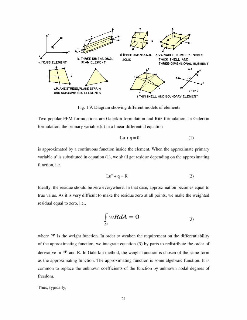
The elements may model mechanics, acoustics, thermal fields, electromagnetic fields, etc., or
coupled problems. In a mechanical problem, the elements may model membranes, beams,
thin plates, thick plates, solids, fluids, etc. as shown in fig.1.9.
The variation of the dependent variable is generally taken as a polynomial and frequently as
linear within the elements. Integral equations that apply for each element are derived and the
conservation principles are satisfied by minimization of the integrals or by reducing their
residuals to zero. [19][20][21]
21
Fig. 1.9. Diagram showing different models of elements
Two popular FEM formulations are Galerkin formulation and Ritz formulation. In Galerkin
formulation, the primary variable (u) in a linear differential equation
Lu + q = 0 (1)
is approximated by a continuous function inside the element. When the approximate primary
variable ue is substituted in equation (1), we shall get residue depending on the approximating
function, i.e.
Lue + q = R (2)
Ideally, the residue should be zero everywhere. In that case, approximation becomes equal to
true value. As it is very difficult to make the residue zero at all points, we make the weighted
residual equal to zero, i.e.,
D
wRdA 0 (3)
where is the weight function. In order to weaken the requirement on the differentiability
of the approximating function, we integrate equation (3) by parts to redistribute the order of
derivative in and R. In Galerkin method, the weight function is chosen of the same form
as the approximating function. The approximating function is some algebraic function. It is
common to replace the unknown coefficients of the function by unknown nodal degrees of
freedom.
Thus, typically,

22
ue = [N]{une} (4)
where [N] is the matrix of shape functions and {une} is the nodal degrees of freedom. In Ritz
formulation, the differential equation (1) is converted into an integral form using calculus of
variation. The approximation (equation (4)) is substituted in the integral form and the form is
extremized by partially differentiating with respect to {une}.
After obtaining the elemental equations, the assembly is performed. A simple way of
assembly is to write equations for each element in global form and then add each similar
equations of all the elements, i.e., we add the equation number 1 from each element to obtain
the first global equation, all equation number 2 are added together to give second equation,
and so on. The boundary conditions are applied to assembled equation and then are solved by
a suitable solver. Then, post-processing is carried out to obtain the derivatives. [22]
1.7.3. Governing Equations
The governing equations are the mathematical statements of three fundamental physical
principles upon which all of fluid dynamics is based.
a. Mass is conserved
b. Newton’s second law
c. Energy is conserved
When the above three physical principles are applied to the considered model of flow, we can
derive the governing equations of fluid flow. When the principle of mass conservation is
applied to the model of flow we arrive at the equation called as Continuity equation. When
Newton’s second law is applied to the model of flow we arrive at the set of equations called
as Momentum equations. When the principle of energy conservation is applied to the
considered model of flow, we arrive at Energy equation. The above three equations are
called as the Governing equations of the fluid dynamics. The governing equations for the
unsteady, compressible, three-dimensional, viscous flow in conservation form are as follows:
1.7.4. Continuity equation
The equation for mass conservation or continuity equation for viscous flow is given by
0).( Vt
(4.3.1)

23
where ρ is the fluid density and V is fluid velocity given by
wkvjuiV
1.7.5. Momentum equations
The equation for the Newton’s second law or momentum equations for viscous flow are
given by
ut
uVpx x y z
f
vt
vVpy x y z
f
wt
wVpz x y z
f
xx yx zx
x
xy yy zy
y
xz yz zz
z
.
.
.
(4.3.2)
1.7.6. Energy equation
The equation for the principle of energy conservation or Energy equation for viscous flow is
given by
t
eV
eV
V qx
kTx y
kTy z
kTz
2 2
2 2.
upx
vpy
wpz
ux
u
yu
z
v
x
v
yxx yx zx xy yy
v
zw
x
w
yw
zf Vzy xz yz zz . (4.3.3)
where the shear stresses are given by

24
xx
yy
zz
xy yx
xz zx
zy yz
Vux
Vvy
Vwz
vx
uy
wx
uz
vz
wy
.
.
.
2
2
2
(4.3.4(a))
and operator is given by
x
iy
jz
k (4.3.4(b))
These equations are the coupled system of non-linear partial differential equations and hence
are very difficult to solve analytically. There is no general closed form solution to these
equations. So there must be some other method followed in order to solve these equations.
One best possible method is the numerical method. Numerical method coupled with the
computational technique increases the solving speed of these equations. CFD codes are
developed in order to solve these equations. There are a lot of CFD codes commercially
available. [23]
1.7.7. Turbulence Models
Turbulence is a natural phenomenon in fluids. Significant variations in the velocity field,
irregularity in both space and time are the essential feature of turbulent flows. An important
characteristic of turbulence is its ability to mix fluid much more effectively than a
comparable laminar flow. Reynolds established that flow is characterized by single non-
dimensional parameter, known as Reynolds number (Re). It is defined by ratio of inertia force
to viscous force,
Re
UL (4.4)

25
where U and L are characteristic velocity and length scale respectively, and is kinematic
viscosity. At low Reynolds number inertia forces are smaller than the viscous forces. The
naturally occurring disturbances are dissipated away and the flow remains laminar. At high
Reynolds number, the inertia forces are sufficiently large to amplify the disturbances and a
transition to turbulence occurs. Here, the motion becomes intrinsically unstable even with
constant imposed boundary condition. The velocity and all other properties are varying in a
random and chaotic way.
Turbulent fluctuations always have a 3D spatial character. Visualization of turbulent flows
have revealed rotational flow structures, so called turbulent eddies, with a wide range of
length and velocity scales called turbulent scales. The largest eddies have a characteristic
velocity and characteristic length of the same order as the velocity and length scale of the
mean flow. For turbulent flows, where UL >> ν the largest eddies whose scale are
comparable with mean flow, are dominated by inertia effects rather than viscous effects.
Transport of eddies is attained by extraction of energy from the mean flow by a process
called vortex stretching. The presence of velocity gradients in the mean flow causes
deformation of the fluid such as, shear and linear strain and rotation, which “stretch” eddies
that are appropriately aligned by forcing one end of the eddies to move faster than the other.
During vortex stretching the angular momentum is conserved and the stretching work done
by the mean flow on the large eddies provides the energy that maintains the turbulence. This
large eddy than breed new instabilities creating smaller eddies, which are transported mainly
by vortex stretching. Thus, the energy is handed over from the large eddy to the smaller eddy.
This process continues until the eddies become so small that viscous effect become
important.
In direct numerical simulation (DNS), a refined mesh is used so that all of these scales, large
and small, are resolved. This is known as the deterministic method. Although some simple
problems have been solved using DNS, it is not possible to undertake industrial problems of
practical interest due to the prohibitive computer cost. Since turbulence is characterized by
random fluctuations, statistical methods rather than deterministic methods have been studied
extensively in the past. In this approach, time averaging of variables is carried out in order to
separate the mean quantities from fluctuations, this result in new unknown variable(s)
appearing in the governing equations. Thus, additional equation(s) are introduced to close the
system, the process known as turbulence modeling or Reynolds averaged Navier-Stokes

26
(RANS) methods. In this approach, all large and small scales of turbulence are modeled so
that mesh refinements needed for DNS are not required.
Turbulent flows are characterized by fluctuating velocity fields. These fluctuations mix
transported quantities such as momentum, energy, and species concentration, and cause the
transported quantities to fluctuate as well. Since these fluctuations can be of small scale and
high frequency, they are too computationally expensive to simulate directly in practical
engineering calculations. Instead, the instantaneous (exact) governing equations can be time-
averaged or otherwise manipulated to remove the small scales, resulting in a modified set of
equations that are computationally less expensive to solve. [23][24]
1.8. OVERVIEW OF SOFTWARE DETAILS Softwares are the important part of this research work. These softwares are very effective in
time and cost saving tools for generating geometry and analyzing the problem indifferent
condition. ProE is used for the drawing the geometry, Gambit is used for the meshing the
geometry and defining the initial boundary condition and then the problem is exported to
Fluent for estimating the desired result. A brief introduction of different software used is
given in the next section.
1.8.1. Pro/ENGINEER (ProE)
Pro/ENGINEER (ProE) is a drawing tool developed by Product Development Company for
making drawing in 2D/3D with smart application of different modules. ProE not only lets
you design individual parts quickly, it also records their assembly relationships and produces
finished mechanical drawings. There are three basic ProE design modules from conception
to completion. Each design step is treated as a separate ProE mode, with its own
characteristics, file extensions, and relations with the other modes.
Pro/ENGINEER Wildfire 4.0 is a powerful program used to create complex designs with a
great precision. The design intent of any three-dimensional (3D) model or an assembly is
defined by its specification and its use. You can use the powerful tools of Pro/ENGINEER
Wildfire 4.0 to capture the design intent of any complex model by incorporating intelligence
into the design. To make the designing process simple and quick, this software package has
divided the steps of designing into different modules. This means that each step of designing
27
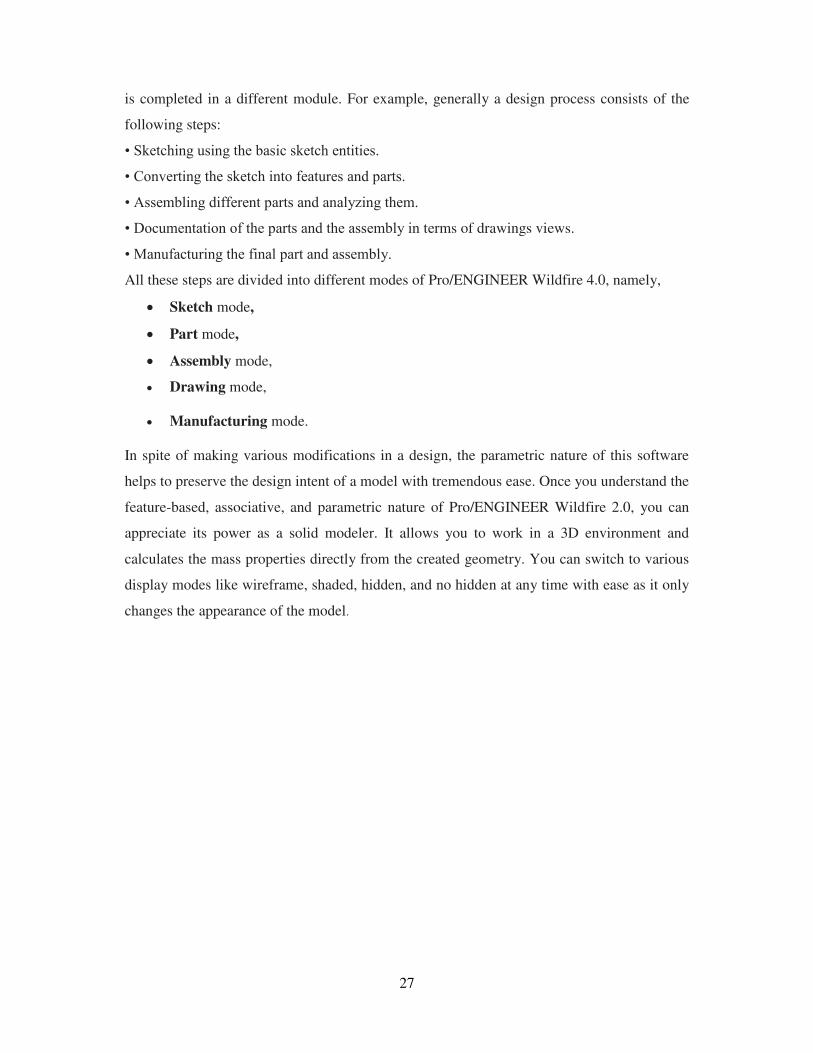
is completed in a different module. For example, generally a design process consists of the
following steps:
• Sketching using the basic sketch entities.
• Converting the sketch into features and parts.
• Assembling different parts and analyzing them.
• Documentation of the parts and the assembly in terms of drawings views.
• Manufacturing the final part and assembly.
All these steps are divided into different modes of Pro/ENGINEER Wildfire 4.0, namely,
Sketch mode,
Part mode,
Assembly mode,
Drawing mode,
Manufacturing mode. In spite of making various modifications in a design, the parametric nature of this software
helps to preserve the design intent of a model with tremendous ease. Once you understand the
feature-based, associative, and parametric nature of Pro/ENGINEER Wildfire 2.0, you can
appreciate its power as a solid modeler. It allows you to work in a 3D environment and
calculates the mass properties directly from the created geometry. You can switch to various
display modes like wireframe, shaded, hidden, and no hidden at any time with ease as it only
changes the appearance of the model.

28
Figure 1.10. Items on the main window
The major advantages of using ProE are listed below
Very quick in creating the high quality and most innovative products drawing.
Fast-track concept design with free style design features
Increase productivity with more efficient and flexible 3D detailed design capabilities.
Increase model quality, promote native and multi-CAD part reuse, and reduce model
errors.
Handle complex surfacing requirements with ease.
1.8.1.1.PARAMETRIC NATURE OF Pro/ENGINEER WILDFIRE 4.0 Pro/ENGINEER Wildfire 4.0 is parametric in nature, which means that the features of a part
become interrelated if they are drawn by taking the reference of each other. We can redefine
the dimensions or the attributes of a feature at any time. The changes will propagate
automatically throughout the model. Thus, they develop a relationship among themselves.
This relationship is known as the parent-child relationship. So if you want to change the

29
placement of the child feature, you can make alterations in the dimensions of the references
and hence change the design as per your requirement
1.8.1.2. IMPORTANT TERMS AND DEFINITIONS
Some important terms that will be used, while working with Pro/ENGINEER Wildfire 4.0 are
discussed in this section
Weak Dimensions and Weak Constraints Weak dimensions and weak constraints are temporary dimensions or constraints that appear
in gray color. These are automatically applied to the sketch when it is drawn using the Intent
Manager. They are removed from the sketch without any confirmation from the user. The
weak dimensions or the weak constraints should be changed to strong dimensions or
constraints if they seem to be useful for the sketch. This only saves an extra step of
dimensioning the sketch or applying constraints to the sketch.
Strong Dimensions and Strong Constraints Strong dimensions and strong constraints appear in yellow color. These dimensions and
constraints are neither removed automatically nor applied automatically. All dimensions
added manually to a sketch are strong dimensions.
FILE MENU OPTIONS The options that are displayed when you choose File from the menu bar are discussed next. Working Directory A working directory is a directory on your system where you can save the work done in the
current session of Pro/ENGINEER Wildfire 4.0. You can set any directory existing on your
system as the working directory. Before starting work in Pro/ENGINEER Wildfire 4.0, it is
important to specify the working directory. If the working directory is not selected before
saving an object file then the object file will be saved in a default directory. This default
directory is set at the time of installing Pro/ENGINEER Wildfire 4.0. If the working directory
is selected before saving the object files that you create, it becomes easy to organize them. In
Pro/ENGINEER Wildfire 4.0, the working directory can be set in two ways:
Using the Navigator When you start a Pro/ENGINEER Wildfire 4.0 session, the Navigator is
displayed on the left of the graphics window. This Navigator can be used to select a folder
and set it as the working directory. Right-click on the folder that you need to set as the
working directory. The shortcut menu appears, as shown in Figure I-9. From this shortcut

30
menu, choose the Make Working Directory option to set the selected folder as the working
directory. To make a new folder, choose the New Folder option from the shortcut menu.
Using the Select Working Directory Dialog Box
In order to specify a working directory, choose File > Set Working Directory from the menu
bar. The Select Working Directory dialog box is displayed.Using this dialog box you can set
any directory as the working directory. The various options in this dialog box are discussed
next.
Look In Drop-down List
The Look In drop-down list displays all drives present on your computer along with a
Favorites folder, When the Select Working Directory dialog box is invoked, by default, it
displays the contents of a default directory. However, the default directory that appears every
time you open this dialog box can be changed. This is discussed later. The Favorites folder
contains all directories saved as favorites. The saving of the favorite directories will be
discussed later.
Name
The Name edit box displays the name of the directory selected in the Select Working
Directory dialog box. You can either select a directory from the Look In drop-down list or
enter the path of any existing directory in this edit box. Type Drop-down List The Type drop-
down list has two options: Directories and All Files. If you select the Directories option, all
directories present are listed and if you select All Files then all files along with the directories
are listed in the dialog box.
Up One Level
The Up One Level button allows you to move one level up in the directory. When you choose
this button, a directory is displayed that is one level above the current directory. This button
is generally available in most of the dialog boxes of Windows operating system and has the
same function.
Working Directory
This is used when you have already set the working directory. You may browse through the
directories in the Select Working Directory dialog box, but when you choose this button, the
directory selected previously as working directory is displayed in the Look In drop-down list.
New Directory The New Directory button is used to create a new directory that can be
selected as a working directory. When you choose the New Directory button, the New
Directory dialog box is displayed. You are prompted to enter the name of the new directory
you want to create.

31
Favorites
The Favorites button is used to save the location of the directories that are to be used
frequently. You just have to specify the working directories to be used frequently and save
the location of those directories by selecting the Favorites button. When you want to select
one of the favorite working directories, you can select the Favorites folder from the Look In
drop-down list available in the Select Working Directory dialog box. In this folder there is a
subfolder named Personal Favorites. When you double-click on this folder, all directories that
were selected as favorites are displayed. When you choose the Favorites button, a menu is
displayed. The options in this menu are discussed next.
Save location
The Save location option is used to save the current directory in the Favorites folder. This
option is available only when the directory selected is not already saved in the Favorites
folder.
Remove location
The Remove location option removes the directory from the Favorites folder. This option is
available only when the directory selected is already saved in Favorites folder. Browse
favorites The Browse favorites option allows you to browse through your favorite directories
that you saved using the Save location option.
Display Configuration
When you choose the Display Configuration button, a menu is displayed. The options in
this menu are discussed next.
List
The List option is used to view the contents of the current directory or drive, which includes
files and folders in the form of a list.
Details The Details option is used to view the contents of the current folder or drive in the form of a
table, which indicates the name, size, and date on which it is modified.
Commands and Settings
The Command and Settings button can be used to customize the Select Working Directory
dialog box. This button when chosen displays a menu. The options in this menu are discussed
next.

32
‘Look In’ Default The ‘Look In’ Default option allows you to set a directory as a default directory. When you
select this option, the ‘Look In’ Default dialog box is displayed. Figure I-11 shows this dialog
box with the options in the drop-down list. In the drop-down list, there are four options. If
you select the Default option, whenever the File Open dialog box is invoked it displays the
directory that is set as default. If you select the Working Directory option in this drop-down
list, then whenever the File Open dialog box is invoked it displays the working directory that
is set. If you select the In Session option, then whenever you select Open from the File menu
in the File Open dialog box the In Session folder is selected by default. Similarly, the
Pro/Library can be set as the working directory.
All Versions This option when selected displays all versions of an object file. In Pro/ENGINEER Wildfire
4.0, the file once saved will generate a new version of it with an extension 1. An object file is
not copied on another object file but a new version of it is created. Therefore, every time you
save an object using the Save option, a new version of it is created on the disk in the current
working directory. By default, in the Select Working Directory dialog box, the Directories
option is displayed in the Type drop-down list. From this list if you select the All Files option
and then select the All Versions option, all versions of the object files are displayed in the
dialog box.
New In order to create a new object, select New from the File menu or choose the Create a new
object button from the Top Tool chest. The New dialog box is displayed. The dialog box
displays the various modes available in Pro/ENGINEER Wildfire 2.0. By default, the Part
mode radio button is selected. A default name of the object file is displayed in the Name edit
box. You can also enter the name of the object file as desired.

33
Figure 1.11 The New dialog box
When you select the Part, Assembly, and Manufacturing mode radio buttons in this dialog
box, their subtypes are displayed under the Sub-type area of this dialog box. Accept the
default name of the Part mode file, and choose the OK button in the New dialog box. The
three default datum planes are displayed on the graphics window and some of the toolbars
become active. Also, the Model Tree appears on the left of the screen,. The options available
in the new dialog box are discussed

34
Figure 1.12 The initial screen appearance after entering the Part mode
Use default template The Use default template check box is selected to start a new file using an existing default
template file that includes three default datum planes and a coordinate system. This default
template file creates the model in inches. The check box is selected by default. If you clear
this check box and choose the OK button from the new dialog box, the New File Options
dialog box is displayed. Using the New File Options dialog box you can select the predefined
templates provided in Pro/ENGINEER Wildfire4.0 or a user-defined template created and
saved earlier. You can also open an empty template provided in the New File Options dialog
box in which you have to create the datum planes and the coordinate system manually.

35
Open
The Open option is used to open an existing object file. When you choose the Open option
from the File menu or choose the Open an existing object button from the File toolbar, the
File Open dialog box is displayed, as shown in Figure I-15. The working directory you had
selected is displayed in the Look In drop-down list. The various options in this dialog box are
discussed next.
Look In
In the Look In drop-down list, various browsing options for selecting the directories are
available. You can browse through these folders to search for the object file you want to
open.
In Session
The In Session option displays all object files that are in the current session. The object files
that you open in Pro/ENGINEER Wildfire 4.0 in the current session are stored in its
temporary memory. This temporary memory is a folder named In Session. Once you exit
Pro/ENGINEER Wildfire 4.0, the contents of this folder are deleted automatically. However,
the original files are not removed from their actual location.
Commands and Settings The Commands and Settings option can be used to customize the File Open dialog box.
Retrieve Drawing as View Only
Retrieve Drawing
The Retrieve Drawing as View Only option is used to open the drawing as view only.
Generally when you open a drawing file, its part model is listed in the current session. You
can verify this by opening the current session. But when you open a drawing file using this
option, its part model is not listed in the current session. The modification of an object in
view only mode is not possible unless you choose File > Retrieve Models from the menu bar.
The Retrieve Drawing as View only option is used to open drawings in the Drawing mode,
that is, the object files having the extension .drw.

36
Name In the Name edit box you can enter the name of the existing object file you want to open. Type
The Type drop-down list contains the file formats of the various modes available in
Pro/ENGINEER Wildfire 4.0. This drop-down list also has other file formats that can be
imported in Pro/ENGINEER Wildfire 4.0. By default, in this drop-down list the
Pro/ENGINEER Files option is selected, and hence the files created in any mode of Pro/
ENGINEER can be opened. However, if you select a specific mode from this drop-down list,
only the files created in that mode are displayed. For example, if you select Part in the drop-
down list, then only the .prt files are displayed. This makes the selection and opening of the
files easy.
Preview The Preview button is used to see the preview of the model. When you choose this button, the
File Open dialog box expands and a preview is displayed on the right of the dialog box. In
this window, you can see the preview of the model selected. This feature of the File Open
dialog box helps in previewing the model before actually opening it.
Erase The Erase option is used to delete the files from the temporary memory known as the In
Session folder. To invoke this option, choose File > Erase from the menu bar. The cascading
menu is displayed with two options; Current and Not Displayed. As discussed earlier, all files
opened in a session of Pro/ENGINEER Wildfire 4.0 are saved in the temporary memory. You
can use the Erase option to erase files from the temporary memory. The options that are
displayed in the cascading menu are discussed next.
Current The Current option is used to erase the file that is opened and displayed on the graphics
window. When the Current option of the cascading menu is chosen, the system prompts you
to confirm erase file. The Erase Confirm dialog box is displayed.

37
Delete This option removes the selected file permanently from the hard disk. To invoke this option,
choose File > Delete from the menu bar. The cascading menu is displayed with two options;
Old Versions and All Versions.
Old Versions This option is used to delete all old versions of the current file. When you choose the Old
Versions option, you are prompted to enter the name of the object file of which the old
versions have to be deleted. When the Message Input Window is displayed, enter the object
file name in this window. All versions of that file will be deleted from the hard disk except
the latest version.
All Versions This option is used to delete all versions including the current file from the hard disk. When
you choose the All Versions option, a warning is displayed stating that performing this
function can result in loss of data. This option is chosen when the file is opened and is
displayed on the graphics window.
Save The Save option is used to save the objects present in the In Session folder or an object on the
graphics window. When you choose the Save option from the File menu or the Save the
active object button on the File toolbar, you are prompted to specify the name of the object
file. The name is displayed in the Message Input Window that is displayed when you choose
this button
1.8.1.3. MANAGING FILES IN Pro/ENGINEER WILDFIRE 4.0 As discussed earlier, a new file is generated whenever you save an object. The number of
files generated is directly proportional to the number of times you save that object. Hence,
these files occupy a lot of disk space. The latest version of the object is of use and should be
stored. Latest version implies to the highest number that is suffixed with the file name of that
object. The rest of the files called old versions should be deleted from the hard disk if they
are not required.

38
MENU MANAGER From this release of Pro/ENGINEER the Menu Manager is not available when you enter the
Part mode, Assembly mode, or the Drawing mode. The Menu Manager is displayed with
some selected options of feature creation. There are menus and submenus cascaded in the
Menu Manager. In the Menu Manager, all options are available to complete the desired task
using Pro/ENGINEER Wildfire 4.0. While using the Menu Manager, always complete the
option selected by choosing Done or Done Sel after the current task is over. This is important
when you are in the Drawing mode of Pro/ENGINEER. If you are directly selecting one
option after another, then it is easy to lose track of commands or options in the Menu
Manager.
1.8.2. CFdesign 2010 Overview
CFdesign 2010 which is now a product of Autodesk provides an innovative multi-scenario
design study environment allowing researchers /engineers to define critical flow and thermal
values for their simulations, allowing the best performing design options to instantaneously
be brought to the forefront for deeper investigation and confident decision
making.CFdesign2010 gives the following features
• A more comprehensive, CAD-driven environment to achieve pass/fail and what-if
engineering objectives.
• A faster, more flexible interface for the setup and management of design studies.
• An intuitive and instantaneous process for assessing performance comparatively against
competing designs as well as specified critical values.
1.8.2.1. Decision Center
CFdesign 2010 has a new flexible decision-making environment called the Decision Center.
This tool empowers users to make smart design decisions, quickly by extracting and
comparing specific results values from each of your designs and scenarios. CFdesign then
creates a complete performance picture by comparing all the results against the targeted
critical performance values.
Critical Value Summaries
Identify any 3D point, collection of points, a plane or a part location within or on the model
and CFdesign will display a critical value summary for all designs and scenarios in the design

39
study. This function provides the insight that is impractical to obtain from physical testing
which is a unique feature and simply unavailable from any other CFD application.
Critical Value Graphing
Generate x/y plots and graphs using Critical Value and Summary Items. Get the complete
performance picture in the very understandable form to provide information. This is great for
pass-fail studies and the preliminary down-select process for a what-if study.
1.8.2.2. Design Review Center The ultimate visual design exploration experience built to simplify and sharpen the decision-
making process. Now you can select a group of design or scenarios and add them into a
filmstrip viewer. Simply drag and drop from the filmstrip into the Design Review Center
window for comparing flow and thermal performance of two or more scenarios in a design
study. Use the Design Review Center to answer questions like "Which design produces the
most uniform flow distribution?" and "Which design keeps the critical components coolest?"
The Design Review Center was improved to be much more resource efficient in CFdesign
2010 too and now only requires a fraction of the RAM (compared to earlier version) to
display multiple result images side-by-side.
1.8.2.3. Lightweight Cloning Speed and ease of use is what the Lightweight Scenario Cloning option is all about. Creating
a new simulation scenario is as simple as right-click. Each cloned scenario is an easily
editable lightweight twin of the original, dramatically reducing the load on computer memory
and graphics.
1.8.2.4. Direct Modeling of External Flow & Mesh Refinement
CFdesign 2010 provides two new direct modeling capabilities that enable users to create an
external flow volume around a model or encapsulate a region for mesh refinement. Both
options are adjusted by simply pushing and pulling on a handle to create the desired size. To
further intensify the focus of the mesh with high curvature or refinement regions can be
defined as cubes, cylinders, and spheres

40
Fig. 1.13. Direct Modeling of External Flow & Mesh Refinement
1.8.2.5. Design Study Manager The Design Study Manager is a new utility which helps you organize and keep track of your
CAD models and design studies. Now, when opening your CAD model in 2010, the new
utility automatically opens and lists all of the CFdesign files it finds on the local workstation.
Each design file is presented in a tree view along with associated scenarios when expanded
and can be updated without exiting CFdesign. Manage analysis results and scenerios from
inside your CAD system.
Fig.1.14. Window of Design Study Manager

41
1.8.2.6. Design Study Bar The new Design Study bar is an interactive tree-based tool which helps you set up, organize,
and manage every aspect of the CFdesign process. An abundance of right-click functionality
allows you too quickly and easily accomplish task like assigning or viewing settings like
boundary conditions and material properties, creating or cloning both scenarios and designs.
New status icons will help you identify potential problems such as an incomplete setup.
Fig.1.15. Window of Design Study Bar
1.8.2.7.The CFdesign Answer System The CFdesign new Answer System consists of several components; each delivers answers to
your questions in a different way. All components of the System are located in the CFdesign
Portal. In addition to the Portal, help is also accessible from anywhere in the CFdesign
interface.

42
Comprehensive information center that leverages...
1. The new online help system
2. The Knowledge Base
3. CFD-tv
4. User Forums
1.8.2.8. CFdesign 3D Viewer The CFdesign 3D Viewer (formerly the Design Communication Center) has been redesigned
to improve collaboration across engineering groups. The User Interface is ideal for
comparing results from multiple scenarios and designs, and the look and feel are more
consistent with the CFdesign user interface along with key and mouse commands.
Fig. 1.16. Window of CFdesign 3D Viewer

43
1.8.3. ANSYS (FLUENT) ANSYS, ANSYS Workbench, Ansoft, AUTODYN, EKM, Engineering Knowledge
Manager, CFX, FLUENT, HFSS and any and all ANSYS, Inc. brand, product, service and
feature names, logos and slogans are registered trademarks or trademarks of ANSYS, Inc. or
its subsidiaries in the United States or other countries. ICEM CFD is a trademark used by
ANSYS, Inc. under license. CFX is a trademark of Sony Corporation in Japan.
Fluent is the world's largest provider of commercial computational fluid dynamics (CFD)
FLUENT provides complete mesh flexibility, including the ability to solve your flow
problems using unstructured meshes that can be generated about complex geometries with
relative ease. Supported mesh types include 2D triangular/ quadrilateral, 3D
tetrahedral/hexahedral/pyramid/wedge/polyhedral, and mixed (hybrid) meshes. FLUENT also
allows you to refine or coarsen your grid based on the flow solution.
FLUENT is written in the C computer language and makes full use of the flexibility and
power offered by the language. Consequently, true dynamic memory allocation, efficient data
structures, and flexible solver control are all possible. In addition, FLUENT uses a
client/server architecture, which allows it to run as separate simultaneous processes on client
desktop workstations and powerful computer servers. This architecture allows for efficient
execution, interactive control, and complete flexibility between different types of machines or
operating systems.
1.8.3.1. Program Structure
Geometry or Mess
Boundary and/or
2D/3D Mesh Volume mesh
Boundary mesh
Mesh
Fig.1.17. Fluent Programme structure
GAMBIT /ANSYS − Geometry setup − 2D/3D mesh generation
Other CAD/CAE Packages
FLUENT − mesh import and adaption − Physical models − Boundary conditions − Material properties − calculation − post processing
TGRID − 2D triangular mesh − 3D tetrahedral mesh − 2D or 3D hybrid mesh

44
3.8.3.2. Program Capabilities
The FLUENT solver has the following modelling capabilities:
2D planar, 2D axisymmetric, 2D axisymmetric with swirl (rotationally symmetric),
and 3D flows
Quadrilateral, triangular, hexahedral (brick), tetrahedral, prism (wedge), pyramid,
polyhedral, and mixed element meshes
Steady-state or transient flows
Incompressible or compressible flows, including all speed regimes (low subsonic,
transonic, supersonic, and hypersonic flows)
Inviscid, laminar, and turbulent flows
Newtonian or non-Newtonian flows
Heat transfer, including forced, natural, and mixed convection, conjugate (solid/fluid)
heat transfer, and radiation
Chemical species mixing and reaction, including homogeneous and heterogeneous
combustion models and surface deposition/reaction models
Free surface and multiphase models for gas-liquid, gas-solid, and liquid-solid flows
Lagrangian trajectory calculation for dispersed phase (particles/droplets/bubbles),
including coupling with continuous phase and spray modelling
Cavitation model
Phase change model for melting/solidification applications
Porous media with non-isotropic permeability, inertial resistance, solid heat
conduction, and porous-face pressure jump conditions
Lumped parameter models for fans, pumps, radiators, and heat exchangers
Acoustic models for predicting flow-induced noise
Inertial (stationary) or non-inertial (rotating or accelerating) reference frames
Multiple reference frame (MRF) and sliding mesh options for modeling multiple
moving frames
Mixing-plane model for modeling rotor-stator interactions, torque converters, and
similar turbomachinery applications with options for mass conservation and swirl
conservation
Dynamic mesh model for modeling domains with moving and deforming mesh
Volumetric sources of mass, momentum, heat, and chemical species
Material property database

45
Extensive customization capability via user-defined functions
Dynamic (two-way) coupling with GT-Power and WAVE
Magnetohydrodynamics (MHD) module (documented separately)
Continuous fiber module (documented separately)
Fuel cell modules (documented separately)
Population balance module (documented separately)
FLUENT is ideally suited for incompressible and compressible fluid flow simulations in
complex geometries. FLUENT's parallel solver allows you to compute solutions for cases
with very large meshes on multiple processors, either on the same computer or on different
computers in a network. Fluent Inc. also offers other solvers that address different flow
regimes and incorporate alternative physical models. Additional CFD programs from Fluent
Inc. include Airpak, FIDAP, FloWizard, Icepak, MixSim, and POLYFLOW.
1.8.3.3. FLUENT Documentation FLUENT's integrated help system gives you access to the FLUENT documentation through
HTML files, which can be viewed with your standard web browser for printing, Adobe
Acrobat PDF versions of the manuals are also provided. This section describes how to access
the FLUENT documentation outside of FLUENT (i.e., not through the FLUENT on-line help
utility). To view the documentation, you can use either the HTML or the PDF files, either in
the installation area or on the documentation CD.
1.8.3.4. Basic Steps for CFD Analysis using FLUENT Before begin CFD analysis using FLUENT, careful consideration of the following issues will
contribute significantly to the success of your modeling effort. The following are the steps for
solving the CFD problems
1. Define the modeling goals.
2. Create the model geometry and grid.
3. Set up the solver and physical models.
4. Compute and monitor the solution.
5. Examine and save the results.
6. Consider revisions to the numerical or physical model parameters, if necessary.

46
1.8.3.5. Guides to a Successful Simulation Using FLUENT The following guidelines can help to make CFD simulation in efficient manner.
1. Examine the quality of the mesh. There are two basic things that are required before
starting a simulation:
Perform a grid check to avoid problems due to incorrect mesh connectivity, etc.
Look at maximum cell skewness (e.g., using the Compute button in the Contours
panel). As a rule of thumb, the skewness should be below 0.98. If meshing is not
proper, re-mesh the problem.
2. Scale the grid and check length units. In FLUENT, all physical dimensions are initially
assumed to be in meters. Scale the grid as per the requirements. Other quantities can also be
scaled independent of other units used. FLUENT defaults to SI units.
3. Employ the appropriate physical models.
4. Set the energy under-relaxation factor between 0.95 and 1. For problems with conjugate
heat transfer, when the conductivity ratio is very high, smaller values of the energy under-
relaxation factor practically stall the convergence rate.
5. Use node-based gradients with unstructured tetrahedral meshes. The node-based averaging
scheme is known to be more accurate than the default cell-based scheme for unstructured
meshes, most notably for triangular and tetrahedral meshes.
6. Monitor convergence with residuals history. Residual plots can show when the residual
values have reached the specified tolerance. After the simulation, note if residuals have
decreased by at least 3 orders of magnitude to at least 10-3. For the pressure-based solver, the
scaled energy residual must decrease to 10-6. Also, the scaled species residual may need to
decrease to 10-5 to achieve species balance. Lift, drag, or moment forces as well as pertinent
variables or functions (e.g., surface integrals) can also be monitor at a boundary or any
defined surface.
7. Better accuracy can be achieved on running the CFD simulation by using second order
discretization. A converged solution is not necessarily a correct one. Use the second order
upwind discretization scheme for final results.
8. Monitor values of solution variables to make sure consistency of solution.
9. Verify that property conservation is satisfied.
10. Grid dependence should be checked. The solution should not depend on particular grid
formation.

47
11. Check to see that the solution makes sense based on engineering judgment. If flow
features do not seem reasonable, reconsider physical models and boundary conditions.
1.8.3.6. The User Interface The user interface to FLUENT consists of a graphical interface with pull-down menus,
panels, and dialog boxes, as well as a textual command line interface FLUENT's graphical
user interface (GUI) is made up of four main components:
a console window,
control panels,
dialog boxes,
And graphics windows.
Fig.1.18. GUI Window (a).Console
The FLUENT Console is the main window that controls the execution of the program. When
using the Console to interact with FLUENT, choice is accessible in between a text user

48
interface (TUI) and a graphical user interface (GUI). The Console contains a terminal
emulator for the TUI and a menu bar for the GUI.
(b).Dialog Boxes
Dialog boxes are used to perform simple input/output tasks, such as issuing warning and error
messages, or asking a question requiring a yes or no answer.
The following describes each type of dialog box:
The Information dialog box is used to report some information that FLUENT thinks you
should know. Once you have read the information, you can click the OK button to close
the dialog box.
The Warning dialog box is used to warn you of a potential problem and ask you whether
or not you want to proceed with the current operation. If you click the OK button, the
operation will proceed. If you click the Cancel button, the operation will be cancelled
The Error dialog box is used to alert for an error that has occurred. After reading the error
information, click the OK button to close the dialog box.
The Working dialog box is displayed when FLUENT is busy performing a task. This is a
special dialog box, because it requires no action by user. It is there to let user know that
you must wait. When the program is finished, it will close the dialog box automatically.
The Question dialog box is used to ask you a question that requires a yes or no answer.
You can click the appropriate button to answer the question.
The Select File dialog box enables you to choose a file for reading or writing. You can
use it to look at your system directories and select a file.
(c) .Panels Panels are used to perform more complicated input tasks. Similar to a dialog box, a panel is
displayed in a separate window, but working with a panel is more akin to filling out a form.
Each panel is unique and employs various types of input controls that make up the form (see
Figure 5.4.1).
(d).Graphics Display Windows
Graphics display windows are separate windows that display the program's graphical output.
The Display Options panel can be used to change the attributes of the graphics display or to
open another display window. The Mouse Buttons panel can be used to set the action taken
when a mouse button is pressed in the display window.
The following are the steps for setting a problem in ANSYS

49
Launch ANSYS Workbench.
Create a FLUENT fluid flow analysis system in ANSYS Workbench.
Create the elbow geometry using ANSYS DesignModeler.
Create the computational mesh for the geometry using ANSYS Meshing.
Set up the CFD simulation in ANSYS FLUENT, which includes:
– Setting material properties and boundary conditions for a turbulent forced-
convection problem.
– Initiating the calculation with residual plotting.
– Calculating a solution using the pressure-based solver.
– Examining the flow and temperature fields using ANSYS (FLUENT) and
CFD-Post.
Create a copy of the original FLUENT fluid flow analysis system in ANSYS
Workbench.
Change the geometry in ANSYS Design Modeler, using the duplicated system.
Regenerate the computational mesh.
Recalculate a solution in ANSYS FLUENT.
Compare the results of the two calculations in CFD-Post.
Project Schematic
The window show below is project schematic, which represent the status of the of steps of
problem completion. For example if the geometry is constructed than in project schematic the
right click will be on in front of geometry as shown in the Fig .No. 1.19
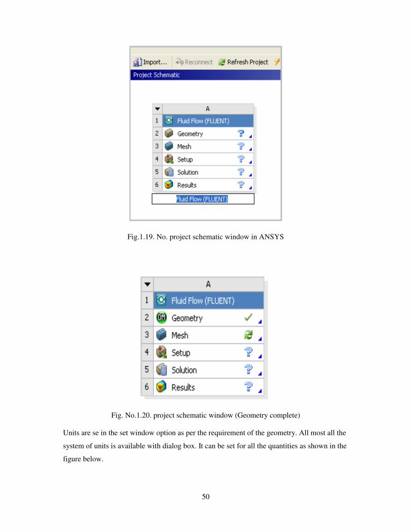
50
Fig.1.19. No. project schematic window in ANSYS
Fig. No.1.20. project schematic window (Geometry complete)
Units are se in the set window option as per the requirement of the geometry. All most all the
system of units is available with dialog box. It can be set for all the quantities as shown in the
figure below.

51
Fig. No.1.21. Set Unit Window Models Model can be defined as per the problem specification. The selection of model depends upon
the analysis. The fig below shows different models available for analysis purpose in the
ANSYS software.
Fig. No.1.22. Models in ANSYS

52
ANSYS also have the very rich material library with their specification and the slandered
value of properties. These properties can be read directly by software in case other special
characteristic have to define there is option of defining the property by edit option.
Fig. No.1.23. Create /Edit Materials
The boundary condition for problem analysis can be defined in the boundary condition dialog
box. The Fig.No.1.24 Shows the boundary condition dialog box in the ANSYS.

53
Fig. No.1.24. Boundary Condition dialog Box.
Fig. No. 1.25. Showing the File status

54
Fig.No.1.26. Dialog box for contours


![Media kit 2010[1].pdf low res..pdf-1](https://img.pdfslide.us/doc/110x75/58f19a9f1a28aba8488b45d9/media-kit-20101pdf-low-respdf-1.jpg)


![Case_Studies[1] (1).pdf](https://img.pdfslide.us/doc/110x75/55cf8fbc550346703b9f471e/casestudies1-1pdf.jpg)


![1 habit 1[1].pdf](https://img.pdfslide.us/doc/110x75/55cf92cb550346f57b999be7/1-habit-11pdf.jpg)