0802.3688

Lecture Notes on CMB Theory:

From Nucleosynthesis to Recombination

byWayne Hu

arX

iv:0

802.

3688

v1 [

astr

o-ph

] 2

5 Fe

b 20

08

Contents

CMB Theory from Nucleosynthesis to Recombination page 11 Introduction 12 Brief Thermal History 1

2.1 Nucleosynthesis and Prediction of the CMB 12.2 Thermalization and Spectral Distortions 42.3 Recombination 6

3 Temperature Anisotropy from Recombination 93.1 Anisotropy from Inhomogeneity 103.2 Acoustic Oscillation Basics 133.3 Gravito-Acoustic Oscillations 183.4 Baryonic Effects 223.5 Matter-Radiation Ratio 243.6 Damping 253.7 Information from the Peaks 27

4 Polarization Anisotropy from Recombination 324.1 Statistical Description 334.2 EB Harmonic Description 344.3 Thomson Scattering 354.4 Acoustic Polarization 364.5 Gravitational Waves 37

5 Discussion 37

ii

CMB Theory from Nucleosynthesis to Recombination

1 Introduction

These lecture notes comprise an introduction to the well-established physics and phenomenology ofthe cosmic microwave background (CMB) between big bang nucleosynthesis and recombination. Wetake our study through recombination since most of the temperature and polarization anisotropyobserved in the CMB formed during the recombination epoch when free electrons became bound intohydrogen and helium.

The other reason for considering only this restricted range from nucleosynthesis to recombinationis that these notes are meant to complement the other lectures of the XIX Canary Island WinterSchool of Astrophysics. While they are self-contained and complete in and of themselves, they omitimportant topics that will be covered elsewhere in this volume: namely inflation (Sabino Matarrese),observations (Bruce Partridge), statistical analysis (Licia Verde), secondary anisotropy (MatthiasBartelmann), and non-Gaussianity (Enrique Martinez-Gonzalez).

Furthermore the approach taken here of introducing only as much detail as necessary to buildphysical intuition is more suitable as a general overview rather than a rigorous treatment for trainingspecialists. As such these notes complement the more formal lecture notes for the Trieste schoolwhich may anachronistically be viewed as a continuation of these notes in the same notation (Hu2003).

The outline of these notes are as follows. We begin in §2 with a brief thermal history of the CMB.We discuss the temperature and polarization anisotropy and acoustic peaks from recombination in§3-4 and conclude in §5. We take units throughout with h = c = kB = 1 and illustrate effectsin the standard cosmological constant cold dark matter universe with adiabatic inflationary initialconditions (ΛCDM).

2 Brief Thermal History

In this section, we discuss the major events in the thermal history of the CMB. We begin in §2.1with the formation of the light elements and the original prediction of relic radiation. We continuein §2.2 with the processes that thermalize the CMB into a blackbody. Finally in §2.3, we discuss therecombination epoch where the main sources of temperature and polarization anisotropy lie.

2.1 Nucleosynthesis and Prediction of the CMB

Let us begin our brief thermal history with the relationship between the CMB and the abundanceof light elements established at an energy scale of 102 keV, time scale of a few minutes, temperature

1

2

3 minutes: nucleosynthesisfew months: thermalization

Fig. 1. A brief thermal history: nucleosynthesis, thermalization, recombination and reionization. Adaptedfrom Hu and White (2004).

of 109K and redshift of z ∼ 108 − 109. This is the epoch of nucleosynthesis, the formation of thelight elements. The qualitative features of nucleosynthesis are set by the low baryon-photon numberdensity of our universe. Historically, the sensitivity to this ratio was used by Gamow and collaboratorsin the late 1940’s to predict the existence and estimate the temperature of the CMB. Its modern useis the opposite: with the photon density well measured from the CMB spectrum, the abundance oflight elements determines the baryon density.

At the high temperature and densities of nucleosynthesis, radiation is rapidly thermalized to aperfect black body and the photon number density is a fixed function of the temperature nγ ∝ T 3

(see below). Apart from epochs in which energy from particle annihilation or other processes isdumped into the radiation, the baryon-photon number density ratio remains constant.

Likewise nuclear statistical equilibrium, while satisfied, makes the abundance of the light elementsof mass number A follow the expectations of a Maxwell-Boltzmann distribution for the phase spaceoccupation number

fA = e−(mA−µA)/T e−p2A/2mAT , (1)

where pA is the particle momentum, mA is the rest mass, and µA is the chemical potential. Namelytheir number density

nA ≡ gA

∫d3pA(2π)3

fA

= gA(mAT

2π)3/2e(µA−mA)/T . (2)

Here gA is the degeneracy factor. In equilibrium, the chemical potentials of the various elements arerelated to those of the proton and neutron by

µA = Zµp + (A− Z)µn , (3)

CMB Theory from Nucleosynthesis to Recombination 3

where Z is the charge or number of protons. Using this relation, the abundance fraction

XA ≡ AnAnb

= A5/2gA2−A[(

2πTmb

)3/2 2ζ(3)ηbγπ2

]A−1

eBA/TXZp X

A−Zn , (4)

where Xp and Xn are the proton and neutron abundance, ζ(3) ≈ 1.202, and nb is the baryon numberdensity. The two controlling quantities are the binding energy

BA = Zmp + (A− Z)mn −mA , (5)

and the baryon-photon number density ratio ηbγ = nb/nγ . That the latter number is of order 10−9

in our universe means that light elements form only well after the temperature has dropped belowthe binding energy of each species. Nuclear statistical equilibrium holds until the reaction rates dropbelow the expansion rate. At this point, the abundance freezes out and remains constant.

Gamow’s back of the envelope estimate (Gamow 1948, refined by Alpher and Herman 1948) wasto consider the neutron capture reaction that forms deuterium

n+ p↔ d+ γ (6)

with a binding energy of B2 = 2.2MeV. Given Eqn. (4)

X2 =3π2

(4πTmb

)3/2

ηbγζ(3)eB2/TXpXn , (7)

a low baryon-photon ratio, and Xn ≈ Xp ≈ 1/2 for estimation purposes, the critical temperaturefor deuterium formation is T ∼ 109K. In other words the low baryon-photon ratio means that thereare sufficient numbers of photons to dissociate deuterium until well below T ∼ B2. Note that thiscondition is only logarithmically sensitive to the exact value of the baryon-photon ratio chosen forthe estimate and so the reasoning is not circular.

Furthermore, that we observe deuterium at all and not all helium and heavier elements meansthat the reaction must have frozen out at near this temperature. Given the thermally averaged crosssection of

〈σv〉 ≈ 4.6× 10−20cm3s−1 , (8)

the freezeout condition

nb〈σv〉 ≈ H ≈ t−1 , (9)

and the time-temperature relation t(T = 109K) ≈ 180s from the radiation dominated Friedmannequation, we obtain an estimate of the baryon number density

nb(T = 109K) ∼ 1.2× 1017cm−3 . (10)

Comparing this density to the an observed current baryon density and requiring that nb ∝ a−3 andT ∝ a−1 yields the current temperature of the thermal background. For example, taking the modernvalue of Ωbh

2 ≈ 0.02 and nb(a = 1) = 2.2× 10−7cm−3 yields the rough estimate

T (a = 1) ≈ 12K . (11)

This value is of the same order of magnitude as the observed CMB temperature 2.725K as well asthe original estimates (Alpher and Herman 1948; Dicke et al. 1965). Modern day estimates of thebaryon-photon ratio also rely on deuterium (e.g. Tytler et al. 2000). We shall see that the CMB hasits own internal measure of this ratio from the acoustic peaks. Agreement between the nucleosynthesis

4

y-distortion

p/Tinit

0.1

0

-0.1

-0.2

10-3 10-2 10-1 1 101 102

Fig. 2. Comptonization process. Energy injected into the CMB through heating of the electrons is thermalizedby Compton scattering. Under the Kompaneets equation, a y-distortion first forms as low frequency photonsgain energy from the electrons. After multiple scatterings the distribution is thermalized to a chemical potentialor µ-distortion. Adapted from Hu (1995).

and acoustic peak measurements argue that the baryon-photon ratio has not changed appreciablysince z ∼ 108.

2.2 Thermalization and Spectral Distortions

Between nucleosynthesis and recombination, processes that create and destroy photons and hencethermalize the CMB fall out of equilibrium. The lack of spectral distortions in the CMB thusconstrains any process that injects energy or photons into the plasma after this epoch.

In a low baryon-photon ratio universe, the main thermalization process is double, also known asradiative, Compton scattering

e− + γ ↔ e− + γ + γ . (12)

The radiative Compton scattering rate becomes insufficient to maintain a blackbody at a redshift of(Danese and de Zotti 1982)

ztherm = 2.0× 106(1− Yp/2)−2/5

(Ωbh

2

0.02

)−2/5

(13)

corresponding to a time scale of order a few months.After this redshift, energy or photon injection appears as a spectral distortion in the spectrum of

the CMB. The form of the distortion is determined by Compton scattering

e− + γ ↔ e− + γ , (14)

since it is still sufficiently rapid compared with respect to the expansion while hydrogen remainsionized. Because a blackbody has a definite number density of photons at a given temperature,


ΔT

/Te

0

10-5 10-4 10-3 10-2 10-1 1 10

-0.05

-0.1

-0.15

p/Te

blackbody

z/105=3.5

0.5

z*

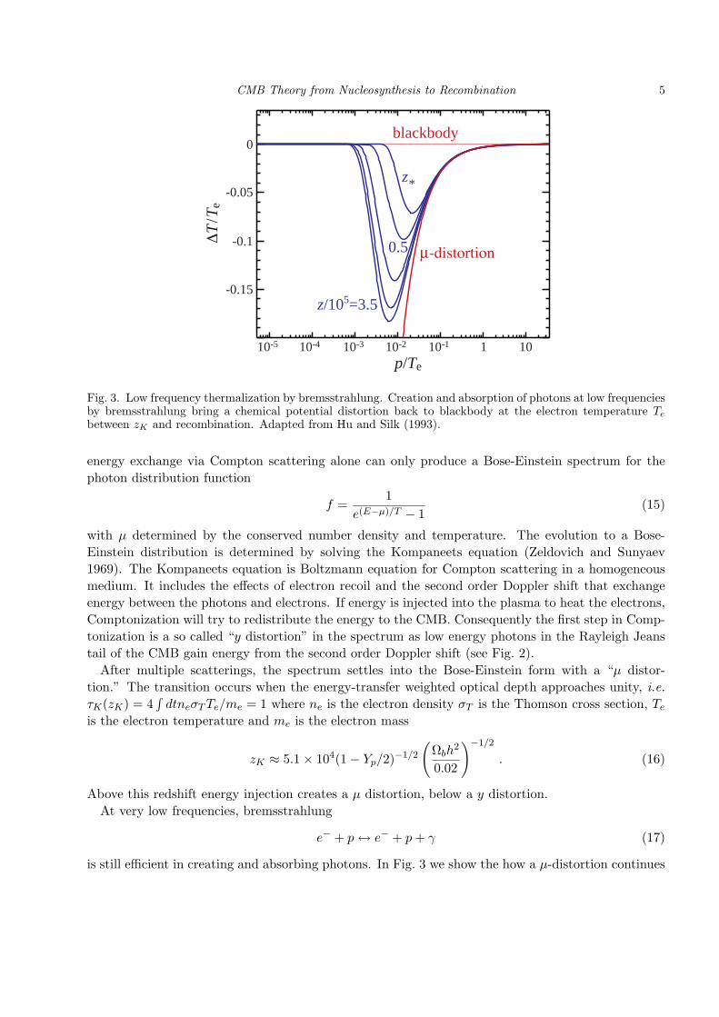
Fig. 3. Low frequency thermalization by bremsstrahlung. Creation and absorption of photons at low frequenciesby bremsstrahlung bring a chemical potential distortion back to blackbody at the electron temperature Tebetween zK and recombination. Adapted from Hu and Silk (1993).

energy exchange via Compton scattering alone can only produce a Bose-Einstein spectrum for thephoton distribution function

f =1

e(E−µ)/T − 1(15)

with µ determined by the conserved number density and temperature. The evolution to a Bose-Einstein distribution is determined by solving the Kompaneets equation (Zeldovich and Sunyaev1969). The Kompaneets equation is Boltzmann equation for Compton scattering in a homogeneousmedium. It includes the effects of electron recoil and the second order Doppler shift that exchangeenergy between the photons and electrons. If energy is injected into the plasma to heat the electrons,Comptonization will try to redistribute the energy to the CMB. Consequently the first step in Comp-tonization is a so called “y distortion” in the spectrum as low energy photons in the Rayleigh Jeanstail of the CMB gain energy from the second order Doppler shift (see Fig. 2).

After multiple scatterings, the spectrum settles into the Bose-Einstein form with a “µ distor-tion.” The transition occurs when the energy-transfer weighted optical depth approaches unity, i.e.τK(zK) = 4

∫dtneσTTe/me = 1 where ne is the electron density σT is the Thomson cross section, Te

is the electron temperature and me is the electron mass

zK ≈ 5.1× 104(1− Yp/2)−1/2

(Ωbh

2

0.02

)−1/2

. (16)

Above this redshift energy injection creates a µ distortion, below a y distortion.At very low frequencies, bremsstrahlung

e− + p↔ e− + p+ γ (17)

is still efficient in creating and absorbing photons. In Fig. 3 we show the how a µ-distortion continues

6

frequency (cm-1 )

GHz

error x50

5

0

2

4

6

8

10

12

10 15 20

200 400 600

Fig. 4. CMB spectrum from FIRAS. No spectral distortions from a blackbody have been discovered to date.

to evolve until recombination which brings the low frequency spectrum back to a blackbody but nowat the electron temperature.

The best limits to date are from COBE FIRAS from intermediate to high frequencies: |µ| < 9×10−5

and |y| < 1.5 × 10−5 at 95% confidence (see Fig 4 and Fixsen et al. 1996). After subtracting outgalactic emission, no spectral distortions of any kind are detected and the spectrum appears to be aperfect blackbody of T = 2.725± 0.002K (Mather et al. 1999).

2.3 Recombination

While the recombination process

p+ e− ↔ H + γ , (18)

is rapid compared to the expansion, the ionization fraction obeys an equilibrium distribution justlike that considered for light elements for nucleosynthesis or the CMB spectrum thermalization. Asin the former two processes, the qualitative behavior of recombination is determined by the lowbaryon-photon ratio of the universe.

Taking number densities of the Maxwell-Boltzmann form of Eqn. (2), we obtain

npnenH

≈ e−B/T(meT

2π

)3/2

e(µp+µe−µH)/T , (19)

where B = mp+me−mH = 13.6eV is the binding energy and we have set gp = ge = 12gH = 2. Given

the vanishingly small chemical potential of the photons, µp + µe = µH in equilibrium.Next, defining the ionization fraction for a hydrogen only plasma

np = ne = xenb ,

nH = nb − np = (1− xe)nb , (20)


Saha

2-levelx e io

niza

tion

frac

tion

scale factor a

redshift z

10-4

10-3

10-2

10-1

1

10-3

103104 102

10-2

Fig. 5. Hydrogen recombination in Saha equilibrium vs. the calibrated 2-level calculation of RECFAST. Thefeatures before hydrogen recombination are due to helium recombination.

we can rewrite Eqn. (19) as the Saha equation

nenpnHnb

=x2e

1− xe=

1nb

(meT

2π

)3/2

e−B/T . (21)

Recombination occurs at a temperature substantially lower than T = B again because of the lowbaryon-photon ratio of the universe. We can see this by rewriting the Saha equation in terms of thephoton number density

x2e

1− xe= e−B/kT

π1/2

25/2ηbγζ(3)

(mec

2

kT

)3/2

. (22)

Because ηbγ ∼ 10−9, the Saha equation implies that the medium only becomes substantially neutralat a temperature of T ≈ 0.3eV or at a redshift of z∗ ∼ 103. At this point, there are not enoughphotons in the even in the Wien tail above the binding energy to ionize hydrogen. We plot the Sahasolution in Fig. 5.

Near the epoch of recombination, the recombination rates become insufficient to maintain ionizationequilibrium. There is also a small contribution from helium recombination that must be added. Thecurrent standard for following the non-equilibrium ionization history is RECFAST (Seager et al. 2000)which employs the traditional two-level atom calculation of Peebles (1968) but alters the hydrogencase B recombination rate αB to fit the results of a multilevel atom. More specifically, RECFASTsolves a coupled system of equations for the ionization fraction xi in singly ionized hydrogen andhelium (i = H, He)

dxid ln a

=αBCinHp

H[s(xmax − xi)− xixe] , (23)

where nHp = (1− Yp)nb is the total hydrogen plus proton number density accounting for the helium

8

mass fraction Yp, xe ≡ ne/nHp =∑xi is the total ionization fraction, ne is the free electron density,

xmax is the maximum xi achieved through full ionization,

s =β

nHpe−B1s/Tb ,

C−1i = 1 +

βαBe−B2s/Tb

Λα + Λ2s1s,

β = grat

(Tbme

2π

)3/2

, (24)

with grat the ratio of statistical weights, Tb the baryon temperature, BL the binding energy of the Lthlevel, Λα the rate of redshifting out of the Lyman-α line corrected for the energy difference betweenthe 2s and 2p states

Λα =1π2

(B1s −B2p)3 e−(B2s−B2p)/Tb

H

(xmax − xi)nHp(25)

and Λ2s1s as the rate for the 2 photon 2s−1s transition. For reference, for hydrogen B1s = 13.598eV,B2s = B2p = B1s/4, Λ2s1s = 8.22458s−1, grat = 1, xmax = 1. For helium B1s = 24.583eV, B2s =3.967eV, B2p = 3.366eV, Λ2s1s = 51.3s−1, grat = 4, xmax = Yp/[4(1− Yp)].

Note that if the recombination rate is faster than the expansion rate αBCinHp/H 1, the ion-ization solutions for xi reach the Saha equilibrium dxi/d ln a = 0. In this case s(xmax − xi) = xixeor

xi =12

[√(xei + s)2 + 4sxmax − (xei + s)

](26)

= xmax

[1− xei + xmax

s

(1− xei + 2xmax

s

)+ ...

],

where xei = xe−xi is the ionization fraction excluding the species. The recombination of hydrogenicdoubly ionized helium is here handled purely through the Saha equation with a binding energy of1/4 the B1s of hydrogen and xmax = Yp/[4(1 − Yp)]. The case B recombination coefficients asa function of Tb are given in Seager et al. (2000) as is the strong thermal coupling between Tb andTCMB. The multilevel-atom fudge that RECFAST introduces is to replace the hydrogen αB → 1.14αBindependently of cosmology. While this fudge suffices for current observations, which approach the∼ 1% level, the recombination standard will require improvement if CMB anisotropy predictions areto reach an accuracy of 0.1% (e.g. Switzer and Hirata 2007; Wong et al. 2007).

The phenomenology of CMB temperature and polarization anisotropy is primarily governed by theredshift of recombination z∗ = a−1

∗ −1 when most of the contributions originate. This redshift thoughcarries little dependence on standard cosmological parameters. This insensitivity follows from thefact that recombination proceeds rapidly once B1s/Tb has reached a certain threshold as the Sahaequation illustrates. Defining the redshift of recombination as the epoch at which the Thomsonoptical depth during recombination (i.e. excluding reionization) reaches unity, τrec(a∗) = 1, a fit tothe recombination calculation gives (Hu 2005)

a−1∗ ≈ 1089

(Ωmh

2

0.14

)0.0105(Ωbh

2

0.024

)−0.028

, (27)

around a fiducial model of Ωmh2 = 0.14 and Ωbh

2 = 0.024.The universe is known to be reionized at low redshifts due to the lack of a Gunn-Peterson trough in


20

10 100 1000

40

60

80

100

[ l(

l+1)

Cl /

2π ]

1/2

(μK

)

64º

Fig. 6. From temperature maps to power spectrum. The original temperature fluctuation map (top left)corresponding to a simulation of the power spectrum (top right) can be band filtered to illustrate the powerspectrum in three characteristic regimes: the large-scale gravitational regime of COBE, the first acoustic peakwhere most of the power lies, and the damping tail where fluctuations are dissipated. Adapted from Hu andWhite (2004).

quasar absorption spectra. Moreover, large angle CMB polarization detections (see Fig. 19) suggestthat this transition back to full ionization occurred around z ∼ 10 leaving an extended neutral periodbetween recombination and reionization.

3 Temperature Anisotropy from Recombination

Spatial variations in the CMB temperature at recombination are seen as temperature anisotropy bythe observer today. The temperature anisotropy of the CMB was first detected in 1992 by the COBEDMR instrument (Smoot et al. 1992). These corresponded to variations of order ∆T/T ∼ 10−5 across10 − 90 on the sky (see Fig. 6).

Most of the structure in the temperature anisotropy however is associated with acoustic oscillationsof the photon-baryon plasma on ∼ 1 scales. Throughout the 1990’s constraints on the location of thefirst peak steadily improved culminating with the determinations of the TOCO (Miller et al. 1999),Boomerang, (de Bernardis et al. 2000) and Maxima-1 (Hanany et al. 2000) experiments. Currentlyfrom WMAP (Spergel et al. 2007) and ground based experiments, we have precise measurements ofthe first five acoustic peaks (see Fig. 7). Primary fluctuations beyond this scale (below ∼ 10′) aredamped by Silk damping (Silk 1968) as verified observationally first by the CBI experiment (Padinet al. 2001).

In this section, we deconstruct the basic physics behind these phenomena. We begin with thegeometric projection of temperature inhomogeneities at recombination onto the sky of the observerin §3.1. We continue with the basic equations of fluid mechanics that govern acoustic phenomena in§3.2. We add gravitational (§3.3), baryonic (§3.4), matter-radiation (§3.5), and dissipational (§3.6)

10

l(l+

1)C

l /2π

(μK

)2

l

Fig. 7. Temperature power spectrum from recent measurements from WMAP and ACBAR along with the bestfit ΛCDM model. The main features of the temperature power spectrum including the first 5 acoustic peaksand damping tail have now been measured. Adapted from Reichardt et al. (2008).

.

effects in the sections that follow. Finally we put these pieces back together to discuss the informationcontent of the acoustic peaks in §3.7.

3.1 Anisotropy from Inhomogeneity

Given that the CMB radiation is blackbody to experimental accuracy (see Fig. 4), one can characterizeits spatial and angular distribution by its temperature at the position x of the observer in the directionn on the observer’s sky

f(ν, n,x) = [exp(2πν/T (n; x)− 1]−1 , (28)

where ν = E/2π is the observation frequency. The hypothetical observer could be an electron in theintergalactic medium or the true observer on earth or L2. When the latter is implicitly meant, we willtake x = 0. We will occasionally suppress the coordinate x when this position is to be understood.

For statistically isotropic, Gaussian random temperature fluctuations a harmonic description ismore efficient than a real space description. For the angular structure at the position of the observer,the appropriate harmonics are the spherical harmonics. These are the eigenfunctions of the Laplaceoperator on the sphere and form a complete basis for scalar functions on the sky

Θ(n) =T (n)− T

T=∑`m

Θ`mY`m(n) . (29)

For statistically isotropic fluctuations, the ensemble average of the temperature fluctuations aredescribed by the power spectrum

〈Θ`m∗Θ`′m′〉 = δ``′δmm′C` . (30)

Moreover, the power spectrum contains all of the statistical information in the field if the fluctuationsare Gaussian. Here C` is dimensionless but is often shown with units of squared temperature, e.g.µK2, by multiplying through by the background temperature today T . The correspondence betweenangular size and amplitude of fluctuations and the power spectrum is shown in Fig. 6.

Let us begin with the simple approximation that the temperature field at recombination is isotropic


nD*

recombination

observer

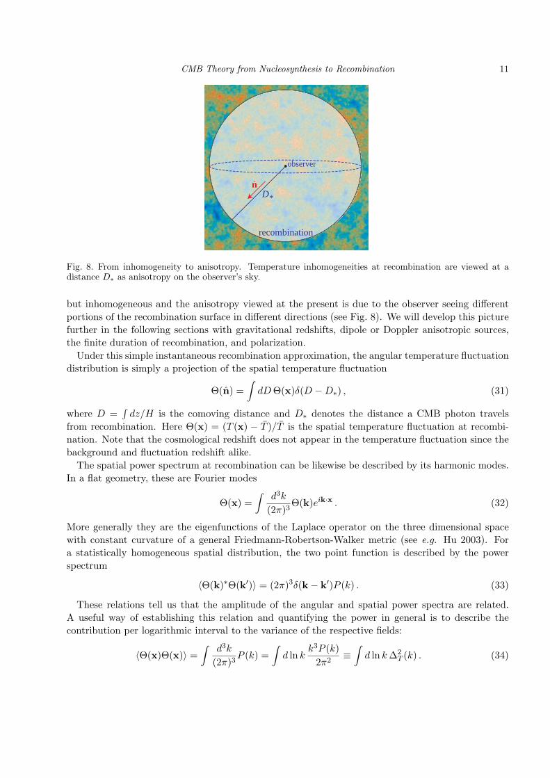
Fig. 8. From inhomogeneity to anisotropy. Temperature inhomogeneities at recombination are viewed at adistance D∗ as anisotropy on the observer’s sky.

but inhomogeneous and the anisotropy viewed at the present is due to the observer seeing differentportions of the recombination surface in different directions (see Fig. 8). We will develop this picturefurther in the following sections with gravitational redshifts, dipole or Doppler anisotropic sources,the finite duration of recombination, and polarization.

Under this simple instantaneous recombination approximation, the angular temperature fluctuationdistribution is simply a projection of the spatial temperature fluctuation

Θ(n) =∫dDΘ(x)δ(D −D∗) , (31)

where D =∫dz/H is the comoving distance and D∗ denotes the distance a CMB photon travels

from recombination. Here Θ(x) = (T (x) − T )/T is the spatial temperature fluctuation at recombi-nation. Note that the cosmological redshift does not appear in the temperature fluctuation since thebackground and fluctuation redshift alike.

The spatial power spectrum at recombination can be likewise be described by its harmonic modes.In a flat geometry, these are Fourier modes

Θ(x) =∫

d3k

(2π)3Θ(k)eik·x . (32)

More generally they are the eigenfunctions of the Laplace operator on the three dimensional spacewith constant curvature of a general Friedmann-Robertson-Walker metric (see e.g. Hu 2003). Fora statistically homogeneous spatial distribution, the two point function is described by the powerspectrum

〈Θ(k)∗Θ(k′)〉 = (2π)3δ(k− k′)P (k) . (33)

These relations tell us that the amplitude of the angular and spatial power spectra are related.A useful way of establishing this relation and quantifying the power in general is to describe thecontribution per logarithmic interval to the variance of the respective fields:

〈Θ(x)Θ(x)〉 =∫

d3k

(2π)3P (k) =

∫d ln k

k3P (k)2π2

≡∫d ln k∆2

T (k) . (34)

12

A scale invariant spectrum has equal contribution to the variance per e-fold ∆2T = k3P (k)/2π2 =

const. To relate this to the amplitude of the angular power spectrum, we expand equation (31) inFourier modes

Θ(n) =∫

d3k

(2π)3Θ(k)eik·D∗n . (35)

The Fourier modes themselves can be expanded in spherical harmonics with the relation

eikD∗·n = 4π∑`m

i`j`(kD∗)Y ∗`m(k)Y`m(n) , (36)

where j` is the spherical Bessel function. Extracting the multipole moments, we obtain

Θ`m =∫

d3k

(2π)3Θ(k)4πi`j`(kD∗)Y`m(k) . (37)

We can then relate the angular and spatial two point functions (30) and (33)

〈Θ∗`mΘ`′m′〉 = δ``′δmm′4π∫d ln k j2

` (kD∗)∆2T (k) = δ``′δmm′C` . (38)

Given a slowly varying, nearly scale invariant spatial power spectrum we can take ∆2T out of the

integral and evaluate it at the peak of the Bessel function kD∗ ≈ `. The remaining integral can beevaluated in closed form

∫∞0 j2

` (x)d lnx = 1/[2`(`+ 1)] yielding the final result

C` ≈2π

`(`+ 1)∆2T (`/D∗) . (39)

Likewise even slowly varying features like the acoustic peaks of §3.2 also mainly map to multipolesof ` ≈ kD∗ due to the delta function like behavior of j2

` .It is therefore common to plot the angular power spectrum as

C` ≡`(`+ 1)

2πC` ≈ ∆2

T . (40)

It is also common to plot C1/2` ≈ ∆T , the logarithmic contribution to the rms of the field, in units of

µK.Now let us compare this expression to the variance per log interval in multipole space:

〈T (n)T (n)〉 =∑`m

∑`′m′

〈T ∗`mT`′m′〉Y ∗`m(n)Y`′m′(n)

=∑`

C`∑m

Y ∗`m(n)Y`m(n) =∑`

2`+ 14π

C` . (41)

For variance contributions from ` 1,

∑`

2`+ 14π

C` ≈∫d ln `

`(2`+ 1)4π

C` ≈∫d ln `

`(`+ 1)2π

C` . (42)

Thus C` is also approximately the variance per log interval in angular space as well.


3.2 Acoustic Oscillation Basics

Thomson Tight Coupling — To understand the angular pattern of temperature fluctuations seen bythe observer today, we must understand the spatial temperature pattern at recombination. That inturn requires an understanding of the dominant physical processes in the plasma before recombination.

Thomson scattering of photons off of free electrons is the most important process given its relativelylarge cross section (averaged over polarization states)

σT =8πα2

3m2e

= 6.65× 10−25cm2 . (43)

The important quantity to consider is the mean free path of a photon given Thomson scatteringand a medium with a free electron density ne. Before recombination when the ionization fractionxe ≈ 1 this density is given by

ne = (1− Yp)xenb= 1.12× 10−5(1− Yp)xeΩbh

2(1 + z)3cm−3 . (44)

The comoving mean free path λC is given by

λ−1C ≡ τ ≡ neσTa , (45)

where the extra factor of a comes from converting physical to comoving coordinates and Yp is theprimordial helium mass fraction. We have also represented this mean free path in terms of anscattering absorption coefficient τ where dots are conformal time η ≡

∫dt/a derivatives and τ is the

optical depth.Near recombination (z ≈ 103, xe ≈ 1) and given Ωbh

2 ≈ 0.02, and Yp = 0.24, the mean free path is

λC ≡1τ∼ 2.5Mpc . (46)

This scale is almost two orders of magnitude smaller than the horizon at recombination. On scalesλ λC photons are tightly coupled to the electrons by Thomson scattering which in turn are tightlycoupled to the baryons by Coulomb interactions.

As a consequence, any bulk motion of the photons must be shared by the baryons. In fluidlanguage, the two species have a single bulk velocity vγ = vb and hence no entropy generation orheat conduction occurs. Furthermore, the shear viscosity of the fluid is negligible. Shear viscosity isrelated to anisotropy in the radiative pressure or stress and rapid scattering isotropizes the photondistribution. This is also the reason why in equation (31) we took the photon distribution to beisotropic but inhomogeneous.

We shall see that the fluid motion corrects this by allowing dipole ` = 1 anisotropy in the dis-tribution but no higher ` modes. It is only on scales smaller than the diffusion scale that radiativeviscosity (` = 2) and heat conduction becomes sufficiently large to dissipates the bulk motions of theplasma (see §3.6).

Zeroth Order Approximation — To understand the basic physical picture, let us begin our discussionof acoustic oscillations in the tight coupling regime with a simplified system which we will refine aswe progress.

First let us ignore the dynamical impact of the baryons on the fluid motion. Given that the baryonand photon velocity are equal and the momentum density of a relativistic fluid is given by (ρ+ p)v,

14

where p is the pressure, and v is the fluid velocity, this approximation relates to the quantity

R ≡ (ρb + pb)vb(ργ + pγ)vγ

=ρb + pbργ + pγ

=3ρb4ργ

≈ 0.6

(Ωbh

2

0.02

)(a

10−3

), (47)

where we have used the fact that ργ ∝ T 4 so that its value is fixed by the redshifting backgroundT = 2.725(1+z)K. Neglect of the baryon inertia and momentum only fails right around recombination.

Next, we shall assume that the background expansion is matter dominated to relate time and scalefactor. The validity of this approximation depends on the matter-radiation ratio

ρmρr

= 3.6

(Ωmh

2

0.15

)(a

10−3

), (48)

and is approximately valid during recombination and afterwords. One expects from these argumentsthat order unit differences between the real universe and our basic description will occur. We will infact use these differences in the following sections to show how the baryon and matter densities aremeasured from the acoustic peak morphology.

Finally, we shall consider the effect of pressure forces and neglect gravitational forces. While thisis not a valid approximation in and of itself, we shall see that for a photon-dominated system, theerror in ignoring gravitational forces exactly cancels with that from ignoring gravitational redshiftsthat photons experience after recombination (see §3.3).

Continuity Equation — Given that Thomson scattering neither creates nor destroys photons, thecontinuity equation implies that the photon number density only changes due to flows into and outof the volume. In a non expanding universe that would require

nγ +∇ · (nγvγ) = 0 . (49)

Since nγ is the number density of photons per unit physical (not comoving) volume, this equationmust be corrected for the expansion. The effect of the expansion can alternately be viewed as thatof the Hubble flow diluting the number density everywhere in space. Because number densities scaleas nγ ∝ a−3, the expansion alters the continuity equation as

nγ + 3nγa

a+∇ · (nγvγ) = 0 . (50)

Since we are interested in small fluctuations around the background, let us linearize the equationsnγ ≈ nγ + δnγ and drop terms that are higher than first order in δnγ/nγ and vγ . Note that vγ is firstorder in the number density fluctuations since as we shall see in the Euler equation discussion belowit is generated from the pressure gradients associated with density fluctuations.

The continuity equation (50) for the fluctuations becomes(δnγnγ

)·= −∇ · vγ . (51)

Since the number density nγ ∝ T 3, the fractional density fluctuation is related to the temperaturefluctuation Θ as

δnγnγ

= 3δT

T≡ 3Θ . (52)


Expressing the continuity equation in terms of Θ, we obtain

Θ = −13∇ · vγ . (53)

Fourier transforming this equation, we get

Θ = −13ik · vγ , (54)

for the relationship between the Fourier mode amplitudes.

Euler Equation — Now let us examine the origin of the fluid velocity. In the background, the velocityvanishes due to isotropy. However, Newtonian mechanics dictates that pressure forces will generateparticle momentum as q = F. Newton’s law must also be modified for the expansion. If weassociate the de Broglie wavelength with the inverse momentum, this wavelength also stretches withthe expansion. For photons, this accounts for the redshift factor. For non-relativistic matter, thismeans that bulk velocities decay with the expansion. In either case, we generalize Newton’s law toread

q +a

aq = F . (55)

For a collection of particles, the relevant quantity is the momentum density

(ργ + pγ)vγ ≡∫

d3q

(2π)3qf , (56)

and likewise the force becomes a force density. For the photon-baryon fluid, this force density isprovided by the pressure gradient. The result is the Euler equation

[(ργ + pγ)vγ ]· = −4a

a(ργ + pγ)vγ −∇pγ , (57)

where the 4 on the right hand side comes from combining the redshifting of wavelengths with that ofnumber densities. Since photons have an equation of state pγ = ργ/3, the Euler equation becomes

43ργvγ = −1

3∇ργ ,

vγ = −∇Θ . (58)

In Fourier space, the Euler equation becomes

vγ = −ikΘ . (59)

The factor of i here represents the fact that the temperature maxima and minima are zeros of thevelocity in real space due to the gradient relation, i.e. temperature and velocity have a π/2 phaseshift. It is convenient therefore to define the velocity amplitude to absorb this factor

vγ ≡ −ivγk . (60)

The direction of the fluid velocity is always parallel to the wavevector k for linear (scalar) perturba-tions and hence we can write the Euler equation as

vγ = kΘ . (61)

16

0

0.2 0.4 0.6 0.8s/s*

(a) Acoustic Oscillations

0.2 0.4 0.6 0.8s/s*

(b) Power Peaks

Fig. 9. Acoustic oscillation basics. All modes start from the same initial epoch with time denoted by thesound horizon relative to the sound horizon at recombination s∗. (a) Wavenumbers that reach extrema intheir effective temperature Θ + Ψ (accounting for gravitational redshifts §3.3) at s∗ form a harmonic serieskn = nπ/s∗. (b) Amplitude of the fluctuations is the same for the maxima and minima without baryon inertia.Adapted from Hu and Dodelson (2002).

Acoustic Peaks — Combining the continuity (54) and Euler (61) equations to eliminate the fluidvelocity, we get the simple harmonic oscillator equation

Θ + c2sk

2Θ = 0 , (62)

where the adiabatic sound speed c2s = 1/3 for the photon-dominated fluid and more generally is

defined as

c2s ≡

pγργ. (63)

The solution to the oscillator equation can be specified given two initial conditions Θ(0) and vγ(0)or Θ(0),

Θ(η) = Θ(0) cos(ks) +Θ(0)kcs

sin(ks) , (64)

where the sound horizon is defined as

s ≡∫csdη . (65)

In real space, these oscillations appear as standing waves for each Fourier mode.These standing waves continue to oscillate until recombination. At this point the free electron

density drops drastically (see Fig. 5) and the photons freely stream to the observer. The pattern ofacoustic oscillations on the recombination surface seen by the observer becomes the acoustic peaksin the temperature anisotropy.

Let us focus on the adiabatic mode which starts with a finite density or temperature fluctuationand vanishing velocity perturbation. At recombination η∗, the oscillation reaches (see Fig. 9)

Θ(η∗) = Θ(0) cos(ks∗) . (66)

Considering a spectrum of k modes, the critical feature of these oscillations are that they are tempo-rally coherent. The underlying assumption is that fluctuations of all wavelengths originated at η = 0or at least η η∗. Without inflation this would violate causality for long wavelength fluctuations, i.e.


the analogue of the horizon problem for perturbations. With inflation, superhorizon modes originateduring an inflationary epoch ηi η∗.

Modes caught in the extrema of their oscillation follow a harmonic relation

kns∗ = nπ , n = 1, 2, 3 . . . (67)

yielding a fundamental scale or frequency, related to the inverse sound horizon

kA = π/s∗ . (68)

Since the power spectrum is proportional to the square of the fluctuation, both maxima and minimacontribute peaks in the spectrum. Observational verification of this harmonic series is the primaryevidence for inflationary adiabatic initial conditions (Hu and White 1996).

The fundamental physical scale is translated into a fundamental angular scale by simple projectionaccording to the angular diameter distance DA

θA = λA/DA ,

À = kADA , (69)

(see Eqn. (39)). In a flat universe, the distance is simply DA = D ≡ η0 − η∗ ≈ η0, the horizondistance, and kA = π/s∗ =

√3π/η∗ so

θA ≈η∗η0. (70)

Furthermore, in a matter-dominated universe η ∝ a1/2 so θA ≈ 1/30 ≈ 2 or

À ≈ 200 . (71)

We shall see in §3.7 that radiation and dark energy introduce important corrections to this predictionfrom their influence on η∗ and D∗ respectively. Nonetheless it is remarkable that this simple argumentpredicts the basics of acoustic oscillations: their existence, coherence and fundamental scale.

Acoustic Troughs: Doppler Effect — Acoustic oscillations also imply that the plasma is movingrelative to the observer. This bulk motion imprints a temperature anisotropy via the Doppler effect(

∆TT

)dop

= n · vγ . (72)

Averaged over directions (∆TT

)rms

=vγ√

3, (73)

which given the acoustic solution of Eqn. (64) implies

vγ√3

= −√

3k

Θ =√

3kkcs Θ(0)sin(ks)

= Θ(0)sin(ks) . (74)

Interestingly, the Doppler effect for the photon-dominated system is of equal amplitude and π/2out of phase: extrema of temperature are turning points of velocity. If we simply add the k-spacetemperature and Doppler effects in quadrature we would obtain(

∆TT

)2

= Θ2(0)[cos2(ks) + sin2(ks)] = Θ2(0) . (75)

18

5

10

5

500 1000 1500 2000

10

Ang

ular

Pow

erSp

atia

l Pow

er

l

kD*

Total

TemperatureDoppler

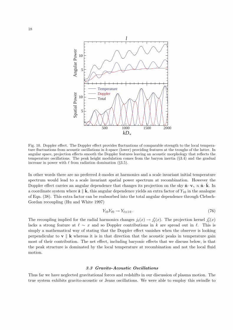
Fig. 10. Doppler effect. The Doppler effect provides fluctuations of comparable strength to the local tempera-ture fluctuations from acoustic oscillations in k-space (lower) providing features at the troughs of the latter. Inangular space, projection effects smooth the Doppler features leaving an acoustic morphology that reflects thetemperature oscillations. The peak height modulation comes from the baryon inertia (§3.4) and the gradualincrease in power with ` from radiation domination (§3.5).

In other words there are no preferred k-modes at harmonics and a scale invariant initial temperaturespectrum would lead to a scale invariant spatial power spectrum at recombination. However theDoppler effect carries an angular dependence that changes its projection on the sky n ·vγ ∝ n · k. Ina coordinate system where z ‖ k, this angular dependence yields an extra factor of Y10 in the analogueof Eqn. (38). This extra factor can be reabsorbed into the total angular dependence through Clebsch-Gordan recoupling (Hu and White 1997)

Y10Y`0 → Y`±1 0 . (76)

The recoupling implied for the radial harmonics changes j`(x) → j′`(x). The projection kernel j′`(x)lacks a strong feature at ` ∼ x and so Doppler contributions in k are spread out in `. This issimply a mathematical way of stating that the Doppler effect vanishes when the observer is lookingperpendicular to v ‖ k whereas it is in that direction that the acoustic peaks in temperature gainmost of their contribution. The net effect, including baryonic effects that we discuss below, is thatthe peak structure is dominated by the local temperature at recombination and not the local fluidmotion.

3.3 Gravito-Acoustic Oscillations

Thus far we have neglected gravitational forces and redshifts in our discussion of plasma motion. Thetrue system exhibits gravito-acoustic or Jeans oscillations. We were able to employ this swindle to


get the basic properties of acoustic oscillations because in a photon-dominated plasma the effect ofgravitational forces and gravitational redshifts exactly cancel in constant gravitational potentials. Togo beyond the photon dominated plasma and matter dominated expansion approximation, we nowneed to include these effects. Furthermore, we shall see that the gravitational potential perturbationsfrom inflation are also the source of the initial temperature fluctuation.

Continuity Equation and Newtonian Curvature — The photon continuity equation for the numberdensity is altered by gravity since the presence of a gravitational potential alters the coordinatevolume. Formally in general relativity this comes from the space-space piece of the metric – a spatialcurvature perturbation Φ:

ds2 = a2[−(1 + 2Ψ)dη2 + (1 + 2Φ)dx2] (77)

for a flat cosmology.We can think of this curvature perturbation as changing the local scale factor a→ a(1 + Φ) so that

the expansion dilution is generalized to

a

a→ a

a+ Φ . (78)

Hence the full continuity equation is now given by

(δnγ)· = −3δnγa

a− 3nγΦ− nγ∇ · vγ , (79)

or

Θ = −13kvγ − Φ . (80)

Euler Equation and Newtonian Forces — Likewise the gravitational force from gradients in the gravi-tational potential (Ψ, formally the time-time piece of the metric perturbation) modifies the momentumconservation equation. The Newtonian force F = −m∇Ψ generalized to momentum density bringsthe Euler equation to

vγ = k(Θ + Ψ) . (81)

General relativity says that Φ and Ψ are the relativistic analogues of the Newtonian potential andthat Φ ≈ −Ψ in the absence of sources of anisotropic stress or viscosity.

Photon Dominated Oscillator — We can again combine the continuity equation (80) and Euler equa-tion (81) to form the forced simple harmonic oscillator system

Θ + c2sk

2Θ = −k2

3Ψ− Φ . (82)

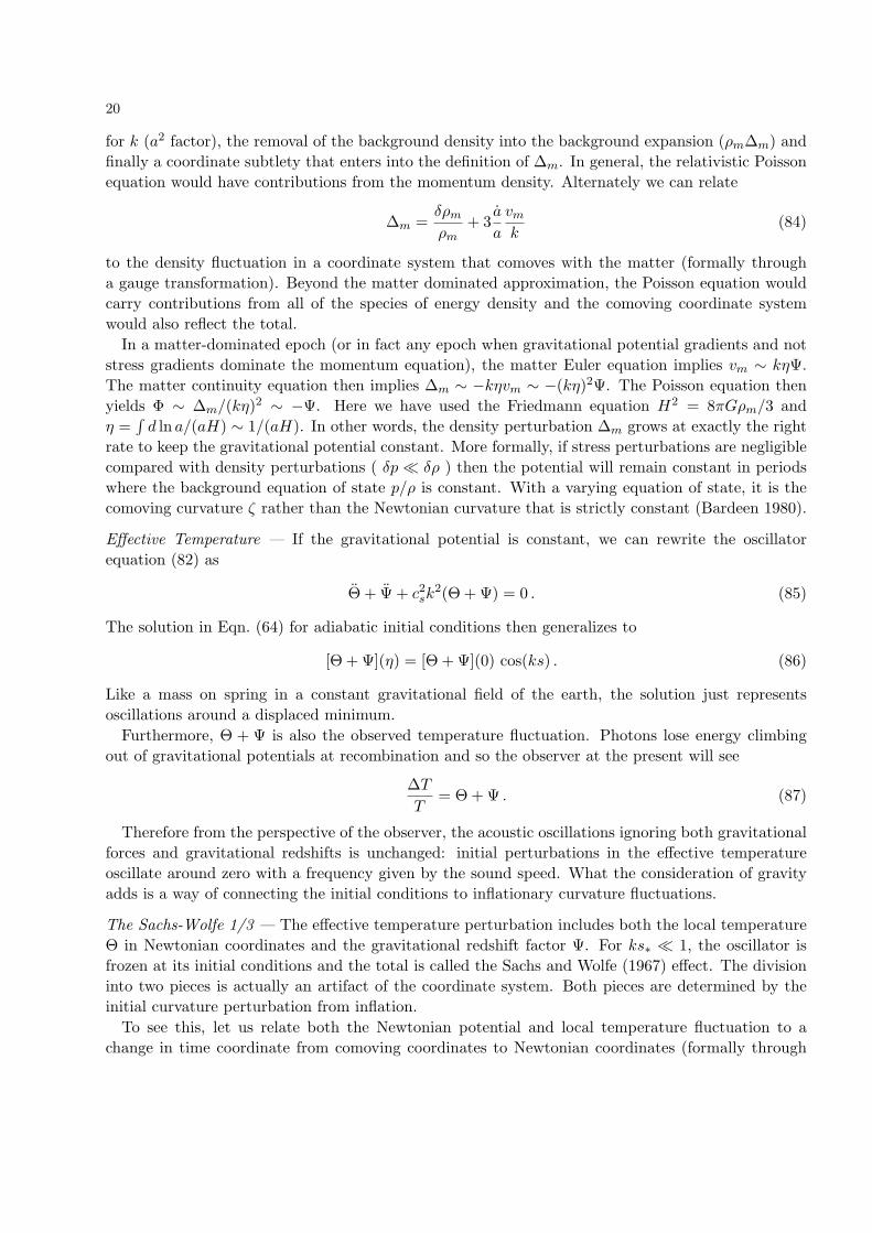
Note that the effect of baryon inertia is still absent in this system. To make further progress in un-derstanding the effect of gravity on acoustic oscillations we need to specify the gravitational potentialΨ ≈ −Φ from the Poisson equation and understand its time evolution.

Poisson Equation and Constant Potentials — In our matter-dominated approximation, Φ is generatedby matter density fluctuations ∆m through the cosmological Poisson equation

k2Φ = 4πGa2ρm∆m , (83)

where the difference from the usual Poisson equation comes from the use of comoving coordinates

20

for k (a2 factor), the removal of the background density into the background expansion (ρm∆m) andfinally a coordinate subtlety that enters into the definition of ∆m. In general, the relativistic Poissonequation would have contributions from the momentum density. Alternately we can relate

∆m =δρmρm

+ 3a

a

vmk

(84)

to the density fluctuation in a coordinate system that comoves with the matter (formally througha gauge transformation). Beyond the matter dominated approximation, the Poisson equation wouldcarry contributions from all of the species of energy density and the comoving coordinate systemwould also reflect the total.

In a matter-dominated epoch (or in fact any epoch when gravitational potential gradients and notstress gradients dominate the momentum equation), the matter Euler equation implies vm ∼ kηΨ.The matter continuity equation then implies ∆m ∼ −kηvm ∼ −(kη)2Ψ. The Poisson equation thenyields Φ ∼ ∆m/(kη)2 ∼ −Ψ. Here we have used the Friedmann equation H2 = 8πGρm/3 andη =

∫d ln a/(aH) ∼ 1/(aH). In other words, the density perturbation ∆m grows at exactly the right

rate to keep the gravitational potential constant. More formally, if stress perturbations are negligiblecompared with density perturbations ( δp δρ ) then the potential will remain constant in periodswhere the background equation of state p/ρ is constant. With a varying equation of state, it is thecomoving curvature ζ rather than the Newtonian curvature that is strictly constant (Bardeen 1980).

Effective Temperature — If the gravitational potential is constant, we can rewrite the oscillatorequation (82) as

Θ + Ψ + c2sk

2(Θ + Ψ) = 0 . (85)

The solution in Eqn. (64) for adiabatic initial conditions then generalizes to

[Θ + Ψ](η) = [Θ + Ψ](0) cos(ks) . (86)

Like a mass on spring in a constant gravitational field of the earth, the solution just representsoscillations around a displaced minimum.

Furthermore, Θ + Ψ is also the observed temperature fluctuation. Photons lose energy climbingout of gravitational potentials at recombination and so the observer at the present will see

∆TT

= Θ + Ψ . (87)

Therefore from the perspective of the observer, the acoustic oscillations ignoring both gravitationalforces and gravitational redshifts is unchanged: initial perturbations in the effective temperatureoscillate around zero with a frequency given by the sound speed. What the consideration of gravityadds is a way of connecting the initial conditions to inflationary curvature fluctuations.

The Sachs-Wolfe 1/3 — The effective temperature perturbation includes both the local temperatureΘ in Newtonian coordinates and the gravitational redshift factor Ψ. For ks∗ 1, the oscillator isfrozen at its initial conditions and the total is called the Sachs and Wolfe (1967) effect. The divisioninto two pieces is actually an artifact of the coordinate system. Both pieces are determined by theinitial curvature perturbation from inflation.

To see this, let us relate both the Newtonian potential and local temperature fluctuation to achange in time coordinate from comoving coordinates to Newtonian coordinates (formally through


105 15 20

damping

driving

Fig. 11. Acoustic oscillations with gravitational forcing and dissipational damping. For a mode that entersthe sound horizon during radiation domination, the gravitational potential decays at horizon crossing anddrives the acoustic amplitude higher. As the photon diffusion length increases and becomes comparable tothe wavelength, radiative viscosity πγ is generated from quadrupole anisotropy leading to dissipation andpolarization (see §4.4). Adapted from Hu and Dodelson (2002).

a gauge transformation, see White and Hu 1997 for a more detailed treatment). The Newtoniangravitational potential Ψ is a perturbation to the temporal coordinate (see Eqn. (77))

δt

t= Ψ . (88)

Given the Friedmann equation, this is equivalent to a perturbation in the scale factor

t =∫

da

aH∝∫

da

aρ1/2∝ a3(1+w)/2 , (89)

where w ≡ p/ρ. During matter domination w = 0 and

δa

a=

23δt

t. (90)

Since the CMB temperature is cooling as T ∝ a−1 a local change in the scale factor changes thelocal temperature

Θ = −δaa

= −23

Ψ . (91)

Combining this with Ψ to form the effective temperature gives

Θ + Ψ =13

Ψ . (92)

The consequence is that overdense regions where Ψ is negative (potential wells) are cold spots in theeffective temperature.

Inflation provides a source for initial curvature fluctuations. Specifically the comoving curvatureperturbation ζ becomes a Newtonian curvature of

Φ =35ζ (93)

22

0.2 0.4 0.6 0.8s/s*

R=1/6

Baryons

0

Fig. 12. Acoustic oscillations with baryons. Baryons add inertia to the photon-baryon plasma displacing thezero point of the oscillation and making compressional peaks (minima) larger than rarefaction peaks (maxima).The absolute value of the fluctuation in effective temperature is shown in dotted lines. Adapted from Hu andDodelson (2002).

in the matter-dominated epoch. The initial amplitude of scalar curvature perturbations is usuallygiven as AS = δ2

ζ which characterizes the variance contribution per e-fold to the curvature near somefiducial wavenumber kn (see Eqn. 34)

∆2ζ =

k3Pζ2π2

= δ2ζ

(k

kn

)n−1

, (94)

where n = 1 for a scale invariant spectrum. Combining these relations for n = 1

`(`+ 1)C`2π

≈δ2ζ

25. (95)

in the Sachs-Wolfe limit. The 10−5 fluctuations measured by COBE then correspond to δζ ≈ 5×10−5.

3.4 Baryonic Effects

The next level of detail that we need to add is the inertial effect of baryons in the plasma. Sinceequation (47) says that the baryon momentum becomes comparable to the photon momentum nearrecombination, we can expect order unity corrections on the basic acoustic oscillation picture frombaryons. With the precise measurements of the first and second peak, this change in the acousticmorphology has already provided the most sensitive measure of the baryon-photon ratio to dateexceeding that of big bang nucleosynthesis.

Baryon Loading — Baryons add extra mass to the photon-baryon plasma or equivalently an enhance-ment of the momentum density of the plasma given by R = (pb + ρb)/(pγ + ργ). Specifically themomentum density of the joint system

(ργ + pγ)vγ + (ρb + pb)vb ≡ (1 +R)(ργ + pγ)vγb (96)

is conserved. For generality, we have introduced the baryon velocity vb and the momentum-weightedvelocity vγb but in the tightly coupled plasma vb ≈ vγb ≈ vγ (c.f. §3.6).


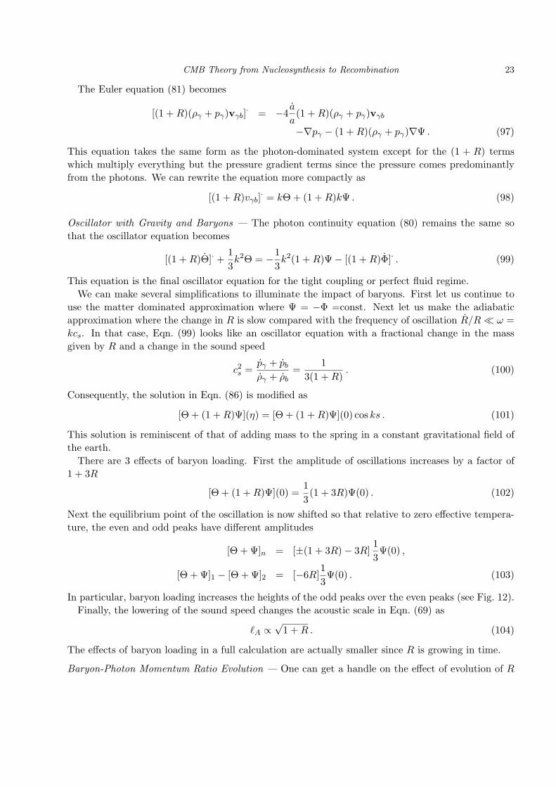
The Euler equation (81) becomes

[(1 +R)(ργ + pγ)vγb]· = −4a

a(1 +R)(ργ + pγ)vγb

−∇pγ − (1 +R)(ργ + pγ)∇Ψ . (97)

This equation takes the same form as the photon-dominated system except for the (1 + R) termswhich multiply everything but the pressure gradient terms since the pressure comes predominantlyfrom the photons. We can rewrite the equation more compactly as

[(1 +R)vγb]· = kΘ + (1 +R)kΨ . (98)

Oscillator with Gravity and Baryons — The photon continuity equation (80) remains the same sothat the oscillator equation becomes

[(1 +R)Θ]· +13k2Θ = −1

3k2(1 +R)Ψ− [(1 +R)Φ]· . (99)

This equation is the final oscillator equation for the tight coupling or perfect fluid regime.We can make several simplifications to illuminate the impact of baryons. First let us continue to

use the matter dominated approximation where Ψ = −Φ =const. Next let us make the adiabaticapproximation where the change in R is slow compared with the frequency of oscillation R/R ω =kcs. In that case, Eqn. (99) looks like an oscillator equation with a fractional change in the massgiven by R and a change in the sound speed

c2s =

pγ + pbργ + ρb

=1

3(1 +R). (100)

Consequently, the solution in Eqn. (86) is modified as

[Θ + (1 +R)Ψ](η) = [Θ + (1 +R)Ψ](0) cos ks . (101)

This solution is reminiscent of that of adding mass to the spring in a constant gravitational field ofthe earth.

There are 3 effects of baryon loading. First the amplitude of oscillations increases by a factor of1 + 3R

[Θ + (1 +R)Ψ](0) =13

(1 + 3R)Ψ(0) . (102)

Next the equilibrium point of the oscillation is now shifted so that relative to zero effective tempera-ture, the even and odd peaks have different amplitudes

[Θ + Ψ]n = [±(1 + 3R)− 3R]13

Ψ(0) ,

[Θ + Ψ]1 − [Θ + Ψ]2 = [−6R]13

Ψ(0) . (103)

In particular, baryon loading increases the heights of the odd peaks over the even peaks (see Fig. 12).Finally, the lowering of the sound speed changes the acoustic scale in Eqn. (69) as

À ∝√

1 +R . (104)

The effects of baryon loading in a full calculation are actually smaller since R is growing in time.

Baryon-Photon Momentum Ratio Evolution — One can get a handle on the effect of evolution of R

24

by again equating the system to the analogous physical oscillator. The baryons add inertia or massto the system and for a slowly varying mass the oscillator equation has an adiabatic invariant

E

ω=

12meffωA

2 =12

(1 +R)kcsA2 ∝ A2(1 +R)1/2 = const. (105)

Amplitude of oscillation A ∝ (1 + R)−1/4 decays adiabatically as the photon-baryon ratio changes.This offsets the gain in the overall amplitude from Eqn. (102). Coupled with uncertainties in thedistance to recombination in interpreting the À measurement, this leaves the modulation of the peakheights as the effect that provides most of the information about the baryon-photon ratio in theacoustic peaks.

3.5 Matter-Radiation Ratio

Next we want to go beyond the matter-dominated expansion approximation. The universe only be-comes matter dominated in the few e-folds before recombination (see Eqn. (48)). Peaks correspondingto wavenumbers that began oscillating earlier carry the effects of the prior epoch of radiation dom-ination. These effects come in through the evolution of the gravitational potential which acts as aforcing function on the oscillator through Eqn. (99).

Potential Decay — The argument given in §3.3 for the constancy of the gravitational potential dependscrucially on gravity being the dominant force affecting the total density. When radiation dominatesthe total density, radiation stresses become more important than gravity on scales smaller than thesound horizon. The total density fluctuation stops growing and instead oscillates with the acousticfrequency. The Poisson equation in the radiation dominated epoch

k2Φ = 4πGa2ρr∆r (106)

then implies that Φ oscillates and decays with an amplitude ∝ a−2 (see Fig. 11). As an aside, therelativistic stresses of dark energy make the gravitational potential decay again during the accelerationepoch and lead to the so called integrated Sachs-Wolfe effect.

Radiation Driving — An examination of Fig. 11 shows that the time evolution of the gravitationalpotential is in phase with the acoustic oscillations themselves and act a driving force on the acousticoscillations. We can estimate the effect on the amplitude of oscillations in the limit that the force isfully coherent. In that case we can take the continuity equation (80) and simply integrate it

[Θ + Ψ](η) = [Θ + Ψ](0) + ∆Ψ−∆Φ

= 13Ψ(0)− 2Ψ(0) = 5

3Ψ(0) . (107)

This estimate gives an acoustic amplitude that is 5× that of the Sachs-Wolfe effect. This enhancementonly occurs for modes that begin oscillating during the radiation dominated epoch, i.e. the higherpeaks. The net effect is a gradual ramp up of the acoustic oscillation amplitude across the horizonwavenumber at matter radiation equality (see Fig. 10).

In fact the coherent approximation is exact for a photon-baryon fluid but must be corrected forthe neutrino contribution to the radiation density.

External Potential Approach — For pedagogical purposes it is sometimes useful to go beyond thecoherent approximation. Neutrino corrections are one example; isocurvature initial conditions areanother.


We have seen that the solutions to homogeneous equation for the oscillator equation (82) are

(1 +R)−1/4cos(ks) , (1 +R)−1/4sin(ks) (108)

in the adiabatic or high frequency limit. Considering the potentials as external, we can solve for thetemperature perturbation as (Hu and Sugiyama 1995)

(1 +R)1/4Θ(η) = Θ(0)cos(ks) +√

3k

[Θ(0) + 1

4R(0)Θ(0)]

sin ks

+√

3k

∫ η0 dη

′(1 +R′)3/4sin[ks− ks′]F (η′) , (109)

where

F = −Φ− R

1 +RΦ− k2

3Ψ . (110)

By including the neutrino effects in the gravitational potential, we can show from this approach thatradiation driving actually creates an acoustic amplitude that is close to 4× the Sachs-Wolfe effect.

3.6 Damping

The final piece in the acoustic oscillation puzzle is the damping of power beyond ` ∼ 103 shown inFig. 6. Up until this point, we have considered the oscillations in the tight coupling approximationwhere the photons and baryons respond to pressure and gravity as a single perfect fluid. Fluidimperfections are associated with the Compton mean free path in Eqn. (46). Dissipation becomesstrong at the diffusion scale, the distance a photon can random walk in a given time η (Silk 1968)

λD =√NλC =

√η/λC λC =

√ηλC . (111)

This scale is the geometric mean between the horizon and mean free path. Given that λD/η∗ ∼ fewpercent, we expect that the n ≥ 3 peaks to be affected by dissipation. To improve on this estimate,we develop the microphysical description of dissipation next.

Continuity Equations — To treat the photons and baryons as separate systems, we now need tosupplement the photon continuity equation with the baryon continuity equation

Θ = −k3vγ − Φ , δb = −kvb − 3Φ . (112)

The baryon equation follows from number conservation with ρb = mbnb and δb ≡ δρb/ρb.

Euler and Navier-Stokes Equations — The momentum conservation equations must also be separatedinto photon and baryon pieces

vγ = k(Θ + Ψ)− k

6πγ − τ(vγ − vb) ,

vb = − aavb + kΨ + τ(vγ − vb)/R ,

where the photons gain an anisotropic stress term πγ from radiation viscosity. The baryon equationfollows from the same derivation as in §3.2 where the redshift of the momentum is carried by thebulk velocity instead of the redshifting temperature. Finally there is a momentum exchange termfrom Compton scattering. Note that the total momentum in the system is conserved and hence thescattering terms come with opposite sign.

26

Viscosity — Radiative shear viscosity is equivalent to quadrupole moments in the temperature field.These quadrupole moments are generated by radiation streaming from hot to cold regions much likehow temperature inhomogeneity are converted to anisotropy in Fig. 8.

In the tight coupling limit where τ /k, the optical depth through a wavelength of the fluctuation ishigh one therefore expects

πγ ∼ vγk

τ, (113)

since it must be generated by streaming and suppressed by scattering. A more detailed calculationfrom the Boltzmann or radiative transfer equation says (Kaiser 1983)

πγ ≈ 2Avvγk

τ, (114)

where Av = 16/15 once polarization effects are incorporated

vγ = k(Θ + Ψ)− k

3Av

k

τvγ . (115)

The oscillator equation with viscosity becomes

c2s

d

dη(c−2s Θ) +

k2c2s

τAvΘ + k2c2

sΘ = −k2

3Ψ− c2

s

d

dη(c−2s Φ) ,

As in a mechanical oscillator, a term that depends on Θ provides a dissipational term to the solutions.

Heat Conduction — Relative motion between the photons and baryons also damp oscillations. Byexpanding the continuity and momentum conservation equations in the small number k/τ one obtainsfor the full oscillator equation

c2s

d

dη(c−2s Θ) +

k2c2s

τ[Av +Ah]Θ + k2c2

sΘ = −k2

3Ψ− c2

s

d

dη(c−2s Φ)

where

Ah =R2

1 +R. (116)

Dispersion Relation — We can solve the damped oscillator equation in the adiabatic approximationby taking a trial solution Θ ∝ exp(i

∫ωdη) to obtain the dispersion relation

ω = ±kcs[1± i

2kcsτ

(Av +Ah)]. (117)

The imaginary term in the dispersion relation gives an exponential damping of the oscillation ampli-tude

exp(i∫ωdη) = e±iks exp[−k2

∫dη

12c2s

τ(Av +Ah)]

= e±iks exp[−(k/kD)2] , (118)

where the diffusion wavenumber is given by

k−2D =

∫dη

1τ

16(1 +R)

(1615

+R2

(1 +R)

). (119)


Note that in both the high and low R limits

limR→0

k−2D =

16

1615

∫dη

1τ,

limR→∞

k−2D =

16

∫dη

1τ. (120)

Hence the dissipation scale is

λD =2πkD∼ 2π√

6(ητ−1)1/2 (121)

and comparable to the geometric mean between horizon and mean free path as expected from therandom walk argument . For a baryon density of Ωbh

2 ≈ 0.02, radiation viscosity is responsible formost of the dissipation and we show the correspondence between viscosity generation and dissipationin Fig. 11.

Since the diffusion length changes rapidly through recombination and the medium changes fromoptically thick to optically thin, the damping estimates above are only qualitative. A full Boltzmann(radiative transfer solution) shows a more gradual, but still exponential, damping of roughly

D` ≈ exp[−(`/`D)1.25] , (122)

with a damping scale of `D = 2πD∗/λD and (Hu 2005)

λDMpc

≈ 64.5

(Ωmh

2

0.14

)−0.278(Ωbh

2

0.024

)−0.18

, (123)

for small changes around the central values of Ωmh2 and Ωbh

2.This envelope also accounts for enhanced damping due to the finite duration of recombination.

Instead of a delta function in the projection equation (31) we have the visibility function τ e−τ thatacts as a smearing out of any contributions with wavelengths shorter than the thickness of therecombination surface that survive dissipation.

3.7 Information from the Peaks

In the preceding sections we have examined the physical processes involved in the formation of theacoustic peaks and explained their sensitivity to the energy content and expansion rate of the universe.Converting the measurements into parameter constraints of course requires a more accurate numericaldescription. Numerical codes that solve the Einstein-Boltzmann radiative transfer equations for theCMB and matter (Peebles and Yu 1970; Bond and Efstathiou 1984; Vittorio and Silk 1984) are nowaccurate at the ∼ 1% level for the acoustic peaks for publically available codes (Seljak and Zaldarriaga1996; Lewis et al. 2000). Their numerical precision on the other hand is substantially better andapproaches the 0.1% level required for cosmic variance limited measurements out to ` ∼ 103. Theaccuracy is now limited by the input physics, mainly recombination (see 2.3). In this section, werelate the qualitative discussion of the previous sections to the quantitative information content ofthe peaks.

First Peak: Curvature and Dark Energy — The comparison between the predicted acoustic peak scaleλA and its angular extent provides a measurement of the angular diameter distance to recombination.The angular diameter distance in turn depends on the spatial curvature and expansion history of theuniverse.

28

D

LDA

Fig. 13. Angular diameter distance and curvature. In a non-flat (here closed) universe, the apparent or angulardiameter distance DA = Ldα does not equal the radial distance traveled by the photon. Objects in a closeduniverse are further than they appear whereas in an open universe they are closer than they appear.

Sensitivity to the expansion history during the acceleration epoch comes about through the radialdistance a photon travels along the line of sight

D∗ =∫ z∗

0

dz

H(z)= η0 − η∗ . (124)

With the matter and radiation energy densities measured, the remaining contributor to the expansionrate H(z) is the dark energy.

However in a curved universe, the apparent or angular diameter distance DA in Eqn. (69) is nolonger the distance a photon travels radially along the line of sight. The radius of curvature of thespace is given in terms of the total density Ωtot in units of the critical density as

R−2 = H20 (Ωtot − 1) . (125)

A positive curvature space has Ωtot > 1 and a real radius of curvature. A negatively curved spacehas Ωtot < 1 and an imaginary radius of curvature. The positively curved space is shown in Fig. 13.The curvature makes a transverse distance L related to its angular extent dα as L = dαDA with

DA = R sin(D/R) . (126)

The same formula applies for negatively curved spaces but is more conveniently expressed with therelation

R sin(D/R) = |R| sinh(D/|R|) (127)

for imaginary R. In a positively curved geometry DA < D and objects are further than they appear.In a negatively curved universe R is imaginary and R sin(D/R) = i|R| sin(D/i|R|) = |R| sinh(D/|R|)– and DA > D objects are closer than they appear. Since the detection of the first acoustic peak ithas been clear that the universe is close to spatially flat (Miller et al. 1999; de Bernardis et al. 2000;Hanany et al. 2000). How close and how well-measured D∗ is for dark energy studies depends on thecalibration of the physical scale λA = 2s∗, i.e. the sound horizon at recombination.

The sound horizon in turn depends on two things,

s∗ =2√

33

√a∗

R∗ΩmH20

ln√

1 +R∗ +√R∗ + r∗R∗

1 +√r∗R∗

, (128)


0.2 0.4 0.6 0.8

20

40

60

80

100

0.2 0.4 0.6 0.8 1.0

(a) Curvature (b) Dark Energy Density

10 100 1000

l10 100 1000

l10 100 1000

l

wDE

-0.8 -0.6 -0.4 -0.2 0

(c) Equation of State

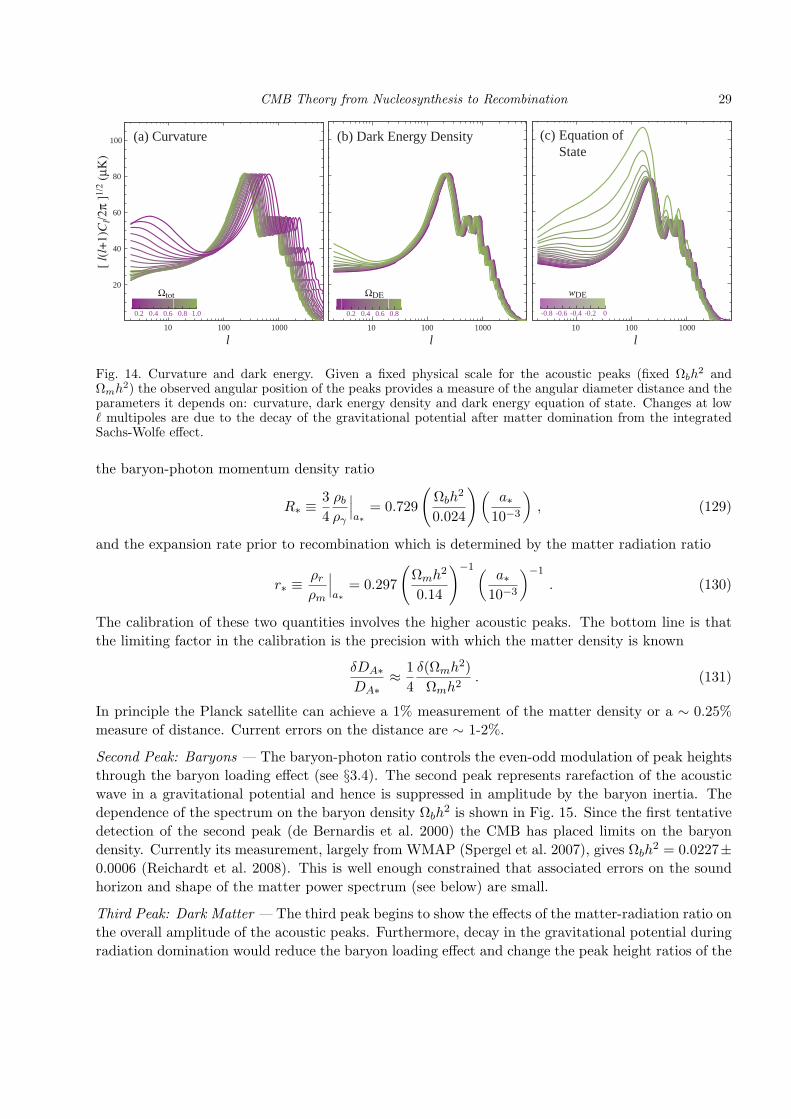
Fig. 14. Curvature and dark energy. Given a fixed physical scale for the acoustic peaks (fixed Ωbh2 andΩmh2) the observed angular position of the peaks provides a measure of the angular diameter distance and theparameters it depends on: curvature, dark energy density and dark energy equation of state. Changes at low` multipoles are due to the decay of the gravitational potential after matter domination from the integratedSachs-Wolfe effect.

the baryon-photon momentum density ratio

R∗ ≡34ρbργ

∣∣∣a∗

= 0.729

(Ωbh

2

0.024

)(a∗

10−3

), (129)

and the expansion rate prior to recombination which is determined by the matter radiation ratio

r∗ ≡ρrρm

∣∣∣a∗

= 0.297

(Ωmh

2

0.14

)−1 (a∗

10−3

)−1

. (130)

The calibration of these two quantities involves the higher acoustic peaks. The bottom line is thatthe limiting factor in the calibration is the precision with which the matter density is known

δDA∗DA∗

≈ 14δ(Ωmh

2)Ωmh2

. (131)

In principle the Planck satellite can achieve a 1% measurement of the matter density or a ∼ 0.25%measure of distance. Current errors on the distance are ∼ 1-2%.

Second Peak: Baryons — The baryon-photon ratio controls the even-odd modulation of peak heightsthrough the baryon loading effect (see §3.4). The second peak represents rarefaction of the acousticwave in a gravitational potential and hence is suppressed in amplitude by the baryon inertia. Thedependence of the spectrum on the baryon density Ωbh

2 is shown in Fig. 15. Since the first tentativedetection of the second peak (de Bernardis et al. 2000) the CMB has placed limits on the baryondensity. Currently its measurement, largely from WMAP (Spergel et al. 2007), gives Ωbh

2 = 0.0227±0.0006 (Reichardt et al. 2008). This is well enough constrained that associated errors on the soundhorizon and shape of the matter power spectrum (see below) are small.

Third Peak: Dark Matter — The third peak begins to show the effects of the matter-radiation ratio onthe overall amplitude of the acoustic peaks. Furthermore, decay in the gravitational potential duringradiation domination would reduce the baryon loading effect and change the peak height ratios of the

30

10

0.02 0.04 0.06

100 1000

20

40

60

80

100

l10 100 1000

l

0.1 0.2 0.3 0.4 0.5

(a) Baryons (b) Matter

Fig. 15. Baryons and matter. Baryons change the relative heights of the even and odd peaks through theirinertia in the plasma. The matter-radiation ratio also changes the overall amplitude of the oscillations fromdriving effects. Adapted from Hu and Dodelson (2002).

second and third peaks (e.g. Hu et al. 2001). The dependence of the spectrum on the baryon densityΩmh

2 is shown in Fig. 15. Constraints on the third peak from the DASI experiment (Pryke et al.2001) represented the first direct evidence for dark matter at the epoch of recombination. Currentconstraints from a combination of WMAP and higher resolution ground and balloon based data yieldΩmh

2 = 0.135 ± 0.007 (Reichardt et al. (2008)). Since this parameter controls the error on thedistance to recombination through equation (131) and the matter power spectrum (see below), it isimportant to improve the precision of its measurement with the third higher peaks.

Damping Tail: Consistency— Under the standard thermal history of §2 and matter content, theparameters that control the first 3 peaks also determine the structure of the damping tail at ` > 103:namely, the angular diameter distance to recombination D∗, the baryon density Ωbh

2 and the matterdensity Ωmh

2. When the damping tail was first discovered by the CBI experiment (Padin et al. 2001),it supplied compelling support for the standard theoretical modeling of the physics at recombinationoutlined here. Currently the best constraints on the damping tail are from the ACBAR experiment(Reichardt et al. 2008, see Fig. 7). Consistency between the low order peaks and the damping tailcan be used to make precision tests of recombination and any physics beyond the standard model atthat epoch. For example, damping tail measurements can be used to constrain the evolution of thefine structure constant.

Matter Power Spectrum: Shape & Amplitude — The acoustic peaks also determine the shape andamplitude of the matter power spectrum. Firstly, acoustic oscillations are shared by the baryons. Inparticular, the plasma motion kinematically produces enhancements of density near recombination(see Eqn. 113))

δb ≈ −kη∗vb(η∗) ≈ −kη∗vγ(η∗) . (132)

This enhancement then imprints into the matter power spectrum at an amplitude reduced by ρb/ρmdue to the small baryon fraction (Hu and Sugiyama 1996). Secondly, the gravitational potentialsthat the cold dark matter perturbations fall in are evolving through the plasma epoch due to the


1

0.1

0.0001 0.001 0.01 0.1 10.01

T(k

)

k (h Mpc-1 )

baryonoscillations

equalityk-2

Fig. 16. Transfer function. Acoustic and radiation physics is imprinted on the matter power spectrum asquantified by the transfer function T (k). The former is responsible for baryon oscillations in the spectrum andthe latter a suppression of growth due to Jeans stability for scales smaller than the horizon at matter-radiationequality.

processes described in §3.5. On scales above the horizon, relativistic stresses are never important andthe gravitational potential remains constant. The Poisson equation then implies that

∆ ∼ (kη)2Φ(0) , (133)

and in particular, the density perturbation at horizon crossing where kη ∼ 1 is ∆ = ∆H ≈ Φ(0). Fora fluctuation that crosses the horizon during radiation domination, the total density perturbation isJeans stabilized until matter radiation equality

ηeq ≈ 114

(Ωmh

2

0.14

)−1

Mpc . (134)

Thereafter, relativistic stresses again become irrelevant and the potential remains unchanged untilmatter ceases to dominate the expansion

Φ ≈ (kηeq)−2∆H ∼ (kηeq)−2Φ(0) . (135)

The transfer in shape from the initial conditions due to baryon oscillations and matter radiationequality is usually encapsulated into a transfer function T (k). Given an initial power spectrum ofthe form (94), the evolution through to matter domination transforms the potential power spectrumto k3PΦ/2π2 ∝ kn−1T 2(k) where T (k) ∝ k−2 beyond the wavenumber at matter-radiation equality.This scaling is slightly modified due to the logarithmic growth of dark matter fluctuations during theradiation epoch when the radiation density is Jeans stable. The matter power spectrum and potentialpower spectrum are related by the Poisson equation and so carry the same shape. Specifically

k3Pm(k, a)2π2

=425δ2ζ

(G(a)a

Ωm

)2 ( k

H0

)4 ( k

knorm

)n−1

T 2(k) , (136)

where we have included a factor G(a) to account for the decay in the potential during the acceleration

32

epoch when relativistic stresses are again important (see e.g. Hu (2005)). This factor only dependson time and not scale as long as the scale in question is within the Jeans scale of the acceleratingcomponent. In this limit, G(a) is determined by the solution to

d2G

d ln a2+(

4 +d lnHd ln a

)dG

d ln a+[3 +

d lnHd ln a

− 32

Ωm(a)]G = 0 , (137)

with an initial conditions of G(ln amd) = 1 and G′(ln amd) = 0 at an epoch amd when the universe isfully matter dominated.

The transfer function T (k), with k in Mpc−1, depends only on the baryon density Ωbh2 and

the matter density Ωmh2 which are well determined by the CMB acoustic peaks. Features in the

matter power spectrum, especially the baryon oscillations, then serve as standard rulers for distancemeasurements Eisenstein et al. (1998). For example, its measurement in a local redshift survey wherethe distance is calibrated in h Mpc−1 would give the Hubble constant h. Detection of the featuresrequires a Gpc3 of volume and so precise, purely local, measurements are not feasible. Nonetheless,the first detection of these oscillations by the SDSS LRG redshift survey out to z ∼ 0.4 provideremarkably tight constraints on the acceleration of the expansion (Eisenstein et al. 2005).

The CMB also determines the initial normalization δζ and so provides a means by which to test theeffect of the acceleration on the growth functionG(a). The precision of this determination is largely setby reionization. The opacity provided by electrons after reionization suppress the observed amplitudeof the peaks relative to the initial amplitude and hence

δζ ≈ 4.6e−(0.1−τ) × 10−5 , (138)

where τ is the optical depth to recombination. Note that this is the normalization at k = 0.05 Mpc−1

and even with uncertainties in the optical depth of δτ ∼ 0.03 it exceeds the precision of the COBEnormalization (c.f. Eqn. (95)). Finally, with the matter and baryon transfer effects determined, theacoustic spectrum also constrains the tilt. WMAP provided the first hints of a small deviation fromscale invariance (Spergel et al. 2007) and the current constraints are n ≈ 0.965± 0.015.

Combining these factors into the conventional measure of the amplitude of matter fluctuationstoday

σ28 ≡

∫dk

k

k3P (k, a = 1)2π2

W 2σ (kr)

σ8 ≈ δζ5.59× 10−5

(Ωbh

2

0.024

)−1/3(Ωmh

2

0.14

)0.563

×(3.123h)(n−1)/2(

h

0.72

)0.693 G0

0.76, (139)

where Wσ(x) = 3x−3(sinx − x cosx) is the Fourier transform of a top hat window of radius r =8h−1Mpc.

4 Polarization Anisotropy from Recombination

Thomson scattering of quadrupolarly anisotropic but unpolarized radiation generates linear polar-ization. As we have seen in §3.1, ` ≥ 2 anisotropy develops only in optically thin conditions. Giventhat polarization also requires scattering to be generated, the polarization anisotropy is genericallymuch smaller than the temperature anisotropy. The main source of polarization from recombination


0 500 1000 1500 2000 2500l

-50

0

50

100

150

l(l+

1)C

l / 2π

(μK

2 )

MAXIPOLDASICBIBOOMERanGWMAPQUaDCAPMAP

Fig. 17. E-mode polarization power spectrum measurements. Adapted from Bischoff et al. (2008).

is associated with the acoustic peaks in temperature. This source was first detected by the DASIexperiment (Kovac et al. 2002) and recent years have seen increasingly precise measurements (seeFig. 17).

Since acoustic polarization arises from linear scalar perturbations, they possess a symmetry thatrelates the direction of polarization to the wavevector or change in the polarization amplitude. As weeshall see in the next section, this symmetry is manifest in the the absence of B-modes (Kamionkowskiet al. 1997; Zaldarriaga and Seljak 1997). B-modes at recombination can be generated from thequadrupole moment of a gravitational wave. This yet-to-be-detected signal would be invaluable forearly universe studies involving the inflationary origin of perturbations.

We begin by reviewing the Stokes parameter description of polarization (§4.1) and its relationto E and B harmonic representation (§4.2). We continue with a discussion of polarized Thomsonscattering in §4.3. In §4.4 and 4.5 we discuss the polarization signatures of acoustic oscillations andgravitational waves.

4.1 Statistical Description

The polarization field can be analyzed in a way very similar to the temperature field, save for onecomplication. In addition to its strength, polarization also has an orientation, depending on relativestrength of two linear polarization states.

The polarization field is defined locally in terms of Stokes parameters. In general, the polarizationstate of radiation in direction n described by the intensity matrix

⟨Ei(n)E∗j (n)

⟩, where E is the

electric field vector in the transverse plane and the brackets denote time averaging. As a 2 × 2hermitian matrix, it can be decomposed into the Pauli basis

P = C⟨E(n) E†(n)

⟩= Θ(n)σ0 +Q(n) σ3 + U(n) σ1 + V (n) σ2 , (140)

34

where

σ0 =

(1 00 1

), σ2 =

(0 −11 0

)i ,

σ1 =

(0 11 0

), σ3 =

(1 00 −1

). (141)

Orthogonality of the Pauli matrices says that the Stokes parameters are recovered from the polariza-tion matrix as Tr(σiP)/2. The Stokes Q and U parameter define the linear polarization state whereasV defines the circular polarization state. We have chosen the proportionality constant so that all theStokes parameters are in temperature fluctuation units.

From this description, we see that Q represents polarization aligned with one of the principal axesof the transverse coordinate system whereas U represents polarization at 45 to these axes.

4.2 EB Harmonic Description

The disadvantage of the Stokes Q and U representation is that the distinction between the twodepends on the coordinate system for the two transverse directions on the sky. Under a rotation ofthis basis by θ

Q′ ± iU ′ = e∓2iθ[Q± iU ] . (142)

For a harmonic decomposition, it is more useful to choose this basis to be given by the wavevectoritself. For small sections of the sky, the harmonic decomposition becomes a Fourier transform andwe can define the E and B harmonics as

E(l)± iB(l) =∫dn[Q′(n)± iU ′(n)]e−il·n (143)

= e∓2iφl

∫dn[Q(n)± iU(n)]e−il·n ,

where in the second line we have rotated Q and U back to a fixed coordinate system with the angleφl that the Fourier vector makes with the x axis.

For linear scalar fluctuations, we have seen that the only direction for a given harmonic mode isset by the direction of the wavevector itself: velocity fields point in this direction or its opposite,quadrupole moments are symmetric about this axis, etc. This means that symmetry requires thatsuch sources only generate Q′ or E for each mode. This symmetry also holds once all the modesare superimposed back to the full polarization field: linear scalar perturbations generate only E-modes where the polarization direction is related to the direction in which the polarization amplitudechanges.

To generalize this decomposition to the full curved sky, we need to replace plane waves, the tensoreigenfunctions of the Laplace operator in a flat space, to the correct tensor eigenfunctions for thecurved space. These are called the spin-2 spherical harmonics:

∇2±2Y`m[σ3 ∓ iσ1] = −[l(l + 1)− 4]±2Y`m[σ3 ∓ iσ1] . (144)

They obey the usual orthogonality and completeness relations∫dnsY ∗`m(n)sY`m(n) = δ``′δmm′ ,∑`m

sY∗`m(n)sY`m(n′) = δ(φ− φ′)δ(cos θ − cos θ′) . (145)


Thomson Scattering

E1

E1

E2

E2

e-

’

’

Fig. 18. Thomson scattering geometry. A quadrupole anisotropy in the incoming radiation leads to linearpolarization. For scattering at Θ = π/2, only one component of the initially unpolarized radiation (E′2) isscattered leaving one outgoing state (E1) unpopulated.

We can therefore decompose the linear polarization field just like the temperature field

[Q(n)± iU(n)] = −∑`m

[E`m ± iB`m]±2Y`m(n) . (146)

Likewise the power spectra are given by

〈E∗`mE`m〉 = δ``′δmm′CEE` , (147)

〈B∗`mB`m〉 = δ``′δmm′CBB` , (148)

and the cross correlation of E-polarization with temperature by

〈Θ∗`mE`m〉 = δ``′δmm′CΘE` . (149)

Other cross correlations vanish if parity is conserved.

4.3 Thomson Scattering

The differential cross section for Thomson scattering

dσ

dΩ=

38π|E′ · E|2σT , (150)

is polarization dependent and hence scattering generates polarization. Here E′ and E denote theincoming and outgoing directions of the electric field or polarization vector. Consider incomingradiation in the x direction scattered at right angles into the −y direction (see Fig. 18). Heuristically,incoming radiation shakes an electron in the direction of its electric field vector or polarization e′

causing it to radiate with an outgoing polarization parallel to that direction. However since theoutgoing polarization e must be orthogonal to the outgoing direction, incoming radiation that ispolarized parallel to the outgoing direction cannot scatter leaving only one polarization state.

The incoming radiation however comes from all angles. If it were completely isotropic in intensity,radiation coming along the z would provide the polarization state that is missing from that comingalong x leaving the net outgoing radiation unpolarized. Only a quadrupole temperature anisotropyin the radiation generates a net linear polarization from Thomson scattering. As we have seen, aquadrupole can only be efficiently generated if the universe is optically thin to Thomson scattering agiven perturbation.

36

100

10

10 100 1000

1

0.1

0.01

l (multipole)

reionization

dark energy

gravitationalwaves

gravitationallensing

EE

BB

curvature, baryons, dark matter

Fig. 19. Polarized landscape. While the E-spectrum and ΘE cross correlation are increasingly well measured,the B-spectrum from inflationary gravitational waves (shown here near the maximal value allowed by thetemperature spectrum) and gravitational lensing remains undetected. Shown here are projected error barsassociated with Planck sample variance and detector noise. Adapted from Hu and Dodelson (2002).

4.4 Acoustic Polarization

Acoustic oscillations in the dissipation regime provide the conditions necessary for polarization. Recallthat radiative viscosity in the plasma is equivalent to quadrupole anisotropy in the photons. Sincethe quadrupole is of order (see Fig. 11)

πγ ∼kvγτ∼(k

kD

)vγkDη∗

, (151)

the polarization spectrum rises as l/lD to peak at the damping scale with an amplitude of about 10%of the temperature fluctuations before falling due to the elimination of the acoustic source itself dueto damping. Since vγ is out of phase with the temperature,

Θ + Ψ ∝ cos(ks); vγ ∝ sin(ks) , (152)

the polarization peaks are also out of phase with the temperature peaks. Furthermore, the phaserelation also tells us that the polarization is correlated with the temperature perturbations. The cor-relation power CΘE

l being the product of the two, exhibits oscillations at twice the acoustic frequency

(Θ + Ψ)(vγ) ∝ cos(ks) sin(ks) ∝ sin(2ks) . (153)

As in the case of the damping, the predicting the precise value requires numerical codes (Bond andEfstathiou 1987) since τ changes so rapidly near recombination. Nonetheless the detailed predictionsbear these qualitative features.

Like the damping scale, the acoustic polarization spectrum is uniquely predicted from the temper-ature spectrum once Ωbh

2, Ωmh2 and the initial conditions are specified. Polarization thus represents


a sharp test on the assumptions of the recombination physics and power law curvature fluctuations inthe initial conditions used in interpreting the temperature peaks. For example, features in the initialpower spectrum appear more distinct in the polarization than the temperature due to projectioneffects (see e.g. Hu and Okamoto (2004)).

4.5 Gravitational Waves

During the break down of tight coupling that occurs at last scattering, any gravitational wavespresent will also imprint a local quadrupole anisotropy to the photons and hence a linear polarizationto the CMB (Polnarev 1985). These contribute to the BB power and their detection would provideinvaluable information on the origin of the fluctuations. Specifically, in simple inflationary modelstheir amplitude gives the energy scale of inflation. The gravitational wave amplitude h oscillates anddecays once inside the horizon, so the associated polarization source scales as h/τ and so peaks atthe l ≈ 100 horizon scale and not the damping scale at recombination (see Fig. 19). This provides auseful scale separation of the various polarization effects.

If the energy scale of inflation is near the 1016GeV scale then the signal is potentially detectableby the next generation of polarization experiments.

5 Discussion

The one and a half decades since the discovery of CMB anisotropy by COBE DMR has seen re-markable progress that ushered in the current epoch of precision cosmology. From the preliminarydetections of degree scale power to the current measurements of 5 acoustic peaks, the damping tail andacoustic polarization, the milestones in the observational verification of our theoretical understandingof the universe at recombination have steadily been overtaken. Correspondingly, the measurementsof the energy density contents of the universe at recombination and the distance to and hence ex-pansion rate since recombination have improved from order unity constraints to several percent leveldeterminations.

The next generation of experiments, including the Planck satellite and ground based polarizationmeasurements, will push these determinations to the 1% level and beyond and perhaps detect the oneoutstanding prediction of the recombination epoch: the B-mode polarization of gravitational wavesfrom inflation. Likewise the enhanced range of precision measurements of the power spectrum willbring measurements of the spectrum of scalar perturbations to the percent level and further test thephysics of inflation.

Beyond the recombination epoch reviewed here, these experiments will also test secondary tem-perature and polarization anisotropy from reionization, lensing, and galaxy clusters as well as theGaussianity of the initial conditions. Combined, these measurements will test the standard cosmo-logical model with unprecedented precision.

Acknowledgments: I thank the organizers, R. Rebelo and J.A. Rubino-Martin, as well as the studentsof the XIX Canary Island Winter School of Astrophysics.

ReferencesAlpher, R.A. and Herman, R.C. (1948). On the relative abundance of the elements, Phys. Rev., 74, 1737–1742.Bardeen, J.M. (1980). Gauge invariant cosmological perturbations, Phys. Rev., D22, 1882–1905.

38

Bischoff, C. et al. (2008). New Measurements of Fine-Scale CMB Polarization Power Spectra from CAPMAPat Both 40 and 90 GHz. arXiv:0802.0888 [astro-ph].

Bond, J.R. and Efstathiou, G. (1984). Cosmic background radiation anisotropies in universes dominated bynonbaryonic dark matter, Astrophys. J. Lett., 285, L45–L48.

Bond, J.R. and Efstathiou, G. (1987). The statistics of cosmic background radiation fluctuations, Mon. Not.R. Astron. Soc., 226, 655–687.

Danese, L. and de Zotti, G. (1982). Double Compton process and the spectrum of the microwave background,Astron. Astrophys., 107, 39–42.

de Bernardis, P. et al. (2000). A flat Universe from high-resolution maps of the cosmic microwave backgroundradiation, Nature, 404, 955–959.

Dicke, R.H., Peebles, P.J.E., Roll, P.G. and Wilkinson, D.T. (1965). Cosmic Black-Body Radiation., Astrophys.J., 142, 414–419.

Eisenstein, D.J. et al. (2005). Detection of the Baryon Acoustic Peak in the Large-Scale Correlation Functionof SDSS Luminous Red Galaxies, Astrophys. J., 633, 560–574. astro-ph/0501171.

Eisenstein, D., Hu, W. and Tegmark, M. (1998). Cosmic Complementarity: H0 and Ωm from Combining CMBExperiments and Redshift Surveys, Astrophys. J. Lett., 504, L57. astro-ph/9805239.

Fixsen, D.J. et al. (1996). The Cosmic Microwave Background Spectrum from the Full COBE FIRAS DataSet, Astrophys. J., 473, 576–587.

Gamow, G. (1948). The origin of elements and the separation of galaxies, Phys. Rev., 74, 505–506.Hanany, S. et al. (2000). MAXIMA-1: A Measurement of the Cosmic Microwave Background Anisotropy on

Angular Scales of 10’-5°, Astrophys. J. Lett., 545, L5–L9.Hu, W. (2003). Covariant Linear Perturbation Formalism, ICTP, 14, 149. astro-ph/0402060.Hu, W. (2005). Dark Energy Probes in Light of the CMB, ASPC, 339, 215. astro-ph/0407158.Hu, W. and White, M.J. (2004). The cosmic symphony, Sci. Am., 290N2, 32–37.Hu, W. (1995). Wandering in the background: A Cosmic microwave background explorer. astro-ph/9508126.Hu, W. and Dodelson, S. (2002). Cosmic Microwave Background Anisotropies, Ann. Rev. Astron. Astrophys.,

40, 171–216. astro-ph/0110414.Hu, W., Fukugita, M., Zaldarriaga, M. and Tegmark, M. (2001). CMB Observables and Their Cosmological

Implications, Astrophys. J., 549, 669. astro-ph/0006436.Hu, W. and Okamoto, T. (2004). Principal Power of the CMB, Phys. Rev., D69, 043004. astro-ph/0308049.Hu, W. and Silk, J. (1993). Thermalization and spectral distortions of the cosmic background radiation, Phys.

Rev., D48, 485–502.Hu, W. and Sugiyama, N. (1995). Anisotropies in the Cosmic Microwave Background: An Analytic Approach,

Astrophys. J., 444, 489–506. astro-ph/9407093.Hu, W. and Sugiyama, N. (1996). Small scale cosmological perturbations: An Analytic approach, Astrophys.

J., 471, 542–570. astro-ph/9510117.Hu, W. and White, M.J. (1996). A New Test of Inflation, Phys. Rev. Lett., 77, 1687–1690. astro-ph/9602020.Hu, W. and White, M.J. (1997). CMB Anisotropies: Total Angular Momentum Method, Phys. Rev., D56,

596–615. astro-ph/9702170.Kaiser, N. (1983). Small-angle anisotropy of the microwave background radiation in the adiabatic theory, Mon.

Not. R. Astron. Soc., 202, 1169–1180.Kamionkowski, M., Kosowsky, A. and Stebbins, A. (1997). Statistics of cosmic microwave background polar-

ization, Phys. Rev., D55, 7368–7388. astro-ph/9611125.Kovac, J. et al. (2002). Detection of polarization in the cosmic microwave background using DASI, Nature,

420, 772–787. astro-ph/0209478.Lewis, A., Challinor, A. and Lasenby, A. (2000). Efficient Computation of Cosmic Microwave Background

Anisotropies in Closed Friedmann-Robertson-Walker Models, Astrophys. J., 538, 473–476. arXiv:astro-ph/9911177.

Mather, J.C., Fixsen, D.J., Shafer, R.A., Mosier, C. and Wilkinson, D.T. (1999). Calibrator Design for theCOBE Far Infrared Absolute Spectrophotometer (FIRAS), Astrophys. J., 512, 511–520. astro-ph/9810373.

Miller, A.D. et al. (1999). A Measurement of the Angular Power Spectrum of the Cosmic Microwave Backgroundfrom L = 100 to 400, Astrophys. J. Lett., 524, L1–L4.

Padin, S. et al. (2001). First Intrinsic Anisotropy Observations with the Cosmic Background Imager, Astrophys.J. Lett., 549, L1–L5.

Peebles, P.J.E. (1968). Recombination of the Primeval Plasma, Astrophys. J., 153, 1–11.Peebles, P.J.E. and Yu, J.T. (1970). Primeval Adiabatic Perturbation in an Expanding Universe, Astrophys.

J., 162, 815–836.


Polnarev, A.G. (1985). Polarization and Anisotropy Induced in the Microwave Background by CosmologicalGravitational Waves, Soviet Astronomy, 29, 607–+.

Pryke, C. et al. (2001). Cosmological Parameter Extraction from the First Season of Observations with DASI,Astrophys. J., In Press. astro-ph/0104490.

Reichardt, C.L. et al. (2008). High resolution CMB power spectrum from the complete ACBAR data set.arXiv:0801.1491 [astro-ph].

Sachs, R.K. and Wolfe, A.M. (1967). Perturbations of a Cosmological Model and Angular Variations of theMicrowave Background, Astrophys. J., 147, 73–90.

Seager, S., Sasselov, D.D. and Scott, D. (2000). How exactly did the Universe become neutral?, Astrophys. J.Suppl., 128, 407–430. astro-ph/9912182.

Seljak, U. and Zaldarriaga, M. (1996). A Line-of-Sight Integration Approach to Cosmic Microwave BackgroundAnisotropies, Astrophys. J., 469, 437–444.

Silk, J. (1968). Cosmic Black-Body Radiation and Galaxy Formation, Astrophys. J., 151, 459–471.Smoot, G.F. et al. (1992). Structure in the COBE differential microwave radiometer first-year maps, Astrophys.

J. Lett., 396, L1–L5.Spergel, D.N. et al. (2007). Wilkinson Microwave Anisotropy Probe (WMAP) three year results: Implications

for cosmology, Astrophys. J. Suppl., 170, 377. astro-ph/0603449.Switzer, E.R. and Hirata, C.M. (2007). Primordial helium recombination III: Thomson scattering, isotope

shifts, and cumulative results. astro-ph/0702145.Tytler, D. et al. (2000). Review of Big Bang nucleosynthesis and primordial abundances., Physica Scripta

Volume T, 85, 12–31.Vittorio, N. and Silk, J. (1984). Fine-scale anisotropy of the cosmic microwave background in a universe

dominated by cold dark matter, Astrophys. J. Lett., 285, L39–L43.White, M.J. and Hu, W. (1997). The Sachs-Wolfe effect, Astron. Astrophys., 321, 8–9. astro-ph/9609105.Wong, W.Y., Moss, A. and Scott, D. (2007). How well do we understand cosmological recombination?

arXiv:0711.1357 [astro-ph].Zaldarriaga, M. and Seljak, U. (1997). An all-sky analysis of polarization in the microwave background, Phys.

Rev. D, 55, 1830–1840. astro-ph/9609170.Zeldovich, Y.B. and Sunyaev, R.A. (1969). The Interaction of Matter and Radiation in a Hot-Model Universe,

Astrophys. Space Sci., 4, 301–316.

Documents

0802.3688