08 Numisheet2008 Hot Forming Chapter8

Chapter 8

Hot Forming

Numisheet 2008 September 1 - 5, 2008 – Interlaken, Switzerland

Figure 5: Comparison of experimental and FE sim-ulation results for springback in metal strips subjectto draw-bending (r=15mm)

tional shell elements. For efficiency, the symmetryof the strip (Figure 3) has been exploited in the sim-ulation. The minimal friction taking place betweenthe roller and strip has been modelled in ABAQUSvia the definition of a ”Contact Property” of ”Fric-tion” type. A comparison of the simulation and ex-perimental results for springback of the strip usingrollers of diameter 10 mm and 15 mm are shown inFigure 4 and Figure 5. The agreement between theseis very good in the case of the combined hardeningmodeling. For comparison, simulation results basedon models for purely isotropic and purely kinematichardening are also shown for the 10 mm case in Fig-ure 4. As shown, the purely isotropic model resultsin an overestimate, and the purely kinematic modelin an underestimate, of the amount of springback. Inparticular, note that the purely isotropic model un-derestimates the amount of inelastic deformation. Inorder to satisfy the boundary conditions, then, theamount of elastic deformation is overestimated, re-sulting in too much springback. Similar results havebeen obtained for other types of steels, e.g., DP 600[3].

5 CONCLUSIONS

Using the tension-compression test results, modelsfor purely isotropic, purely kinematic, and com-bined hardening have been identified for the newsteel LH800. The identified model was validatedwith the help of the finite-element simulation ofdraw-bending. The deep drawing process is work inprogress which will be presented at the conference.This holds for the experiments and the simulations.In particular spring-back and distortional hardening

will be included in the FE-simulations.

6 ACKNOWLEDGEMENTFinancial support for this work was provided by theGerman National Science Foundation (DFG) underthe contract SV 8/9-1 in the priority program 1204and is gratefully acknowledged.

REFERENCES[1] J. Wang, V. Levkovitch, F. Reusch,

B. Svendsen, J. Hueting, and M. Van Reel. Onthe modeling of hardening in metals duringnon-proportional loading. In InternationalJournal of Plasticity 24, pages 1039–1070,2008.

[2] V. Levkovitch and B. Svendsen. Accuratehardening modeling as basis for the realisticsimulation of sheet forming processes withcomplex strain-path changes. In Proceedings ofthe 9th international Conference on NumericalMethods in Industrial Forming Processes,pages 1331–1336, 2007, Porto.

[3] J. Wang, V. Levkovitch, F. Reusch, andB. Svendsen. On the modeling and simulationof induced anisotropy in polycrystalline metalswith application to springback. In Archive ofApplied Mechanics 74, pages 890–899, 2005.

551


____________________ * Corresponding author: AUDI Ingolstadt, [email protected]

SIMULATION IN TOOL AND DIE SHOP

B. Griesbach*1, B. Oberpriller1

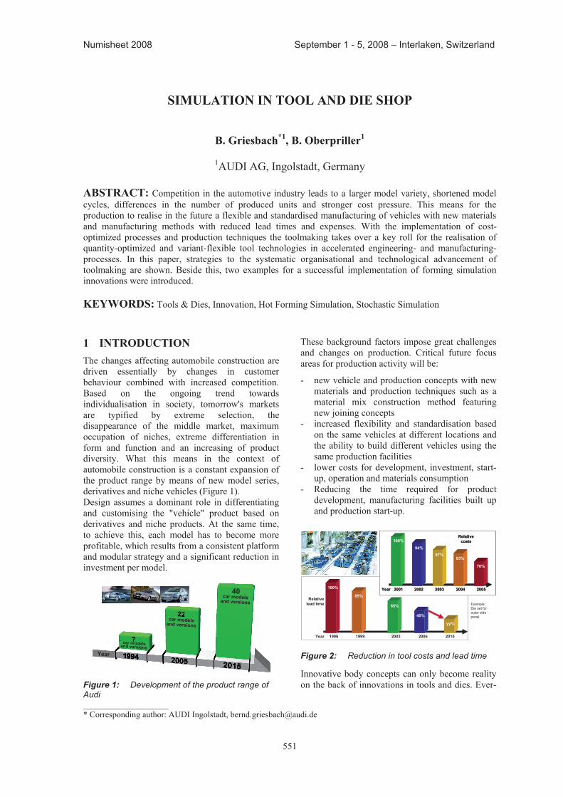
1AUDI AG, Ingolstadt, Germany ABSTRACT: Competition in the automotive industry leads to a larger model variety, shortened model cycles, differences in the number of produced units and stronger cost pressure. This means for the production to realise in the future a flexible and standardised manufacturing of vehicles with new materials and manufacturing methods with reduced lead times and expenses. With the implementation of cost-optimized processes and production techniques the toolmaking takes over a key roll for the realisation of quantity-optimized and variant-flexible tool technologies in accelerated engineering- and manufacturing-processes. In this paper, strategies to the systematic organisational and technological advancement of toolmaking are shown. Beside this, two examples for a successful implementation of forming simulation innovations were introduced. KEYWORDS: Tools & Dies, Innovation, Hot Forming Simulation, Stochastic Simulation 1 INTRODUCTION The changes affecting automobile construction are driven essentially by changes in customer behaviour combined with increased competition. Based on the ongoing trend towards individualisation in society, tomorrow's markets are typified by extreme selection, the disappearance of the middle market, maximum occupation of niches, extreme differentiation in form and function and an increasing of product diversity. What this means in the context of automobile construction is a constant expansion of the product range by means of new model series, derivatives and niche vehicles (Figure 1). Design assumes a dominant role in differentiating and customising the "vehicle" product based on derivatives and niche products. At the same time, to achieve this, each model has to become more profitable, which results from a consistent platform and modular strategy and a significant reduction in investment per model.

40car models and versions

car models and versions

car models and versionsYear

Figure 1: Development of the product range of Audi

These background factors impose great challenges and changes on production. Critical future focus areas for production activity will be:

- new vehicle and production concepts with new materials and production techniques such as a material mix construction method featuring new joining concepts

- increased flexibility and standardisation based on the same vehicles at different locations and the ability to build different vehicles using the same production facilities

- lower costs for development, investment, start-up, operation and materials consumption

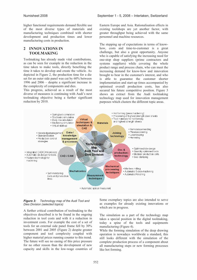
- Reducing the time required for product development, manufacturing facilities built up and production start-up.

Relative lead time

100%

1996 1999 2003 2006

85%

65%

40%

Year

Relative costs100%

2001 2002 2004 2005

94%

83%

70%

Year

87%

2003

Relative costs100%

2001 2002 2004 2005

94%

83%

70%

Year

87%

2003

Relative costs100%

2001 2002 2004 2005

94%

83%

70%

Year

87%

2003

Example: Die set for outer side panel

2010

yy%

Figure 2: Reduction in tool costs and lead time

Innovative body concepts can only become reality on the back of innovations in tools and dies. Ever-

552


higher functional requirements demand flexible use of the most diverse types of materials and manufacturing techniques combined with shorter development and production times and lower manufacturing costs in production. 2 INNOVATIONS IN

TOOLMAKING Toolmaking has already made vital contributions, as can be seen for example in the reduction in the time taken to make tools, directly benefiting the time it takes to develop and create the vehicle. As depicted in Figure 2, the production time for a die set for an outer side panel was cut by 60% between 1996 and 2006 – despite a significant increase in the complexity of components and dies. This progress, achieved as a result of the most diverse of measures is continuing with Audi’s next toolmaking objective being a further significant reduction by 2010.

Figure 3: Technology map of the Audi Tool and Dies Division (selected topics)

A further critical contribution of toolmaking to the objectives described is to be found in the ongoing reduction in tool costs and with it a reduction in investment costs. For example the cost of a set of tools for an external side panel frame fell by 30% between 2001 and 2005 (Figure 2) despite greater component and tool complexity coupled with higher material prices running counter to this trend. The future will see no easing of this price pressure for no other reason than the development of new capacity and skills in the low-wage countries of

Eastern Europe and Asia. Rationalisation effects in existing toolshops are yet another factor, with greater throughput being achieved with the same personnel and machine resources. The stepping up of expectations in terms of know-how, costs and time-to-customer is a great challenge, but also a great opportunity. Anyone who is capable of satisfying the increasing need for one-stop shop suppliers (prime contractors and systems suppliers) while covering the whole product range and process chain, who can meet the increasing demand for know-how and innovation brought to bear in the customer's interest, and who is able to guarantee the customer shorter implementation and start-up times accompanied by optimised overall production costs, has also secured his future competitive position. Figure 3 shows an extract from the Audi toolmaking technology map used for innovation management purposes which clusters the different topic areas.

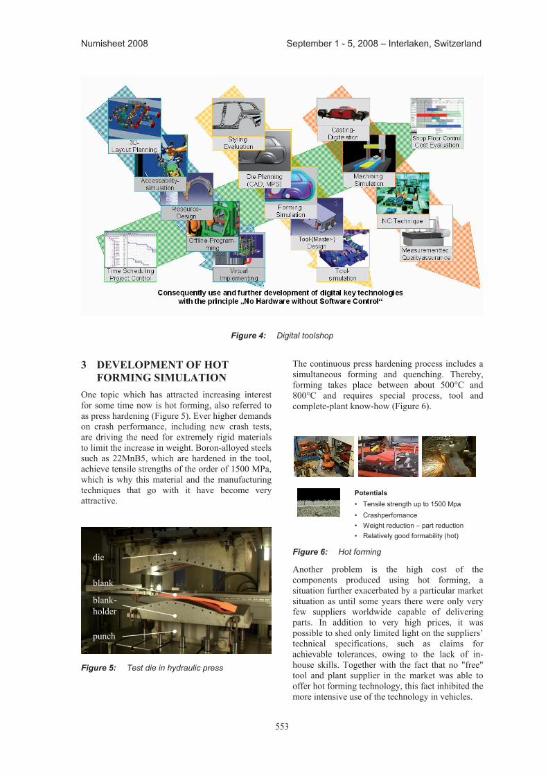
Some exemplary topics are also intended to serve as examples for already existing innovations or which are in progress. The simulation as a part of the technology map takes a special position in the digital toolmaking, today a spine of the tools and equipments manufacturing (Figure 4). While the forming simulation of the deep drawing operation is nowadays worldwide a standard, this still looks different with the simulation of the complete production process of a component about all manufacturing steps or new forming processes like hot forming.

553


Figure 4: Digital toolshop

3 DEVELOPMENT OF HOT

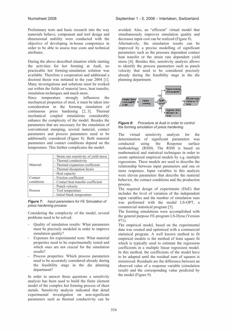
FORMING SIMULATION One topic which has attracted increasing interest for some time now is hot forming, also referred to as press hardening (Figure 5). Ever higher demands on crash performance, including new crash tests, are driving the need for extremely rigid materials to limit the increase in weight. Boron-alloyed steels such as 22MnB5, which are hardened in the tool, achieve tensile strengths of the order of 1500 MPa, which is why this material and the manufacturing techniques that go with it have become very attractive.

Figure 5: Test die in hydraulic press

The continuous press hardening process includes a simultaneous forming and quenching. Thereby, forming takes place between about 500°C and 800°C and requires special process, tool and complete-plant know-how (Figure 6).

Figure 6: Hot forming

Another problem is the high cost of the components produced using hot forming, a situation further exacerbated by a particular market situation as until some years there were only very few suppliers worldwide capable of delivering parts. In addition to very high prices, it was possible to shed only limited light on the suppliers’ technical specifications, such as claims for achievable tolerances, owing to the lack of in-house skills. Together with the fact that no "free" tool and plant supplier in the market was able to offer hot forming technology, this fact inhibited the more intensive use of the technology in vehicles.

die

punch

blankholder

blank

Potentials• Tensile strength up to 1500 Mpa• Crashperfomance• Weight reduction – part reduction• Relatively good formability (hot)

554


Preliminary tests and basic research into the way materials behave; component and tool design and dimensional stability were conducted with the objective of developing in-house competence in order to be able to assess true costs and technical attributes. During the above described situation while starting the activities for hot forming at Audi, no practicable hot forming-simulation solution was available. Therefore a cooperation and additional a doctoral thesis was initiated in the year 2004 [1]. Many investigations and solutions must be worked out within the fields of material laws, heat transfer, simulation techniques and much more. Since temperature strongly influences the mechanical properties of steel, it must be taken into consideration in the forming simulation of continuous press hardening [2, 3]. Thermal mechanical coupled simulations considerably enhance the complexity of the model. Besides the parameters that are necessary for the simulation of conventional stamping, several material, contact parameters and process parameters need to be additionally considered (Figure 8). Both material parameters and contact conditions depend on the temperature. This further complicates the model.

- Strain rate sensitivity of yield stress- Thermal conductivity - Thermal expansion coefficient - Thermal dissipation factor

Material

- Heat capacity - Friction coefficient Contact

conditions - Contact heat transfer coefficient - Punch velocity - Tool temperature Process - Initial blank temperature

Figure 7: Input parameters for FE Simulation of press hardening process

Considering the complexity of the model, several problems need to be solved:

- Quality of simulation results: What parameters must be precisely modeled in order to improve simulation quality?

- Expenses for experimental tests: What material properties need to be experimentally tested and which ones are not crucial for the simulation results?

- Process properties: Which process parameters need to be accurately considered already during the feasibility stage in the die planning department?

In order to answer these questions a sensitivity analysis has been used to build the finite element model of the complex hot forming process of sheet metals. Sensitivity analysis indicated that detail experimental investigation on non-significant parameters such as thermal conductivity can be

avoided. Also, an “efficient” virtual model that simultaneously improves simulation quality and decreases input cost can be realized (Figure 8). Alternatively, the simulation results can be improved by a precise modelling of significant parameters such as the pressure dependent contact heat transfer or the strain rate dependent yield stress [4]. Besides this, sensitivity analysis allows to identify the process parameters such as punch velocity that need to be considered precisely already during the feasibility stage in the die planning department.

Figure 8: Procedure at Audi in order to control the forming simulation of press hardening

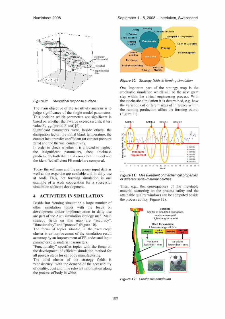
The virtual sensitivity analysis for the determination of significant parameters was conducted using the Response surface methodology (RSM). The RSM is based on mathematical and statistical techniques in order to create optimized empirical models by e.g. multiple regressions. These models are used to describe the relationship between input parameters and one or more responses. Input variables in this analysis were eleven parameters that describe the material behavior, the contact conditions and the production process. The required design of experiments (DoE) that includes the level of variation of the independent input variables and the number of simulation runs was performed with the modul LS-OPT, a commercial statistical program [5]. The forming simulations were accomplished with the general purpose FE-program LS-Dyna (Version 971). The empirical model, based on the experimental data was created and optimised with a commercial statistical program. A well known method to fit empirical models is the method of least square fit which is typically used to estimate the regression coefficients in a multiple linear regression model. In this method, the coefficients of the model have to be adapted until the residual sum of squares is minimized. Residuals are the difference between an observed value of a response variable (simulation result) and the corresponding value predicted by the model (Figure 9).

555


residual

experimentaldata

estimatorof the model

Figure 9: Theoretical response surface

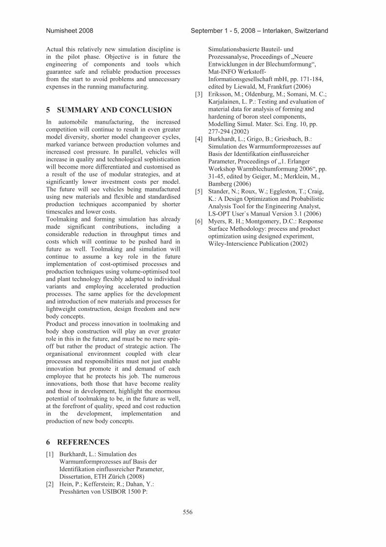
The main objective of the sensitivity analysis is to judge significance of the single model parameters. This decision which parameters are significant is based on whether the F-value exceeds a critical test value Fα,1,n-p (partial F-test) [6]. Significant parameters were, beside others, the dissipation factor, the initial blank temperature, the contact heat transfer coefficient (at contact pressure zero) and the thermal conductivity. In order to check whether it is allowed to neglect the insignificant parameters, sheet thickness predicted by both the initial complex FE model and the identified efficient FE model are compared. Today the software and the necessary input data as well as the expertise are available and in daily use at Audi. Thus, hot forming simulation is one example of a Audi cooperation for a successful simulation software development. 4 ACTIVITIES IN SIMULATION Beside hot forming simulation a large number of other simulation topics with the focus on development and/or implementation in daily use are part of the Audi simulation strategy map. Main strategy fields on this map are “accuracy”, “functionality” and “process” (Figure 10). The focus of topics situated in the “accuracy” cluster is an improvement of the simulation result accuracy by an improvement of FE-codes and input parameters e.g. material parameters. “Functionality” specifies topics with the focus on the development of efficient simulation method for all process steps for car body manufacturing. The third cluster of the strategy fields is “consistency” with the demand of the accessibility of quality, cost and time relevant information along the process of body in white.

Figure 10: Strategy fields in forming simulation

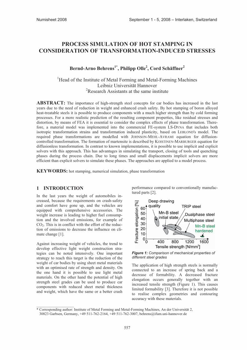
One important part of the strategy map is the stochastic simulation which will be the next great step within the virtual engineering process. With the stochastic simulation it is determined, e.g. how the variations of different sizes of influence within the running production affect the forming output (Figure 11).

30

35

40

45

50

55

0 5 10 15 20 25 30 35 40 45 50 55 60 65 70 75 80 85 90 95lfde. Nr.

Deh

ngre

nze

A 80 [

%]

Kaltband 1Kaltband 2Kaltband 3Kaltband 4Kaltband 5Kaltband 6Kaltband 7Kaltband 9Kaltband 8Kaltband 10

minimum-requirement

Bre

akin

g st

rain

A80

[%]

batch 1 batch 4 batch 6 batch 8

30

35

40

45

50

55

0 5 10 15 20 25 30 35 40 45 50 55 60 65 70 75 80 85 90 95lfde. Nr.

Deh

ngre

nze

A 80 [

%]

Kaltband 1Kaltband 2Kaltband 3Kaltband 4Kaltband 5Kaltband 6Kaltband 7Kaltband 9Kaltband 8Kaltband 10

minimum-requirement

Bre

akin

g st

rain

A80

[%]

batch 1 batch 4 batch 6 batch 8

Figure 11: Measurement of mechanical properties of different serial-material batches

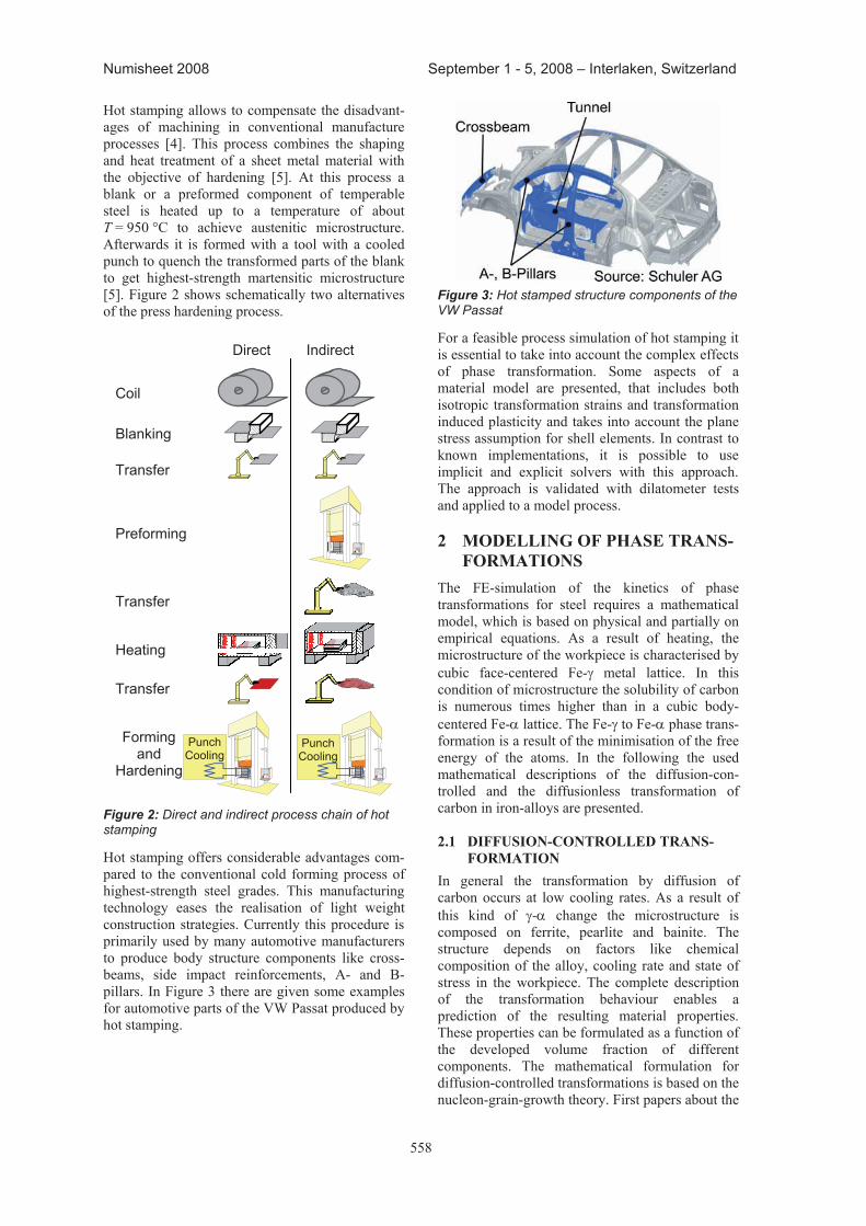
Thus, e.g., the consequences of the inevitable material scattering on the process safety and the attainable quality windows can be computed beside the process ability (Figure 12).

Example: Scatter of simulated springback,

reinforcement-part, high-strength-material

Used for example: tolerance-range ±0,5mm

variations less than 1 mm

variations larger than 1 mm

Figure 12: Stochastic simulation

556


Actual this relatively new simulation discipline is in the pilot phase. Objective is in future the engineering of components and tools which guarantee safe and reliable production processes from the start to avoid problems and unnecessary expenses in the running manufacturing. 5 SUMMARY AND CONCLUSION In automobile manufacturing, the increased competition will continue to result in even greater model diversity, shorter model changeover cycles, marked variance between production volumes and increased cost pressure. In parallel, vehicles will increase in quality and technological sophistication will become more differentiated and customised as a result of the use of modular strategies, and at significantly lower investment costs per model. The future will see vehicles being manufactured using new materials and flexible and standardised production techniques accompanied by shorter timescales and lower costs. Toolmaking and forming simulation has already made significant contributions, including a considerable reduction in throughput times and costs which will continue to be pushed hard in future as well. Toolmaking and simulation will continue to assume a key role in the future implementation of cost-optimised processes and production techniques using volume-optimised tool and plant technology flexibly adapted to individual variants and employing accelerated production processes. The same applies for the development and introduction of new materials and processes for lightweight construction, design freedom and new body concepts. Product and process innovation in toolmaking and body shop construction will play an ever greater role in this in the future, and must be no mere spin-off but rather the product of strategic action. The organisational environment coupled with clear processes and responsibilities must not just enable innovation but promote it and demand of each employee that he protects his job. The numerous innovations, both those that have become reality and those in development, highlight the enormous potential of toolmaking to be, in the future as well, at the forefront of quality, speed and cost reduction in the development, implementation and production of new body concepts.

6 REFERENCES [1] Burkhardt, L.: Simulation des

Warmumformprozesses auf Basis der Identifikation einflussreicher Parameter, Dissertation, ETH Zürich (2008)

[2] Hein, P.; Kefferstein; R.; Dahan, Y.: Presshärten von USIBOR 1500 P:

Simulationsbasierte Bauteil- und Prozessanalyse, Proceedings of „Neuere Entwicklungen in der Blechumformung“, Mat-INFO Werkstoff-Informationsgesellschaft mbH, pp. 171-184, edited by Liewald, M, Frankfurt (2006)

[3] Eriksson, M.; Oldenburg, M.; Somani, M. C.; Karjalainen, L. P.: Testing and evaluation of material data for analysis of forming and hardening of boron steel components, Modelling Simul. Mater. Sci. Eng. 10, pp. 277-294 (2002)

[4] Burkhardt, L.; Grigo, B.; Griesbach, B.: Simulation des Warmumformprozesses auf Basis der Identifikation einflussreicher Parameter, Proceedings of „1. Erlanger Workshop Warmblechumformung 2006“, pp. 31-45, edited by Geiger, M.; Merklein, M., Bamberg (2006)

[5] Stander, N.; Roux, W.; Eggleston, T.; Craig, K.: A Design Optimization and Probabilistic Analysis Tool for the Engineering Analyst, LS-OPT User`s Manual Version 3.1 (2006)

[6] Myers, R. H.; Montgomery, D.C.: Response Surface Methodology: process and product optimization using designed experiment, Wiley-Interscience Publication (2002)

557


prOCeSS SIMULatION OF hOt StaMpING IN CONSIDeratION OF traNSFOrMatION-INDUCeD StreSSeS

Bernd-arno Behrens1*, philipp Olle2, Cord Schäffner2

1Head of the Institute of Metal Forming and Metal-Forming Machines

Leibniz Universität Hannover 2Research Assistants at the same institute

aBStraCt: The importance of high-strength steel concepts for car bodies has increased in the last years due to the need of reduction in weight and enhanced crash safety. By hot stamping of boron alloyed heat-treatable steels it is possible to produce components with a much higher strength than by cold forming processes. For a more realistic prediction of the resulting component properties, like residual stresses and distortion, by means of FEA it is essential to consider the complex effects of phase transformation. There-fore, a material model was implemented into the commercial FE-system LS-DYNA that includes both isotropic transformation strains and transformation induced plasticity, based on LEBLOND's model. The required phase transformations are modelled with JOHNSON-MEHL-AVRAMI equation for diffusion-controlled transformation. The formation of martensite is described by KOISTINEN-MARBURGER equation for diffusionless transformation. In contrast to known implementations, it is possible to use implicit and explicit solvers with this approach. This has advantages in simulating the transport, closing of tools and quenching phases during the process chain. Due to long times and small displacements implicit solvers are more efficient than explicit solvers to simulate these phases. The approaches are applied to a model process.

KeYWOrDS: hot stamping, numerical simulation, phase transformation 1 INtrODUCtIONIn the last years the weight of automobiles in-creased, because the requirements on crash-safety and comfort have gone up, and the vehicles are equipped with comprehensive accessories. The weight increase is leading to higher fuel consump-tion and the involved emissions, for example of CO2. This is in conflict with the effort of the reduc-tion of emissions to decrease the influence on cli-mate change [1]. Against increasing weight of vehicles, the trend to develop effective light weight construction stra-tegies can be noted intensively. One important strategy to reach this target is the reduction of the weight of car bodies by using sheet metal materials with an optimised rate of strength and density. On the one hand it is possible to use light metal materials. On the other hand the potential of high strength steel grades can be used to produce car components with reduced sheet metal thickness and weight, which have the same or a better crash

performance compared to conventionally manufac-tured parts [2].

Figure 1: Comparison of mechanical properties of different steel grades

The application of high strength steels is normally connected to an increase of spring back and a decrease of formability. A decreased fracture elongation occurs generally together with an increased tensile strength (Figure 1). This causes limited formability [3]. Therefore it is not possible to realise complex geometries and contouring accuracy with these materials.

____________________ * Corresponding author: Institute of Metal Forming and Metal-Forming Machines, An der Universität 2, 30823 Garbsen, Germany, +49 511-762-2164, +49 511-762-3007, [email protected]

558


Hot stamping allows to compensate the disadvant-ages of machining in conventional manufacture processes [4]. This process combines the shaping and heat treatment of a sheet metal material with the objective of hardening [5]. At this process a blank or a preformed component of temperable steel is heated up to a temperature of about T = 950 °C to achieve austenitic microstructure. Afterwards it is formed with a tool with a cooled punch to quench the transformed parts of the blank to get highest-strength martensitic microstructure [5]. Figure 2 shows schematically two alternatives of the press hardening process.

Figure 2: Direct and indirect process chain of hot stamping

Hot stamping offers considerable advantages com-pared to the conventional cold forming process of highest-strength steel grades. This manufacturing technology eases the realisation of light weight construction strategies. Currently this procedure is primarily used by many automotive manufacturers to produce body structure components like cross-beams, side impact reinforcements, A- and B-pillars. In Figure 3 there are given some examples for automotive parts of the VW Passat produced by hot stamping.

Figure 3: Hot stamped structure components of the VW Passat

For a feasible process simulation of hot stamping it is essential to take into account the complex effects of phase transformation. Some aspects of a material model are presented, that includes both isotropic transformation strains and transformation induced plasticity and takes into account the plane stress assumption for shell elements. In contrast to known implementations, it is possible to use implicit and explicit solvers with this approach. The approach is validated with dilatometer tests and applied to a model process.

Indirect

PunchCooling

Blanking

Coil

Transfer

Heating

Transfer

Formingand

Hardening

Direct

Preforming

Transfer

PunchCooling

2 MODeLLING OF phaSe traNS-

FOrMatIONSThe FE-simulation of the kinetics of phase transformations for steel requires a mathematical model, which is based on physical and partially on empirical equations. As a result of heating, the microstructure of the workpiece is characterised by cubic face-centered Fe- metal lattice. In this condition of microstructure the solubility of carbon is numerous times higher than in a cubic body-centered Fe- lattice. The Fe- to Fe- phase trans-formation is a result of the minimisation of the free energy of the atoms. In the following the used mathematical descriptions of the diffusion-con-trolled and the diffusionless transformation of carbon in iron-alloys are presented. 2.1 DIFFUSION-CONtrOLLeD traNS-

FOrMatIONIn general the transformation by diffusion of carbon occurs at low cooling rates. As a result of this kind of - change the microstructure is composed on ferrite, pearlite and bainite. The structure depends on factors like chemical composition of the alloy, cooling rate and state of stress in the workpiece. The complete description of the transformation behaviour enables a prediction of the resulting material properties. These properties can be formulated as a function of the developed volume fraction of different components. The mathematical formulation for diffusion-controlled transformations is based on the nucleon-grain-growth theory. First papers about the

559


kinetics of this kind of diffusion-processes were published by AVRAMI [6]. The law of evolution of a structural constituent can be expressed in the generally accepted equation

n

0k

eq( ) 1tt

t e (1)

where is the volume fraction of the growing phase and t/t0 the scaled time. Moreover eq is the phase fraction in equilibirium. In addition, the theoretical formulation of phase evolution was confirmed by experimental investigations of JOHNSON and MEHL [7]. The factor k considers the velocity of migration of the interface and some time independent values to describe the nucleation. The factor n represents the kind of grain growth. Both parameters can be derived from an isotherm time-temperature-transformation diagram. 2.2 DIFFUSIONLeSS traNSFOrMatION If the cooling rate in a quenching process is above a specific critical cooling rate depending on the material, the Fe- to martensite phase transfor-mation takes place. Martensite is characterized by a high mechanical strength. The martensitic trans-formation also depends on chemical composition, especially the carbon fraction, alloying elements and the stress state in the workpiece. The martensite (diffusionless) transformation re-quires a different mathematical approach, because this transformation occurs very fast and without diffusion of carbon. The kinetics of this phase transformation can be described by the function

Ms

Μ ( ) 1T T

t e (2)

where M is the volume fraction of martensite, TMs is the martensite start temperature, T is the temper-ature and and are coefficients. This function was first formulated by KOISTINEN and MARBUR-GER [8] and enhanced by INOUE and WAMG [9]. HOUGARDY [10] verified this formula for the description of the martensite transformation and approximated the coefficients and with the formulas in Table 1. Table 1: Approximation of values of KOISTINEN andMARBURGER equation, see [10]

parameter approximation 0.36·10 + 0.1·10–2 –4 TMs –

0.34·10–6 TMs2 + 0.32·10–8 TMs

3

– 0.52·10–11 TMs4

2.08 – 0.76·10 –2 TMs + 0.16·10 –4 T

3 MaterIaL MODeL For taking into account the phase transformation during simulation of press hardening a material model was implemented into the commercial FE-system LS-DYNA Version 971. In order to model the thermo-elasto-plastic-metallurgical behaviour the total strain increment

el pl th tr tpd d d +d d dij ij ij ij ij ij (3)

can be described by the sum of the elastic, the plastic, the thermal, the isotropic transformation and the transformation-induced plasiticity (trip) strain increment. The thermal and isotropic strain increments are combined to

nth+tr

n

d 1t t t t

ij ijt t

a Ta T

(4)

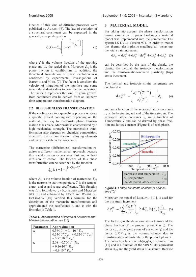
and are a function of the averaged lattice constantsan at the beginning and end of the time step t. The averaged lattice constants an are a function of Temperature T and can be derived by phase frac-tion and lattice constant (Figure 4) of each phase.

Figure 4: Lattice constants of different phases, see [10]

Moreover the model of LEBLOND, [11], is used for the trip strain increment

4tp

=1 y,

dd 3 h d ln ijij k k

k k

sVV

. (5)

The factor sij is the deviatoric stress tensor and the phase fraction of the product phase k is k. The factor y, is the yield stress of austenite ( and the factor (dV/V) k is the volume change due to transformation of austenite in the product phase k . The correction function h=h( vM/ y, ) is taken from [11] and is a function of the VON MISES equivalent stress vM and the yield stress of austenite. Because

TMs 2

– 0.9·10–8 TTMs 3

560


more than one product phase can be generated in one time step it is sumed up over all product phase k. For implicit solution methods the consistent tangent stiffness matrix

2 2 4 2 2

B 1 213

K K KD I I I I I s s (6)

which is derived by simplifying the approach of GEIJSELAERS, [12], is used with the shear modulus G and the bulk modulus KB. The deviatoric stress tensor is denoted by s and the numbers over the unity tensors I represent the tensor's order. More-over the two coefficients K

B

1, K2 are defined as y

1 pl tpy

23 d d

GK

G (7)

and as

y pl tpy pl

2y

ypl

d3 d d

dd

1d

GK (8)

The equivalent plastic strain increment is d pl and the the factor d tp is defined by

4tp

=1

dd 2 h d lnk k

kk

VV

(9)

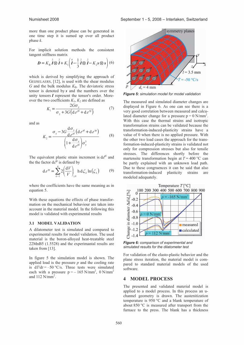
where the coefficients have the same meaning as in equation 5. With these equations the effects of phase transfor-mation on the mechanical behaviour are taken into account in the material model. In the following this model is validated with experimental results 3.1 MODeL VaLIDatION A dilatometer test is simulated and compared to experimental results for model validation. The used material is the boron-alloyed heat-treatable steel 22MnB5 (1.5528) and the experimantal results are taken from [13]. In figure 5 the simulation model is shown. The applied load is the pressure p and the cooling rate is dT/dt = –50 °C/s. Three tests were simulated each with a pressure p = – 165 N/mm , 0 N/mm and 112 N/mm .

2 2

2

Figure 5: simulation model for model validation

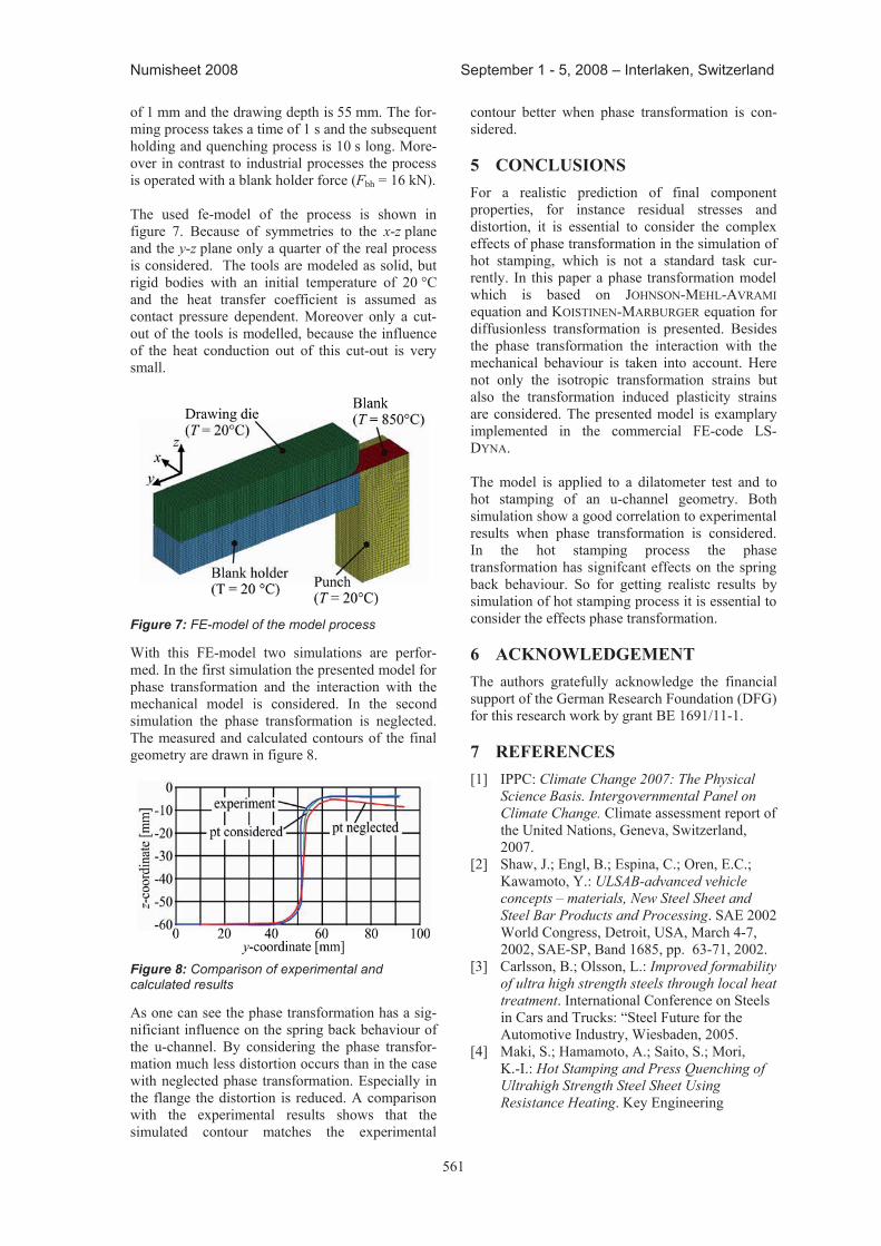
The measured and simulated diameter changes are displayed in Figure 6. As one can see there is a very good correlation between measured and calcu-lated diameter change for a pressure p = 0 N/mm2. With this case the thermal strains and isotropic transformation strains can be validated because the transformation-induced-plasticity strains have a value of 0 when there is no applied pressure. With the other two load cases the approach for the trans-formation-induced-plasticity strains is validated not only for compression stresses but also for tensile stresses. The differences shortly before the martensite transformation begin at T = 400 °C can be partly explained with an unknown load path. Due to these congruences it can be said that also transformation-induced plasticity strains are modeled adequately.

Figure 6: comparison of experimental and simulated results for the dilatometer test

For validation of the elasto-plastic behavior and the plane stress iteration, the material model is com-pared to standard material models of the used software. 4 MODeL prOCeSS The presented and validated material model is applied to a model process. In this process an u-channel geometry is drawn. The austenitization temperature is 950 °C and a blank temperature of about 850 °C is measured after transport from the furnace to the press. The blank has a thickness

561


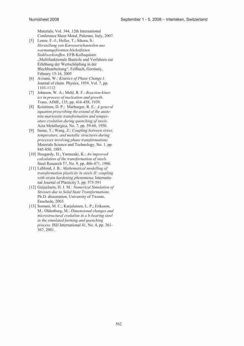
of 1 mm and the drawing depth is 55 mm. The for-ming process takes a time of 1 s and the subsequent holding and quenching process is 10 s long. More-over in contrast to industrial processes the process is operated with a blank holder force (Fbh = 16 kN). The used fe-model of the process is shown in figure 7. Because of symmetries to the x-z plane and the y-z plane only a quarter of the real process is considered. The tools are modeled as solid, but rigid bodies with an initial temperature of 20 °C and the heat transfer coefficient is assumed as contact pressure dependent. Moreover only a cut-out of the tools is modelled, because the influence of the heat conduction out of this cut-out is very small.

Figure 7: FE-model of the model process

With this FE-model two simulations are perfor-med. In the first simulation the presented model for phase transformation and the interaction with the mechanical model is considered. In the second simulation the phase transformation is neglected. The measured and calculated contours of the final geometry are drawn in figure 8.

Figure 8: Comparison of experimental and calculated results

As one can see the phase transformation has a sig-nificiant influence on the spring back behaviour of the u-channel. By considering the phase transfor-mation much less distortion occurs than in the case with neglected phase transformation. Especially in the flange the distortion is reduced. A comparison with the experimental results shows that the simulated contour matches the experimental

contour better when phase transformation is con-sidered. 5 CONCLUSIONS For a realistic prediction of final component properties, for instance residual stresses and distortion, it is essential to consider the complex effects of phase transformation in the simulation of hot stamping, which is not a standard task cur-rently. In this paper a phase transformation model which is based on JOHNSON-MEHL-AVRAMI equation and KOISTINEN-MARBURGER equation for diffusionless transformation is presented. Besides the phase transformation the interaction with the mechanical behaviour is taken into account. Here not only the isotropic transformation strains but also the transformation induced plasticity strains are considered. The presented model is examplary implemented in the commercial FE-code LS-DYNA. The model is applied to a dilatometer test and to hot stamping of an u-channel geometry. Both simulation show a good correlation to experimental results when phase transformation is considered. In the hot stamping process the phase transformation has signifcant effects on the spring back behaviour. So for getting realistc results by simulation of hot stamping process it is essential to consider the effects phase transformation. 6 aCKNOWLeDGeMeNt The authors gratefully acknowledge the financial support of the German Research Foundation (DFG) for this research work by grant BE 1691/11-1. 7 reFereNCeS [1] IPPC: Climate Change 2007: The Physical

Science Basis. Intergovernmental Panel on Climate Change. Climate assessment report of the United Nations, Geneva, Switzerland, 2007.

[2] Shaw, J.; Engl, B.; Espina, C.; Oren, E.C.; Kawamoto, Y.: ULSAB-advanced vehicle concepts – materials, New Steel Sheet and Steel Bar Products and Processing. SAE 2002 World Congress, Detroit, USA, March 4-7, 2002, SAE-SP, Band 1685, pp. 63-71, 2002.

[3] Carlsson, B.; Olsson, L.: Improved formability of ultra high strength steels through local heat treatment. International Conference on Steels in Cars and Trucks: “Steel Future for the Automotive Industry, Wiesbaden, 2005.

[4] Maki, S.; Hamamoto, A.; Saito, S.; Mori, K.-I.: Hot Stamping and Press Quenching of Ultrahigh Strength Steel Sheet Using Resistance Heating. Key Engineering

562


Materials, Vol. 344, 12th International Conference Sheet Metal, Palermo, Italy, 2007.

[5] Lenze, F.-J.; Heller, T.; Sikora, S.: Herstellung von Karosseriebauteilen aus warmumgeformten höchstfesten Stahlwerkstoffen. EFB-Kolloquium: „Multifunktionale Bauteile und Verfahren zur Erhöhung der Wertschöpfung in der Blechbearbeitung“, Fellbach, Germany, Febuary 15-16, 2005

[6] Avrami, W.: Kinetics of Phase Change I. Journal of chem. Physics, 1939, Vol. 7, pp. 1103-1112

[7] Johnson, W. A.; Mehl, R. F.: Reaction kinet-ics in process of nucleation and growth. Trans. AIME, 135, pp. 416-458, 1939.

[8] Koistinen, D. P.; Marburger, R. E.: A general equation prescribing the extend of the auste-nite-martensite transformation and temper-ature evolution during quenching of steels. Acta Metallurgica, No. 7, pp. 59-60, 1950.

[9] Inoue, T.; Wang, Z.: Coupling between stress, temperature, and metallic structures during processes involving phase transformations. Materials Science and Technology, No. 1, pp. 845-850, 1985.

[10] Hougardy, H.; Yamazaki, K.: An improved calculation of the transformation of steels. Steel Research 57, No. 9, pp. 466-471, 1986.

[11] Leblond, J. B.: Mathematical modelling of transformation plasticity in steels II: coupling with strain hardening phenomena. Internatio-nal Journal of Plasticity 5, pp. 573-591

[12] Geijselaers, H. J. M.: Numerical Simulation of Stresses due to Solid State Transformations. Ph.D. dissertation, University of Twente, Enschede, 2003.

[13] Somani, M. C.; Karjalainen, L. P.; Eriksson, M.; Oldenburg, M.: Dimensional changes and microstructural evolution in a b-bearing steel in the simulated forming and quenching process. ISIJ International 41, No. 4, pp. 361-367, 2001.

563


____________________ * Corresponding author: Ingolstädter Str. 102, D-85276 Pfaffenhofen, [email protected]

DeSIGN OF hOtFOrMING prOCeSSeS BaSeD ON SeNSItIVItY aNaLYSIS OF prOCeSS paraMeterS

M. Kerausch1*, t. Schönbach1

1AutoForm Engineering GmbH, Pfaffenhofen, Germany

aBStraCt: The hot-stamping or press hardening technology defined as the combination of hotforming and quenching of highstrengh steel has entered the world wide automotive engineering sector in recent years. Mainly this trend results from the increased requirements concerning passive passenger protection and from the lightweight design efforts. Both requirements challenge new solutions from automotive and supplier industry. Compared to the conventional drawing of high strength steels hot-stamping has two major benefits. Firstly due to the elevated temperature during forming the strain limit is significantly improved while the tool force is on the level of mild steels. Therefore geometrically complex parts can be realised. When the forming process is completed the part rapidly cools down in the closed die. Due to the quenching the strength of the part is increased up to 1500 MPa while the influence of springback is minimized, which is the second major benefit of the press hardening process. The challenge for process design is the complexity and interaction of mechanical and thermal process influences. Therefore the investigations in this paper focus on an effective process layout which is based and conducted with AutoForm-HotForming. The principal sensitivity of typical hot-forming process parameters like the clearance of the blank holder or the initial resting time of the blank on the punch is investigated. By analyzing the different process influences and interactions of the parameters a general approach for the process analysis and process design is derived.

KeYWOrDS: hotforming, process design, sensitivity analysis

1 INtrODUCtION AutoForm provides a complete package of software modules for die shop and sheet metal forming industries. Main goals are to improve the reliability of the planning and layout phase, to reduce the tool testing cycles and therewith to shorten the whole development and tryout time. This objective counts for all upcoming AutoForm software like the HotForming-module which will be presented in this paper. The hot-stamping or press hardening technology defined as the combination of hotforming and quenching of highstrengh steel has entered the world wide automotive engineering sector in recent years [1]. Compared to conventional deep drawing the strain limit is significantly improved due to the elevated temperature during forming while the tool force is on the level of mild steels [2]. Therefore geometrically complex parts can be realised. When the forming process is completed the part rapidly cools down in the closed die. Due to the quenching the strength of the part is increased up to 1500 MPa while the influence of springback is minimized. The challenge for process design is the complexity and interaction of mechanical and thermal process influences.

How to deal with the challenging task to understand the hotforming process and derive a sophisticated strategy for process layout is the subject of this paper and therefore the approach is based on previous investigations conducted by AUDI AG in [3, 4]. Therefore the background for modeling hot-stamping processes with AutoForm-Hotform is presented. Subsequent typical input and process parameters are investigated in sensitivity analysis using AutoForm-Sigma in combination with the HotForming-module. As a benefit the investigation will lead to an increased process understanding, which will support an effective process layout for hot-forming.

2 prOCeSS SIMULatION Compared to conventional deep drawing an extended material description for hot-stamping is necessary due to the thermal influence. The hardening behaviour of boron alloyed steels like 22MnB5, which is mainly used in the automotive industry, is dependent on the temperature. Characteristic for the hot-stamping process is an initial blank temperature of about 850 °C. As the blank is positioned in the draw die contact is established with the cold tool surface, where a

564


temperature of approximately 100 °C can be assumed. In areas, where the blank has no tool contact, the temperature loss takes place because of thermal radiation. These two cases are modelled with a heat transfer coefficient to describe the heat flow either from the blank to the cooler ambient hambient or from the blank into the tool htool. As investigations in [5, 6] have shown, htool is not a constant but dependent on the contact pressure. The dependency is taken into account using htool as a function of contact pressure htool(p) as input data. Because contact surface and contact pressure continuously change during forming, the energy loss of the blank is calculated for every time increment. As mentioned above the temperature change during the forming process significantly influences the local material properties. In general with rising temperature the yield stress decreases and the strain limit increases [7]. To take this into account it is possible to import several flow curves, which are measured for different temperatures, as additional input data for the simulation model. As a second extension to the conventional material description the strain rate has to be considered. In several scientific investigations the strain rate dependency of the steel 22MnB5 is characterized [7, 8, 9]. Typically the strain rates are in the range of 0.1 to 10 1/s during the hot-stamping process. The local strain rate is strongly dependent on the tool velocity and the part geometry. In general the work hardening increases with higher strain rates whereas the forming limit is reduced. This information is, similar to the temperature dependency, modeled in the AutoForm-HotForming material input. Finally the material properties are described as a function of

( )Tk f ,,ϕϕ with a matrix data set of flow curves measured for defined temperatures and strain rates.A complete description of the functionality of the AutoForm-HotForming module is given in [10].

3 DeSIGN aNaLYSIS Using the described procedure concerning the heat transfer and the material property data, it is possible to model and simulate the drawing process for hot-stamping. Furthermore the additional application of AutoForm-Sigma is used to investigate the sensitivity of typical hot-forming parameters by statistical approach. With design analysis the influences of the input and process variables shown in Table 1 are determined. As base process for the stochastic investigations the benchmark ‘BM03 continuous press hardening’ for b-pillar which is proposed by AUDI AG is taken as reference. For this nominal process the effect on the drawing result caused by a change of either input or process parameters is characterized. For this purpose the parameters given in Table 1 are

not assumed as constant like in a conventional simulation but used as design variable with a uniform distribution between the minimum and maximum value. The criterions to set the particular range of the design variables have been on the one hand the uncertainty in determination of

• the heat transfer coefficient htool, • the tool temperature Ttool during forming, • the anisotropy as dependent combination

of r0, r45, r90and • the coefficient of friction µ

and on the other hand the technological and process-related possible range in which

• the blank geometry Geoblank, • the distance of the blankholder Disbh, • the tool velocity TVF and • the initial blank position Posblank in x- and

y-direction can be varied.

Table 1: Design variables

Name Unit Min BM03 Max

Inpu

t

htool W/m2K 3500 4500 5000Ttool °C 25 75 125

r0, 45, 90 - 0.7 1.0 1.0 µ - 0.35 0.40 0.45

proc

ess Geoblank - 0 0.5 1

Disbh mm 0.1 0.4 3.4 TVF - 0.5 1.0 2.0

Posblank mm -5.0 0 5.0

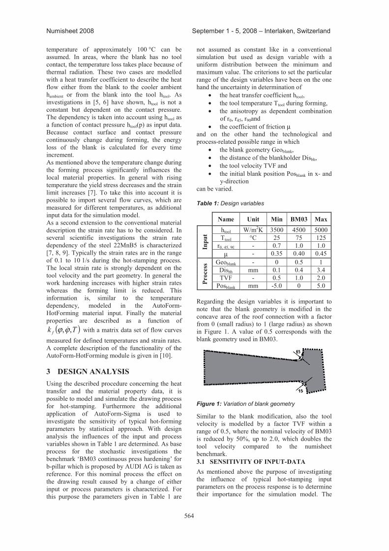
Regarding the design variables it is important to note that the blank geometry is modified in the concave area of the roof connection with a factor from 0 (small radius) to 1 (large radius) as shown in Figure 1. A value of 0.5 corresponds with the blank geometry used in BM03.

Figure 1: Variation of blank geometry

Similar to the blank modification, also the tool velocity is modelled by a factor TVF within a range of 0.5, where the nominal velocity of BM03 is reduced by 50%, up to 2.0, which doubles the tool velocity compared to the numisheet benchmark. 3.1 SeNSItIVItY OF INpUt-Data As mentioned above the purpose of investigating the influence of typical hot-stamping input parameters on the process response is to determine their importance for the simulation model. The

565


main benefit from this is that the process understanding is deepened because of the clear cause-and-effect relation given by the AutoForm-Simga result. Figure 2 shows for example scatter plots for the effect of the heat transfer coefficient htool in comparison to the effect of the tool temperature Ttool on the final blank temperature at the end of the forming process.

Figure 2: Influence of tool temperature vs. heat transfer coefficient on the blank temperature

As the results from the sensitivity analysis in Figure 2 clarify for both input parameters the local temperature loss of the blank during forming strongly depends on the contact situation. In areas where an early punch or die contact is established, like in point A and B, a significant influence can be detected. On the other hand in areas like the door lock connection (point C), where the blank gets contact with the punch at the end of the forming operation, neither htool nor Ttool show a clear effect on the blank temperature. For these three cases the largest temperature loss and scatter range (33°C for htool, 23°C for Ttool) can be observed at the radius in point A. The reason therefore is the high contact pressure of 28±0.7 N/mm2. Because the temperature scatter due to a variation of htool or Ttoolis considerably smaller in most areas of the part, no significant influence on the forming result can be

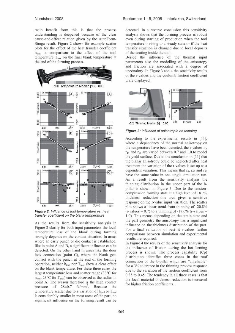
detected. In a reverse conclusion this sensitivity analysis shows that the forming process is robust even during starting of production when the tool temperature is rising to a steady state or if the heat transfer situation is changed due to local deposits of the coating inside the tool. Beside the influence of the thermal input parameters also the modelling of the anisotropy and friction are associated with a degree of uncertainty. In Figure 3 and 4 the sensitivity results of the r-values and the coulomb friction coefficient µ are displayed.

Figure 3: Influence of anisotropie on thinning

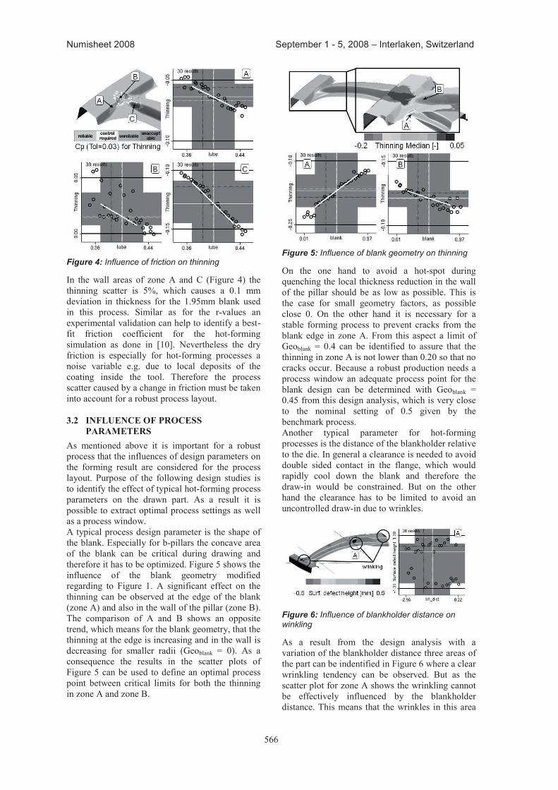
According to the experimental results in [11], where a dependency of the normal anisotropy on the temperature have been detected, the r-values r0, r45 and r90 are varied between 0.7 and 1.0 to model the yield surface. Due to the conclusion in [11] that the planar anisotropy could be neglected after heat treatment the variation of the r-values is set up as a dependent variation. This means that r0, r45 and r90have the same value in one single simulation run. As a result from the sensitivity analysis the thinning distribution in the upper part of the b-pillar is shown in Figure 3. Due to the tension-compression forming state at a high level of 18.7% thickness reduction this area gives a sensitive response on the r-value input variation. The scatter plot shows a linear trend from thinning of -20.8% (r-values = 0.7) to a thinning of -17.6% (r-values = 1.0). This means depending on the strain state and the part geometry the anisotropy has a significant influence on the thickness distribution of the part. For a final validation of best-fit r-values further comparisons between simulation and experimental results are required. In Figure 4 the results of the sensitivity analysis for the influence of friction during the hot-forming process is shown. The process capability (Cp) distribution identifies three zones in the roof connection of the b-pillar which are “unreliable” for a 3% tolerance in the thinning process responsedue to the variation of the friction coefficient from 0.35 to 0.45. The tendency in all three cases is that the local material thickness reduction is increased for higher friction coefficients.

566


Figure 4: Influence of friction on thinning

In the wall areas of zone A and C (Figure 4) the thinning scatter is 5%, which causes a 0.1 mm deviation in thickness for the 1.95mm blank used in this process. Similar as for the r-values an experimental validation can help to identify a best-fit friction coefficient for the hot-forming simulation as done in [10]. Nevertheless the dry friction is especially for hot-forming processes a noise variable e.g. due to local deposits of the coating inside the tool. Therefore the process scatter caused by a change in friction must be taken into account for a robust process layout.

3.2 INFLUeNCe OF prOCeSS paraMeterS

As mentioned above it is important for a robust process that the influences of design parameters on the forming result are considered for the process layout. Purpose of the following design studies is to identify the effect of typical hot-forming process parameters on the drawn part. As a result it is possible to extract optimal process settings as well as a process window. A typical process design parameter is the shape of the blank. Especially for b-pillars the concave area of the blank can be critical during drawing and therefore it has to be optimized. Figure 5 shows the influence of the blank geometry modified regarding to Figure 1. A significant effect on the thinning can be observed at the edge of the blank (zone A) and also in the wall of the pillar (zone B). The comparison of A and B shows an opposite trend, which means for the blank geometry, that the thinning at the edge is increasing and in the wall is decreasing for smaller radii (Geoblank = 0). As a consequence the results in the scatter plots of Figure 5 can be used to define an optimal process point between critical limits for both the thinning in zone A and zone B.

Figure 5: Influence of blank geometry on thinning

On the one hand to avoid a hot-spot during quenching the local thickness reduction in the wall of the pillar should be as low as possible. This isthe case for small geometry factors, as possible close 0. On the other hand it is necessary for a stable forming process to prevent cracks from the blank edge in zone A. From this aspect a limit of Geoblank = 0.4 can be identified to assure that the thinning in zone A is not lower than 0.20 so that no cracks occur. Because a robust production needs a process window an adequate process point for the blank design can be determined with Geoblank = 0.45 from this design analysis, which is very close to the nominal setting of 0.5 given by the benchmark process. Another typical parameter for hot-forming processes is the distance of the blankholder relative to the die. In general a clearance is needed to avoid double sided contact in the flange, which would rapidly cool down the blank and therefore the draw-in would be constrained. But on the other hand the clearance has to be limited to avoid an uncontrolled draw-in due to wrinkles.

Figure 6: Influence of blankholder distance on winkling

As a result from the design analysis with a variation of the blankholder distance three areas of the part can be indentified in Figure 6 where a clear wrinkling tendency can be observed. But as the scatter plot for zone A shows the wrinkling cannot be effectively influenced by the blankholder distance. This means that the wrinkles in this area

567


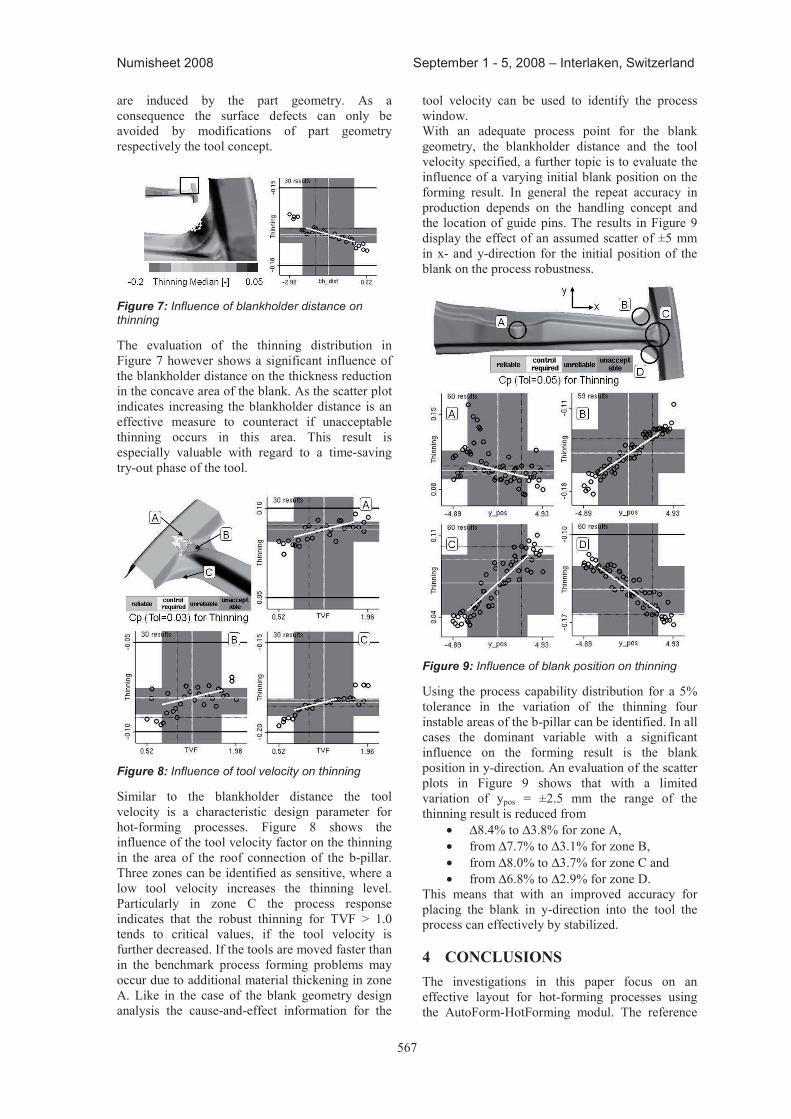
are induced by the part geometry. As a consequence the surface defects can only be avoided by modifications of part geometry respectively the tool concept.

Figure 7: Influence of blankholder distance on thinning

The evaluation of the thinning distribution in Figure 7 however shows a significant influence of the blankholder distance on the thickness reduction in the concave area of the blank. As the scatter plot indicates increasing the blankholder distance is an effective measure to counteract if unacceptable thinning occurs in this area. This result is especially valuable with regard to a time-saving try-out phase of the tool.

Figure 8: Influence of tool velocity on thinning

Similar to the blankholder distance the tool velocity is a characteristic design parameter for hot-forming processes. Figure 8 shows the influence of the tool velocity factor on the thinning in the area of the roof connection of the b-pillar. Three zones can be identified as sensitive, where a low tool velocity increases the thinning level. Particularly in zone C the process response indicates that the robust thinning for TVF > 1.0 tends to critical values, if the tool velocity is further decreased. If the tools are moved faster than in the benchmark process forming problems may occur due to additional material thickening in zone A. Like in the case of the blank geometry design analysis the cause-and-effect information for the

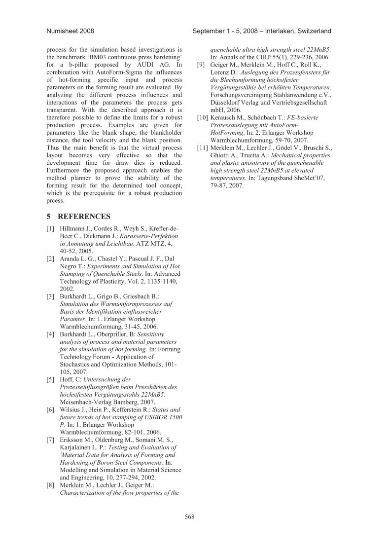
tool velocity can be used to identify the process window. With an adequate process point for the blank geometry, the blankholder distance and the tool velocity specified, a further topic is to evaluate the influence of a varying initial blank position on the forming result. In general the repeat accuracy in production depends on the handling concept and the location of guide pins. The results in Figure 9display the effect of an assumed scatter of ±5 mm in x- and y-direction for the initial position of the blank on the process robustness.

Figure 9: Influence of blank position on thinning

Using the process capability distribution for a 5% tolerance in the variation of the thinning four instable areas of the b-pillar can be identified. In all cases the dominant variable with a significant influence on the forming result is the blank position in y-direction. An evaluation of the scatter plots in Figure 9 shows that with a limited variation of ypos = ±2.5 mm the range of the thinning result is reduced from

• ∆8.4% to ∆3.8% for zone A, • from ∆7.7% to ∆3.1% for zone B, • from ∆8.0% to ∆3.7% for zone C and • from ∆6.8% to ∆2.9% for zone D.

This means that with an improved accuracy for placing the blank in y-direction into the tool the process can effectively by stabilized.

4 CONCLUSIONS The investigations in this paper focus on an effective layout for hot-forming processes using the AutoForm-HotForming modul. The reference

568


process for the simulation based investigations is the benchmark ‘BM03 continuous press hardening’ for a b-pillar proposed by AUDI AG. In combination with AutoForm-Sigma the influences of hot-forming specific input and process parameters on the forming result are evaluated. By analyzing the different process influences and interactions of the parameters the process gets transparent. With the described approach it is therefore possible to define the limits for a robust production process. Examples are given for parameters like the blank shape, the blankholder distance, the tool velocity and the blank position. Thus the main benefit is that the virtual process layout becomes very effective so that the development time for draw dies is reduced. Furthermore the proposed approach enables the method planner to prove the stability of the forming result for the determined tool concept, which is the prerequisite for a robust production prcess.

5 reFereNCeS [1] Hillmann J., Cordes R., Weyh S., Krefter-de-

Beer C., Dickmann J.: Karosserie-Perfektion in Anmutung und Leichtbau. ATZ MTZ, 4, 40-52, 2005.

[2] Aranda L. G., Chastel Y., Pascual J. F., Dal Negro T.: Experiments and Simulation of Hot Stamping of Quenchable Steels. In: Advanced Technology of Plasticity, Vol. 2, 1135-1140, 2002.

[3] Burkhardt L., Grigo B., Griesbach B.: Simulation des Warmumformprozesses auf Basis der Identifikation einflussreicher Paramter. In: 1. Erlanger Workshop Warmblechumformung, 31-45, 2006.

[4] Burkhardt L., Oberpriller, B: Sensitivity analysis of process and material parameters for the simulation of hot forming. In: Forming Technology Forum - Application of Stochastics and Optimization Methods, 101-105, 2007.

[5] Hoff, C: Untersuchung der Prozesseinflussgrößen beim Presshärten des höchstfesten Vergütungsstahls 22MnB5. Meisenbach-Verlag Bamberg, 2007.

[6] Wilsius J., Hein P., Kefferstein R.: Status and future trends of hot stamping of USIBOR 1500 P. In: 1. Erlanger Workshop Warmblechumformung, 82-101, 2006.

[7] Eriksson M., Oldenburg M., Somani M. S., Karjalainen L. P.: Testing and Evaluation of 'Material Data for Analysis of Forming and Hardening of Boron Steel Components. In: Modelling and Simulation in Material Science and Engineering, 10, 277-294, 2002.

[8] Merklein M., Lechler J., Geiger M.: Characterization of the flow properties of the

quenchable ultra high strength steel 22MnB5. In: Annals of the CIRP 55(1), 229-236, 2006

[9] Geiger M., Merklein M., Hoff C., Roll K., Lorenz D.: Auslegung des Prozessfensters für die Blechumformung höchstfester Vergütungsstähle bei erhöhten Temperaturen. Forschungsvereinigung Stahlanwendung e.V., Düsseldorf Verlag und Vertriebsgesellschaft mbH, 2006.

[10] Kerausch M., Schönbach T.: FE-basierte Prozessauslegung mit AutoForm-HotForming. In: 2. Erlanger Workshop Warmblechumformung, 59-70, 2007.

[11] Merklein M., Lechler J., Gödel V., Bruschi S.,Ghiotti A., Truetta A.: Mechanical properties and plastic anisotropy of the quenchenable high strength steel 22MnB5 at elevated temperatures. In: Tagungsband SheMet’07, 79-87, 2007.

569


NUMERICAL SIMULATION OF A THERMO-MECHANICALSHEET METAL FORMING EXPERIMENT

P Akerstrom1, M Oldenburg2∗

1Gestamp HardTech, Lulea, Sweden2Lulea University of Technology, Lulea, Sweden

ABSTRACT: In the design of hot stamped parts, which are subject to both internal and external constraints,it is of great importance to be able to predict the final shape of the component as well as the thickness dis-tribution. It is also important to be able to predict the material state at each point of a component beforeconsideration of the final design of the part itself and the tools. In the present work a model for simulationof the forming and hardening phase in the hot stamping process is evaluated. The model is used in coupledthermo-mechanical simulations and accounts for the effects of micro-structural changes in the material aswell as classical and transformation induced plasticity. The model is evaluated by comparing results from asimulation with a hot stamping experiment. The experimental and the numerically obtained forming force,thickness and shape of the hot stamped component are compared. The evaluation shows that the most impor-tant processes taking place during the thermo-mechanical process are accounted for and that the results fromthe simulation are accurate enough to significantly improve the ability to use simulations as a predictive toolin product development of hot stamped parts.

KEYWORDS: Hot stamping, finite element simulation, microstructure.

1 INTRODUCTION

In this paper, FE-simulation results of the hot stamp-ing process (forming stage) producing a componentis compared to the corresponding experimental re-sults. The main focus is to compare the obtainedfinal shape, hardness and thickness distribution ofthe component. Traditionally when simulating thehot stamping process, the forming stage is often sim-plified by assuming isothermal conditions. In otherwords, no heat transfer between the workpiece andthe environment and the tools are accounted for dur-ing the forming process. Therefore, models describ-ing the decomposition of the initially austenitizedworkpiece into different product phases are not usedin these cases. In the work by Bergman and Olden-burg [1] and Wu et al. [2], the heat transfer betweenthe workpiece and the tool is accounted for, but thecooling rate for all material points are assumed to besufficiently high so the only product phase formedis martensite. In practical hot stamping operationswith the steel grades commonly used, austenite maydecompose into several product phases such as; fer-rite, pearlite, bainite and martensite depending onthe temperature and stress/strain history. The con-tinuous growth of different micro constitutients inthe material affects both the thermal and mechanical

∗Corresponding author: postal address; Lulea University ofTechnology, SE-971 87 Lulea, phone; +46 920 491 752 , fax;+46 920 491 047, email address; [email protected]

properties. In the current work, the rate equationsgiven originally by Kirkaldy and Venugopalan [3]with the modifications proposed by Li et al. [4] areused for the description of the austenite decomposi-tion into product phases. The overall logics for theaustenite decomposition model during the coolingphase follow the algorithm given in Watt et al. [5].The mechanical constitutive model used is an exten-sion of the original model proposed by Leblond et al.[6, 7, 8], Leblond [9] to treat successive transforma-tions, where a detailed description of the model canbe found in Akerstrom et al. [10].In section 2, a description of the experimental toolsand corresponding FE-model is presented. Section 3is used to describe the blank and the correspondingFE-model. In section 4, the experimental equipmentused is described. In section 5, the experimental andsimulated forming results are compared regardingforming force, thickness distribution and final com-ponent shape.

2 TOOLS

In this section a description of the experimental toolsas well as the corresponding FE-model is presented.

2.1 EXPERIMENTAL TOOLS

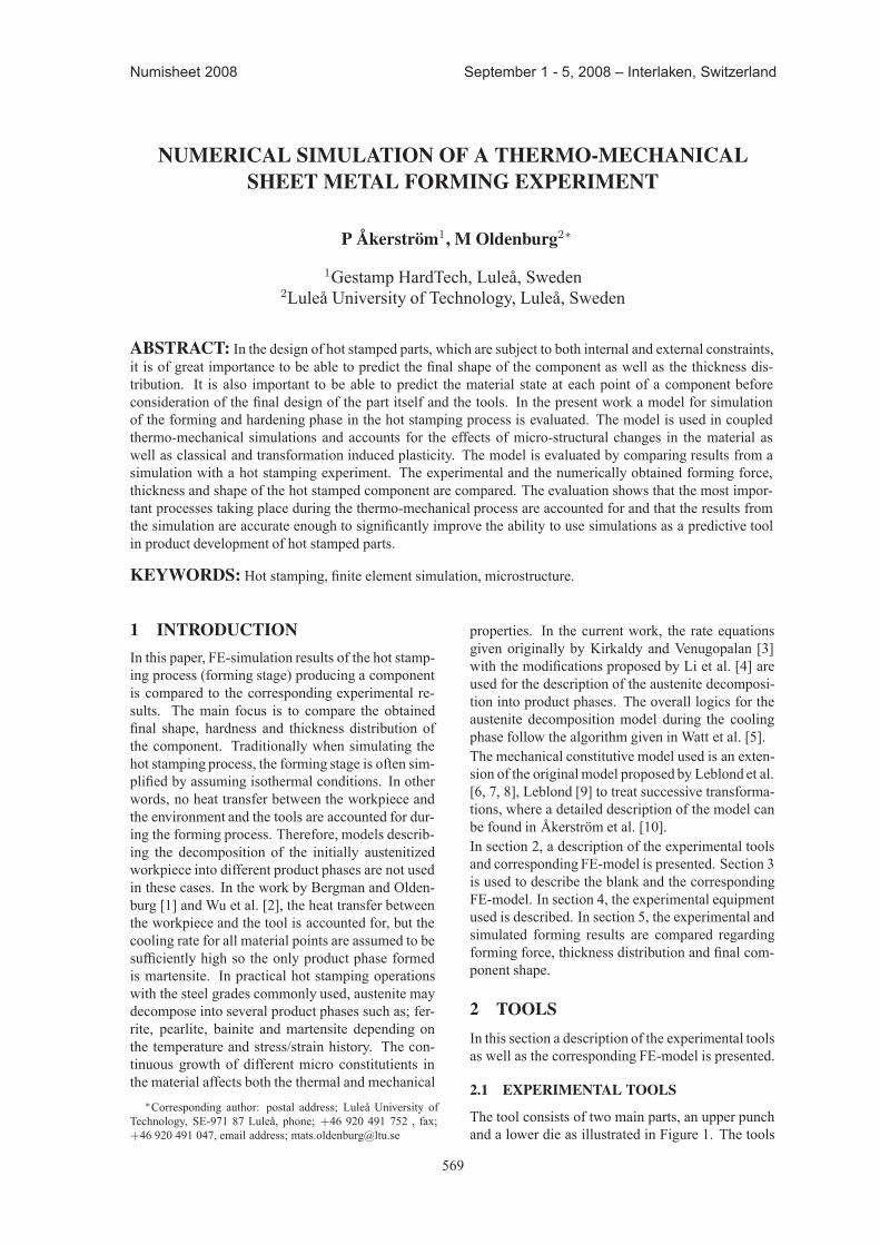
The tool consists of two main parts, an upper punchand a lower die as illustrated in Figure 1. The tools

570


will produce a component with a hat section witha height of 0.052 m (length 0.140 m), that after atransition zone (0.080 m) becomes flat (0.030 m),as can be seen in Figure 1. The final length of thecomponent is ∼0.250 m. Also, as seen in Figure1, some additional components are added to the die.Two additional guiding pins (φ 0.01 m) are used toguide the blank into the correct position in the tool.Further, four small spring supported pins (φ 0.004m) are mounted at the top of the die to prevent thehot blank to come into tool contact during the blankinsertion phase. The material used in the tools isSS2242-02, manufactured by Uddeholm AB [11].The specific heat capacity, cp, and the thermal con-ductivity, k, for the material in the hardened state aregiven in Table 1.

Figure 1: Illustration of tools and the shape of thefinal component.

0.0250.004

0.077

0.004 A

B

0.004

0.050

C

Upper tool

Lower tool

0.0500.10

0.170

0.050

83°

0.040

4×R0.005

4×R0.007

Figure 2: Tool dimensions in the hat-formed section.A, B and C indicate temperature measurement posi-tions. All dimensions are in meters.

2.2 FE-MODEL OF THE TOOLS

The 3D finite element mesh of the tool parts consistsof a total of 57399 eight node brick elements. Dueto symmetry, only half of the tools are modelled.To correctly capture the thermal contact between the

Table 1: Heat capacity and thermal conductivity forSS 2242-02, from [11] and [12].

T[ ◦C] cp[J/kg ◦C] k[W/m ◦C]20 460 25

400 460 29600 460 30

0.168

0.14

00.

180

0.22

0

0.25

3

0.025

0.090

0.015

0.134

0.126

0.125

φ0.0102

φ0.0102

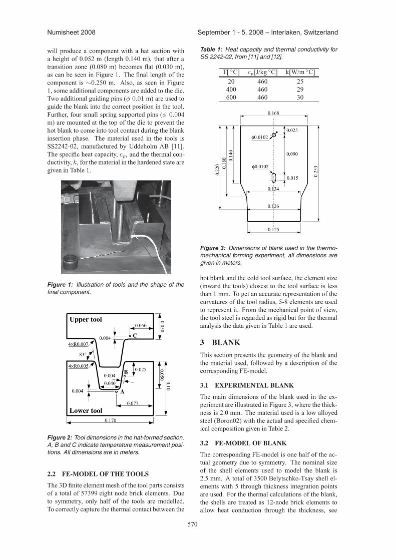
Figure 3: Dimensions of blank used in the thermo-mechanical forming experiment, all dimensions aregiven in meters.

hot blank and the cold tool surface, the element size(inward the tools) closest to the tool surface is lessthan 1 mm. To get an accurate representation of thecurvatures of the tool radius, 5-8 elements are usedto represent it. From the mechanical point of view,the tool steel is regarded as rigid but for the thermalanalysis the data given in Table 1 are used.

3 BLANK

This section presents the geometry of the blank andthe material used, followed by a description of thecorresponding FE-model.

3.1 EXPERIMENTAL BLANK

The main dimensions of the blank used in the ex-periment are illustrated in Figure 3, where the thick-ness is 2.0 mm. The material used is a low alloyedsteel (Boron02) with the actual and specified chem-ical composition given in Table 2.

3.2 FE-MODEL OF BLANK

The corresponding FE-model is one half of the ac-tual geometry due to symmetry. The nominal sizeof the shell elements used to model the blank is2.5 mm. A total of 3500 Belytschko-Tsay shell el-ements with 5 through thickness integration pointsare used. For the thermal calculations of the blank,the shells are treated as 12-node brick elements toallow heat conduction through the thickness, see

571


Table 2: Specified and actual chemical composition for the Boron02 steel (similar to 22MnB5) given in wt%.

C[%] Si[%] Mn[%] Cr[%] P[%] S[%] B[%] Fe[%]Specified 0.2-0.25 0.2-0.35 1.0-1.3 0.15-0.25 <0.025 <0.015 0.0015-0.0050 bal.

Actual 0.248 0.29 1.23 0.24 0.015 0.004 0.0025 bal.

Bergman and Oldenburg [1]. The initial dimensionsof the blank according to Figure 3 are increased 1%to account for the thermal expansion due to heating.To find a good estimate for the initial temperatureto be used in the FE-simulation, a thermocouple iswelded to the blank edge. The flow stress data forthe different phases is extracted from; [13] and [14]for austenite, [15] and [16] for ferrite, [14], [15] and[17] for pearlite, [15] and [18] for bainite, [19] formartensite. Data for thermal conductivity and spe-cific heat for individual phases are extracted fromSjostrom [14]. Values for the latent heat release forthe formation of product phases are; 640 · 106 J/m3

for the austenite to martensite reaction and 590 · 106

J/m3 for all others, which are the values given in[14]. The thermal expansion coefficient used foraustenite is 25 · 10−6 ◦C−1 and for all other con-stituents 11.1 · 10−6 ◦C−1. The compactness differ-ence for the austenite to martensite reaction has beenset to 6.0 · 10−3 and for all others to 4.33 · 10−3

based on the experiments performed in [20]. Forplastic strain, no memory effects are assumed, ex-cept for the bainite transformation, as suggested inPetit-Grostabussiat et al. [18].

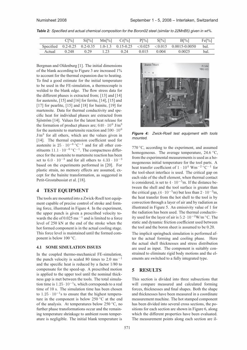
4 TEST EQUIPMENTThe tools are mounted into a Zwick-Roell test equip-ment capable of precise control of stroke and form-ing force, illustrated in Figure 4. In the experiment,the upper punch is given a prescribed velocity to-wards the die of 0.025 ms−1 and is limited to a forcelevel of 250 kN at the end of the stroke when thehot formed component is in the actual cooling stage.This force level is maintained until the formed com-ponent is below 100 ◦C.

4.1 SOME SIMULATION ISSUES

In the coupled thermo-mechanical FE-simulation,the punch velocity is scaled 80 times to 2.0 ms−1

and the specific heat is reduced by a factor 1/80 tocompensate for the speed-up. A prescribed motionis applied to the upper tool until the nominal thick-ness gap is met between the tools. The total simula-tion time is 1.25 ·10−1s, which corresponds to a realtime of 10 s. The simulation time has been chosento 1.25 · 10−1s to ensure that the highest tempera-ture in the component is below 250 ◦C at the endof the analysis. At temperatures below 250 ◦C, nofurther phase transformations occur and the remain-ing temperature shrinkage to ambient room temper-ature is negligible. The initial blank temperature is

Figure 4: Zwick-Roell test equipment with toolsmounted.

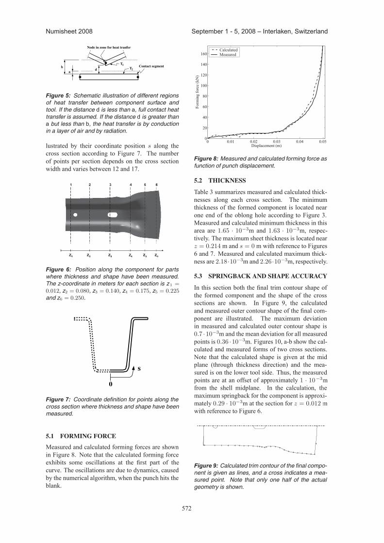
770 ◦C, according to the experiment, and assumedhomogeneous. The average temperature, 24.6 ◦C,from the experimental measurements is used as a ho-mogeneous initial temperature for the tool parts. Aheat transfer coefficient of 1 · 104 Wm−2 ◦C−1 forthe tool-sheet interface is used. The critical gap oneach side of the shell element, when thermal contactis considered, is set to 4 · 10−5m. If the distance be-tween the shell and the tool surface is greater thanthe critical gap, (4 · 10−5m) but less than 2 · 10−3m,the heat transfer from the hot shell to the tool is byconvection through a layer of air and by radiation asillustrated in Figure 5. An emissivity value of 1 forthe radiation has been used. The thermal conductiv-ity used for the layer of air is 5.2 ·10−2W/m ◦C. Thestatic and dynamic friction coefficient used betweenthe tool and the boron sheet is assumed to be 0.20.The implicit springback simulation is performed af-ter the actual forming and cooling phase. Herethe actual shell thicknesses and stress distributionare used as input. The component is suitably con-strained to eliminate rigid body motions and the el-ements are switched to a fully integrated type.

5 RESULTS

This section is divided into three subsections thatwill compare measured and calculated formingforces, thicknesses and final shapes. Both the shapeand thicknesses have been measured in a coordinatemeasurement machine. The hot stamped componenthas been divided into several cross sections, the po-sitions for each section are shown in Figure 6, alongwhich the different properties have been evaluated.The measurement points along each section are il-

572


da

b Contact segmentT1

T2

Node in zone for heat tranfer

Figure 5: Schematic illustration of different regionsof heat transfer between component surface andtool. If the distance d is less than a, full contact heattransfer is assumed. If the distance d is greater thana but less than b, the heat transfer is by conductionin a layer of air and by radiation.

lustrated by their coordinate position s along thecross section according to Figure 7. The numberof points per section depends on the cross sectionwidth and varies between 12 and 17.

Figure 6: Position along the component for partswhere thickness and shape have been measured.The z-coordinate in meters for each section is z1 =0.012, z2 = 0.080, z3 = 0.140, z4 = 0.175, z5 = 0.225and z6 = 0.250.

s

0

Figure 7: Coordinate definition for points along thecross section where thickness and shape have beenmeasured.

5.1 FORMING FORCE

Measured and calculated forming forces are shownin Figure 8. Note that the calculated forming forceexhibits some oscillations at the first part of thecurve. The oscillations are due to dynamics, causedby the numerical algorithm, when the punch hits theblank.

0 0.01 0.02 0.03 0.04 0.050

20

40

60

80

100

120

140

160

Displacement (m)

Form

ing

forc

e (k

N)

CalculatedMeasured

Figure 8: Measured and calculated forming force asfunction of punch displacement.

5.2 THICKNESS

Table 3 summarizes measured and calculated thick-nesses along each cross section. The minimumthickness of the formed component is located nearone end of the oblong hole according to Figure 3.Measured and calculated minimum thickness in thisarea are 1.65 · 10−3m and 1.63 · 10−3m, respec-tively. The maximum sheet thickness is located nearz = 0.214 m and s = 0 m with reference to Figures6 and 7. Measured and calculated maximum thick-ness are 2.18·10−3m and 2.26·10−3m, respectively.

5.3 SPRINGBACK AND SHAPE ACCURACY

In this section both the final trim contour shape ofthe formed component and the shape of the crosssections are shown. In Figure 9, the calculatedand measured outer contour shape of the final com-ponent are illustrated. The maximum deviationin measured and calculated outer contour shape is0.7 ·10−3m and the mean deviation for all measuredpoints is 0.36 ·10−3m. Figures 10, a-b show the cal-culated and measured forms of two cross sections.Note that the calculated shape is given at the midplane (through thickness direction) and the mea-sured is on the lower tool side. Thus, the measuredpoints are at an offset of approximately 1 · 10−3mfrom the shell midplane. In the calculation, themaximum springback for the component is approxi-mately 0.29 · 10−3m at the section for z = 0.012 mwith reference to Figure 6.

Figure 9: Calculated trim contour of the final compo-nent is given as lines, and a cross indicates a mea-sured point. Note that only one half of the actualgeometry is shown.

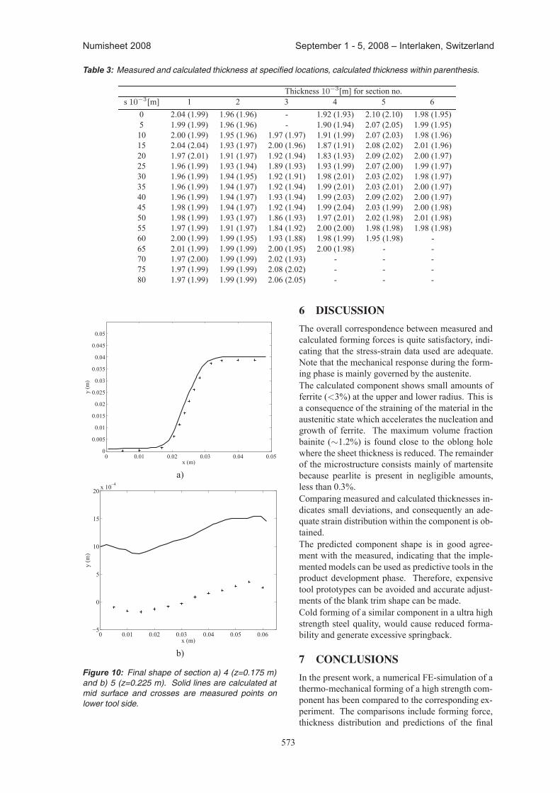
573


Table 3: Measured and calculated thickness at specified locations, calculated thickness within parenthesis.

Thickness 10−3[m] for section no.s 10−3[m] 1 2 3 4 5 6

0 2.04 (1.99) 1.96 (1.96) - 1.92 (1.93) 2.10 (2.10) 1.98 (1.95)5 1.99 (1.99) 1.96 (1.96) - 1.90 (1.94) 2.07 (2.05) 1.99 (1.95)10 2.00 (1.99) 1.95 (1.96) 1.97 (1.97) 1.91 (1.99) 2.07 (2.03) 1.98 (1.96)15 2.04 (2.04) 1.93 (1.97) 2.00 (1.96) 1.87 (1.91) 2.08 (2.02) 2.01 (1.96)20 1.97 (2.01) 1.91 (1.97) 1.92 (1.94) 1.83 (1.93) 2.09 (2.02) 2.00 (1.97)25 1.96 (1.99) 1.93 (1.94) 1.89 (1.93) 1.93 (1.99) 2.07 (2.00) 1.99 (1.97)30 1.96 (1.99) 1.94 (1.95) 1.92 (1.91) 1.98 (2.01) 2.03 (2.02) 1.98 (1.97)35 1.96 (1.99) 1.94 (1.97) 1.92 (1.94) 1.99 (2.01) 2.03 (2.01) 2.00 (1.97)40 1.96 (1.99) 1.94 (1.97) 1.93 (1.94) 1.99 (2.03) 2.09 (2.02) 2.00 (1.97)45 1.98 (1.99) 1.94 (1.97) 1.92 (1.94) 1.99 (2.04) 2.03 (1.99) 2.00 (1.98)50 1.98 (1.99) 1.93 (1.97) 1.86 (1.93) 1.97 (2.01) 2.02 (1.98) 2.01 (1.98)55 1.97 (1.99) 1.91 (1.97) 1.84 (1.92) 2.00 (2.00) 1.98 (1.98) 1.98 (1.98)60 2.00 (1.99) 1.99 (1.95) 1.93 (1.88) 1.98 (1.99) 1.95 (1.98) -65 2.01 (1.99) 1.99 (1.99) 2.00 (1.95) 2.00 (1.98) - -70 1.97 (2.00) 1.99 (1.99) 2.02 (1.93) - - -75 1.97 (1.99) 1.99 (1.99) 2.08 (2.02) - - -80 1.97 (1.99) 1.99 (1.99) 2.06 (2.05) - - -

0 0.01 0.02 0.03 0.04 0.050

0.005

0.01

0.015

0.02

0.025

0.03

0.035

0.04

0.045

0.05

x (m)

y (m

)

a)

0 0.01 0.02 0.03 0.04 0.05 0.06−5

0

5

10

15

20 x 10−4

x (m)

y (m

)

b)

Figure 10: Final shape of section a) 4 (z=0.175 m)and b) 5 (z=0.225 m). Solid lines are calculated atmid surface and crosses are measured points onlower tool side.

6 DISCUSSION

The overall correspondence between measured andcalculated forming forces is quite satisfactory, indi-cating that the stress-strain data used are adequate.Note that the mechanical response during the form-ing phase is mainly governed by the austenite.The calculated component shows small amounts offerrite (<3%) at the upper and lower radius. This isa consequence of the straining of the material in theaustenitic state which accelerates the nucleation andgrowth of ferrite. The maximum volume fractionbainite (∼1.2%) is found close to the oblong holewhere the sheet thickness is reduced. The remainderof the microstructure consists mainly of martensitebecause pearlite is present in negligible amounts,less than 0.3%.Comparing measured and calculated thicknesses in-dicates small deviations, and consequently an ade-quate strain distribution within the component is ob-tained.The predicted component shape is in good agree-ment with the measured, indicating that the imple-mented models can be used as predictive tools in theproduct development phase. Therefore, expensivetool prototypes can be avoided and accurate adjust-ments of the blank trim shape can be made.Cold forming of a similar component in a ultra highstrength steel quality, would cause reduced forma-bility and generate excessive springback.

7 CONCLUSIONS

In the present work, a numerical FE-simulation of athermo-mechanical forming of a high strength com-ponent has been compared to the corresponding ex-periment. The comparisons include forming force,thickness distribution and predictions of the final

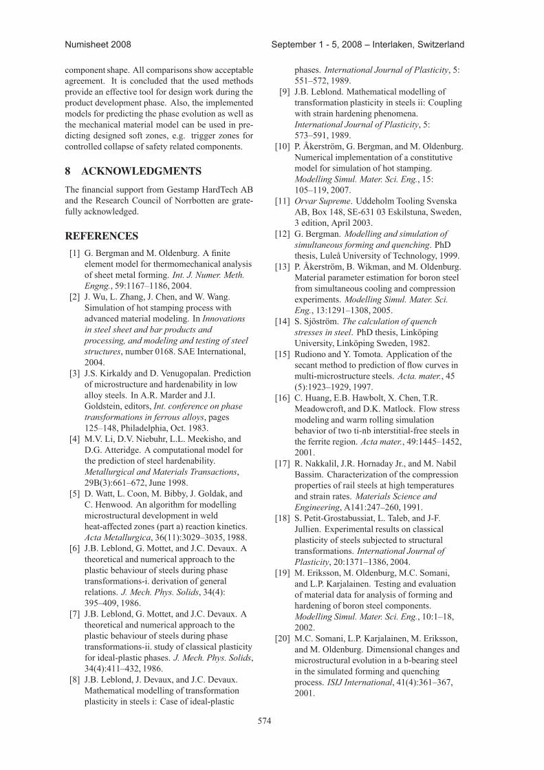
574


component shape. All comparisons show acceptableagreement. It is concluded that the used methodsprovide an effective tool for design work during theproduct development phase. Also, the implementedmodels for predicting the phase evolution as well asthe mechanical material model can be used in pre-dicting designed soft zones, e.g. trigger zones forcontrolled collapse of safety related components.

8 ACKNOWLEDGMENTS

The financial support from Gestamp HardTech ABand the Research Council of Norrbotten are grate-fully acknowledged.

REFERENCES

[1] G. Bergman and M. Oldenburg. A finiteelement model for thermomechanical analysisof sheet metal forming. Int. J. Numer. Meth.Engng., 59:1167–1186, 2004.

[2] J. Wu, L. Zhang, J. Chen, and W. Wang.Simulation of hot stamping process withadvanced material modeling. In Innovationsin steel sheet and bar products andprocessing, and modeling and testing of steelstructures, number 0168. SAE International,2004.

[3] J.S. Kirkaldy and D. Venugopalan. Predictionof microstructure and hardenability in lowalloy steels. In A.R. Marder and J.I.Goldstein, editors, Int. conference on phasetransformations in ferrous alloys, pages125–148, Philadelphia, Oct. 1983.

[4] M.V. Li, D.V. Niebuhr, L.L. Meekisho, andD.G. Atteridge. A computational model forthe prediction of steel hardenability.Metallurgical and Materials Transactions,29B(3):661–672, June 1998.

[5] D. Watt, L. Coon, M. Bibby, J. Goldak, andC. Henwood. An algorithm for modellingmicrostructural development in weldheat-affected zones (part a) reaction kinetics.Acta Metallurgica, 36(11):3029–3035, 1988.

[6] J.B. Leblond, G. Mottet, and J.C. Devaux. Atheoretical and numerical approach to theplastic behaviour of steels during phasetransformations-i. derivation of generalrelations. J. Mech. Phys. Solids, 34(4):395–409, 1986.

[7] J.B. Leblond, G. Mottet, and J.C. Devaux. Atheoretical and numerical approach to theplastic behaviour of steels during phasetransformations-ii. study of classical plasticityfor ideal-plastic phases. J. Mech. Phys. Solids,34(4):411–432, 1986.

[8] J.B. Leblond, J. Devaux, and J.C. Devaux.Mathematical modelling of transformationplasticity in steels i: Case of ideal-plastic

phases. International Journal of Plasticity, 5:551–572, 1989.

[9] J.B. Leblond. Mathematical modelling oftransformation plasticity in steels ii: Couplingwith strain hardening phenomena.International Journal of Plasticity, 5:573–591, 1989.

[10] P. Akerstrom, G. Bergman, and M. Oldenburg.Numerical implementation of a constitutivemodel for simulation of hot stamping.Modelling Simul. Mater. Sci. Eng., 15:105–119, 2007.

[11] Orvar Supreme. Uddeholm Tooling SvenskaAB, Box 148, SE-631 03 Eskilstuna, Sweden,3 edition, April 2003.

[12] G. Bergman. Modelling and simulation ofsimultaneous forming and quenching. PhDthesis, Lulea University of Technology, 1999.

[13] P. Akerstrom, B. Wikman, and M. Oldenburg.Material parameter estimation for boron steelfrom simultaneous cooling and compressionexperiments. Modelling Simul. Mater. Sci.Eng., 13:1291–1308, 2005.

[14] S. Sjostrom. The calculation of quenchstresses in steel. PhD thesis, LinkopingUniversity, Linkoping Sweden, 1982.

[15] Rudiono and Y. Tomota. Application of thesecant method to prediction of flow curves inmulti-microstructure steels. Acta. mater., 45(5):1923–1929, 1997.

[16] C. Huang, E.B. Hawbolt, X. Chen, T.R.Meadowcroft, and D.K. Matlock. Flow stressmodeling and warm rolling simulationbehavior of two ti-nb interstitial-free steels inthe ferrite region. Acta mater., 49:1445–1452,2001.

[17] R. Nakkalil, J.R. Hornaday Jr., and M. NabilBassim. Characterization of the compressionproperties of rail steels at high temperaturesand strain rates. Materials Science andEngineering, A141:247–260, 1991.

[18] S. Petit-Grostabussiat, L. Taleb, and J-F.Jullien. Experimental results on classicalplasticity of steels subjected to structuraltransformations. International Journal ofPlasticity, 20:1371–1386, 2004.

[19] M. Eriksson, M. Oldenburg, M.C. Somani,and L.P. Karjalainen. Testing and evaluationof material data for analysis of forming andhardening of boron steel components.Modelling Simul. Mater. Sci. Eng., 10:1–18,2002.

[20] M.C. Somani, L.P. Karjalainen, M. Eriksson,and M. Oldenburg. Dimensional changes andmicrostructural evolution in a b-bearing steelin the simulated forming and quenchingprocess. ISIJ International, 41(4):361–367,2001.

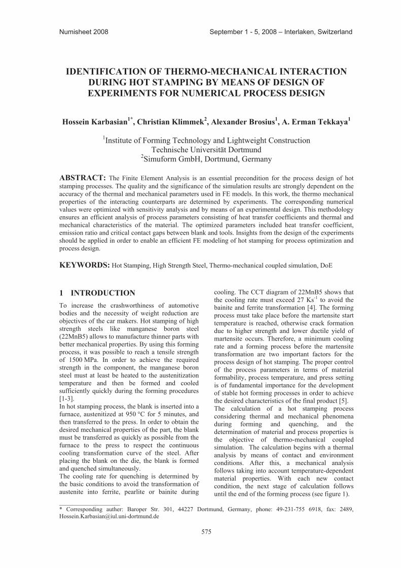
575


____________________* Corresponding auther: Baroper Str. 301, 44227 Dortmund, Germany, phone: 49-231-755 6918, fax: 2489, [email protected]

IDeNtIFICatION OF therMO-MeChaNICaL INteraCtION DUrING hOt StaMpING BY MeaNS OF DeSIGN OF eXperIMeNtS FOr NUMerICaL prOCeSS DeSIGN

hossein Karbasian1*, Christian Klimmek2, alexander Brosius1, a. erman tekkaya1

1Institute of Forming Technology and Lightweight Construction Technische Universität Dortmund

2Simuform GmbH, Dortmund, Germany

aBStraCt: The Finite Element Analysis is an essential precondition for the process design of hot stamping processes. The quality and the significance of the simulation results are strongly dependent on the accuracy of the thermal and mechanical parameters used in FE models. In this work, the thermo mechanical properties of the interacting counterparts are determined by experiments. The corresponding numerical values were optimized with sensitivity analysis and by means of an experimental design. This methodology ensures an efficient analysis of process parameters consisting of heat transfer coefficients and thermal and mechanical characteristics of the material. The optimized parameters included heat transfer coefficient, emission ratio and critical contact gaps between blank and tools. Insights from the design of the experiments should be applied in order to enable an efficient FE modeling of hot stamping for process optimization and process design.

KeYWOrDS: Hot Stamping, High Strength Steel, Thermo-mechanical coupled simulation, DoE

1 INtrODUCtIONTo increase the crashworthiness of automotive bodies and the necessity of weight reduction are objectives of the car makers. Hot stamping of high strength steels like manganese boron steel (22MnB5) allows to manufacture thinner parts with better mechanical properties. By using this forming process, it was possible to reach a tensile strength of 1500 MPa. In order to achieve the required strength in the component, the manganese boron steel must at least be heated to the austenitization temperature and then be formed and cooled sufficiently quickly during the forming procedures [1-3]. In hot stamping process, the blank is inserted into a furnace, austenitized at 950 °C for 5 minutes, and then transferred to the press. In order to obtain the desired mechanical properties of the part, the blank must be transferred as quickly as possible from the furnace to the press to respect the continuous cooling transformation curve of the steel. After placing the blank on the die, the blank is formed and quenched simultaneously. The cooling rate for quenching is determined by the basic conditions to avoid the transformation of austenite into ferrite, pearlite or bainite during

cooling. The CCT diagram of 22MnB5 shows that the cooling rate must exceed 27 Ks-1 to avoid the bainite and ferrite transformation [4]. The forming process must take place before the martensite start temperature is reached, otherwise crack formation due to higher strength and lower ductile yield of martensite occurs. Therefore, a minimum cooling rate and a forming process before the martensite transformation are two important factors for the process design of hot stamping. The proper control of the process parameters in terms of material formability, process temperature, and press setting is of fundamental importance for the development of stable hot forming processes in order to achieve the desired characteristics of the final product [5]. The calculation of a hot stamping process considering thermal and mechanical phenomena during forming and quenching, and the determination of material and process properties is the objective of thermo-mechanical coupled simulation. The calculation begins with a thermal analysis by means of contact and environment conditions. After this, a mechanical analysis follows taking into account temperature-dependent material properties. With each new contact condition, the next stage of calculation follows until the end of the forming process (see figure 1).

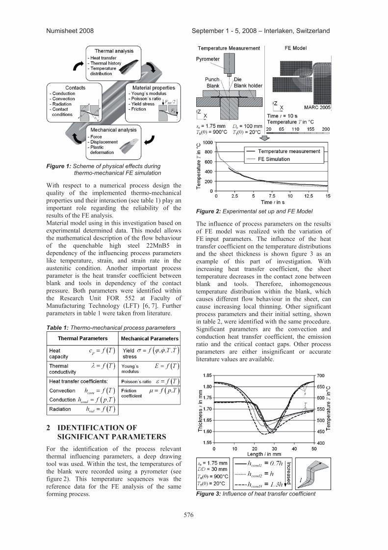
576


Figure 1: Scheme of physical effects during thermo-mechanical FE simulation

With respect to a numerical process design the quality of the implemented thermo-mechanical properties und their interaction (see table 1) play an important role regarding the reliability of the results of the FE analysis. Material model using in this investigation based on experimental determined data. This model allows the mathematical description of the flow behaviour of the quenchable high steel 22MnB5 in dependency of the influencing process parameters like temperature, strain, and strain rate in the austenitic condition. Another important process parameter is the heat transfer coefficient between blank and tools in dependency of the contact pressure. Both parameters were identified within the Research Unit FOR 552 at Faculty of Manufacturing Technology (LFT) [6, 7]. Further parameters in table 1 were taken from literature.

Table 1: Thermo-mechanical process parameters

2 IDeNtIFICatION OF SIGNIFICaNt paraMeterS

For the identification of the process relevant thermal influencing parameters, a deep drawing tool was used. Within the test, the temperatures of the blank were recorded using a pyrometer (see figure 2). This temperature sequences was the reference data for the FE analysis of the same forming process.

Figure 2: Experimental set up and FE Model

The influence of process parameters on the results of FE model was realized with the variation of FE input parameters. The influence of the heat transfer coefficient on the temperature distributions and the sheet thickness is shown figure 3 as an example of this part of investigation. With increasing heat transfer coefficient, the sheet temperature decreases in the contact zone between blank and tools. Therefore, inhomogeneous temperature distribution within the blank, which causes different flow behaviour in the sheet, can cause increasing local thinning. Other significant process parameters and their initial setting, shown in table 2, were identified with the same procedure. Significant parameters are the convection and conduction heat transfer coefficient, the emission ratio and the critical contact gaps. Other process parameters are either insignificant or accurate literature values are available.

Figure 3: Influence of heat transfer coefficient

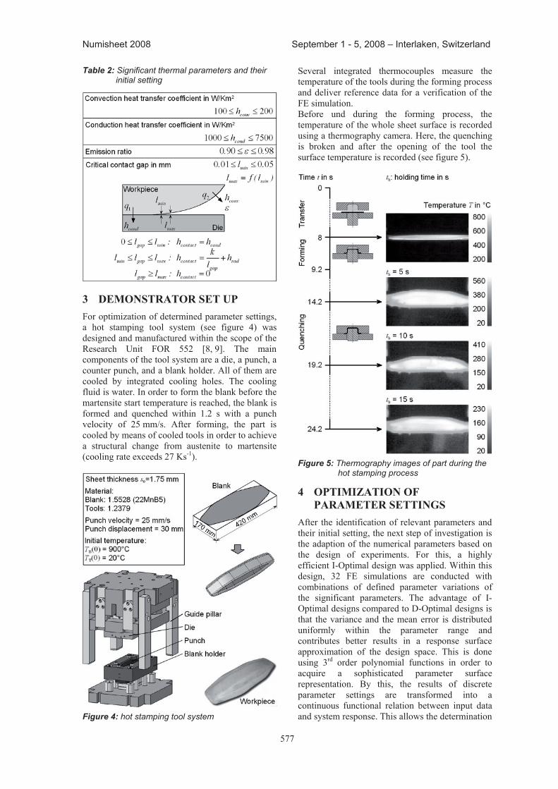
577


Table 2: Significant thermal parameters and their initial setting

3 DeMONStratOr Set Up For optimization of determined parameter settings, a hot stamping tool system (see figure 4) was designed and manufactured within the scope of the Research Unit FOR 552 [8, 9]. The main components of the tool system are a die, a punch, a counter punch, and a blank holder. All of them are cooled by integrated cooling holes. The cooling fluid is water. In order to form the blank before the martensite start temperature is reached, the blank is formed and quenched within 1.2 s with a punch velocity of 25 mm/s. After forming, the part is cooled by means of cooled tools in order to achieve a structural change from austenite to martensite (cooling rate exceeds 27 Ks-1).

Figure 4: hot stamping tool system

Several integrated thermocouples measure the temperature of the tools during the forming process and deliver reference data for a verification of the FE simulation. Before und during the forming process, the temperature of the whole sheet surface is recorded using a thermography camera. Here, the quenching is broken and after the opening of the tool the surface temperature is recorded (see figure 5).

Figure 5: Thermography images of part during the hot stamping process

4 OptIMIZatION OF paraMeter SettINGS

After the identification of relevant parameters and their initial setting, the next step of investigation is the adaption of the numerical parameters based on the design of experiments. For this, a highly efficient I-Optimal design was applied. Within this design, 32 FE simulations are conducted with combinations of defined parameter variations of the significant parameters. The advantage of I-Optimal designs compared to D-Optimal designs is that the variance and the mean error is distributed uniformly within the parameter range and contributes better results in a response surface approximation of the design space. This is done using 3rd order polynomial functions in order to acquire a sophisticated parameter surface representation. By this, the results of discrete parameter settings are transformed into a continuous functional relation between input data and system response. This allows the determination

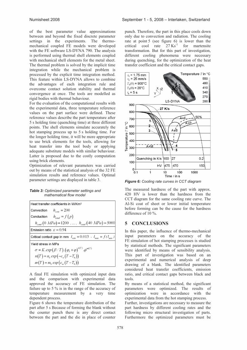
578


of the best parameter value approximations between and beyond the fixed discrete parameter settings in the experiments. The thermo-mechanical coupled FE models were developed with the FE software LS-DYNA 790. The analysis is performed using thermal shell elements coupled with mechanical shell elements for the metal sheet. The thermal problem is solved by the implicit time integration while the mechanical problem is processed by the explicit time integration method. This feature within LS-DYNA allows to combine the advantages of each integration rule and overcome contact solution stability and thermal convergence at once. The tools are modelled as rigid bodies with thermal behaviour. For the evaluation of the computational results with the experimental data, three temperature reference values on the part surface were defined. These reference values describe the part temperature after 5 s holding time (quenching time) at three different points. The shell elements simulate accurately the hot stamping process up to 5 s holding time. For the longer holding time, it will be more appropriate to use brick elements for the tools, allowing for heat transfer into the tool body or applying adequate substitute models with similar behaviour. Latter is proposed due to the costly computation using brick elements. Optimization of relevant parameters was carried out by means of the statistical analysis of the 32 FE simulation results and reference values. Optimal parameter settings are displayed in table 3.

Table 3: Optimized parameter settings and mathematical flow model

A final FE simulation with optimized input data and the comparison with experimental data approved the accuracy of FE simulation. The failure up to 5 % is in the range of the accuracy of temperature measurement by a very time dependent process. Figure 6 shows the temperature distribution of the part after 5 s Because of forming the blank without the counter punch there is any direct contact between the part and the die in place of counter

punch. Therefore, the part in this place cools down only due to convection and radiation. The cooling rate at point 5 (see figure 6) is lower than the critical cool rate 27 Ks-1 for martensite transformation. But for this part of investigation, different cooling phenomena were necessary during quenching, for the optimization of the heat transfer coefficient and the critical contact gaps.

Figure 6: Cooling rate curves in CCT diagram

The measured hardness of the part with approx. 420 HV is lower than the hardness from the CCT diagram for the same cooling rate curve. The Al-Si coat of sheet or lower initial temperature before forming can be the cause for the hardness difference of 10 %.

5 CONCLUSIONS In this paper, the influence of thermo-mechanical input parameters on the accuracy of the FE simulation of hot stamping processes is studied by statistical methods. The significant parameters were identified by means of sensibility analysis. This part of investigation was based on an experimental and numerical analysis of deep drawing of a blank. The identified parameters considered heat transfer coefficients, emission ratio, and critical contact gaps between black and tools. By means of a statistical method, the significant parameters were optimized. The results of optimization were in accordance with the experimental data from the hot stamping process. Further, investigations are necessary to measure the part hardness by different cooling rates and the following micro structural investigation of parts. Furthermore the optimized parameters must be

579


implemented in brick model for the FE simulation of quenching phase allowing for heat transfer in the tools. Therefore, higher accuracies of cooling rate curves for hardness prediction are reachable.

6 aCKNOWLeDGeMeNt The authors thank the German Research Foundation for the financial support within the Research Unit FOR 552.

7 reFereNCeS [1] Sikora, S.; Lenze, F.-J.: Hot-Forming-Process

Important Parameters for the Production of High-Strength BIW Parts. IDDRG 2006, Porto, 295-301

[2] Hein, P.: A Global Approach of the Finite Element Simulation of Hot Stamping.Advanced Materials and Research, Vol. 6-8 (2005), 763-770

[3] Kolleck, R.; Lenze. F.-J.: Warmumformung und Kaltumformung- zwei ergänzende Verfahren für den Karosserieleichtbau.Neuere Entwicklungen in der Blechum-formung, Frankfurt 2004, 345-254

[4] Garcia Aranda, L.; Chastel, Y.; Fernandez Pascual, J.; Dal Negro, T.: Experiments and Simulation of the Hot Stamping of Quenchable Steels. Advanced Technology of Plasticity, Vol. 2, 2002, 1135-1140

[5] Mori, K.; Maki, S.; Tanaka, Y.: Warm and Hot Stamping of Ultra High Tensile Strength Steel Sheets Using Resistance Heating.Annals of the CIRP, 54-1(2005), 209-212

[6] Geiger, M.; Merklein, M.; Lechler, J.; Bach, Fr.-W.; Springer, R.; Kleiner, M.; Homberg, W.; Brosius, A.; Karbasian, H.; Hoffmann, H.; So, H.: Basic Investigations on Hot Sheet Metal Forming of Quenchenable High Strength Steels. 2nd International Conference ob New Forming Technology, 2007, Bremen, 327-336

[7] Merklein, M.; Lechler, J.; Geiger, M.; Kleiner, M.; Karbasian, H., Homberg, W.: Untersuchung der thermo-mechanischen Fließeigenschaften presshärtbarer Stähle. 2nd

International Confrence on Accuracy in Forming Technology ICAFT 2006, in association with 13.th Saxon Confrence on Forming Technology SFU 2006, Chemnitz, 217-234

[8] So, H.; Steinbeiß, H.; Hoffmann, H.: Optimierung von Umformwerkzeugen für die Warmblechumformung. 1. Erlanger Workshop Warmblechumformung (2006), 102-117

[9] Steinbeiß, H.; So, H.; Michelitsch, T.; Hoffmann, H.: Method for optimizing the cooling design of hot stamping tools.Production Engineering - Research and Development, Vol. 1, No. 2 (2007), 149-155

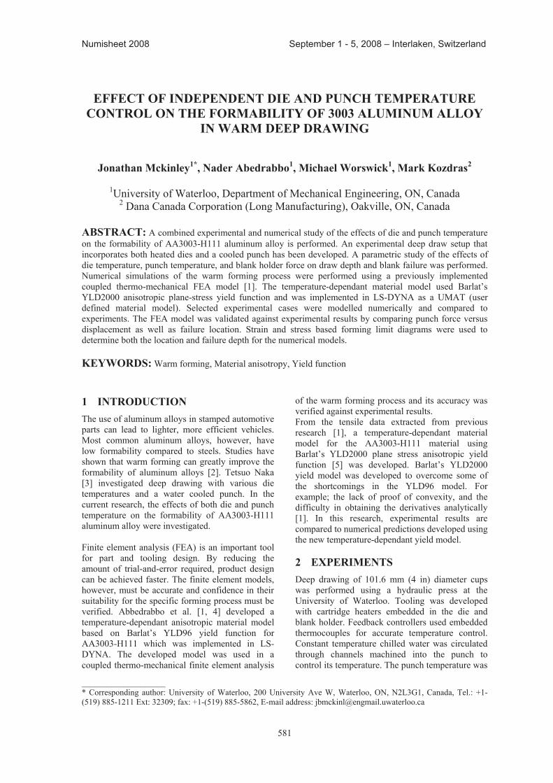
581


____________________ * Corresponding author: University of Waterloo, 200 University Ave W, Waterloo, ON, N2L3G1, Canada, Tel.: +1-(519) 885-1211 Ext: 32309; fax: +1-(519) 885-5862, E-mail address: [email protected]

EFFECT OF INDEPENDENT DIE AND PUNCH TEMPERATURE CONTROL ON THE FORMABILITY OF 3003 ALUMINUM ALLOY

IN WARM DEEP DRAWING

Jonathan Mckinley1*, Nader Abedrabbo1, Michael Worswick1, Mark Kozdras2

1University of Waterloo, Department of Mechanical Engineering, ON, Canada 2 Dana Canada Corporation (Long Manufacturing), Oakville, ON, Canada

ABSTRACT: A combined experimental and numerical study of the effects of die and punch temperature on the formability of AA3003-H111 aluminum alloy is performed. An experimental deep draw setup that incorporates both heated dies and a cooled punch has been developed. A parametric study of the effects of die temperature, punch temperature, and blank holder force on draw depth and blank failure was performed. Numerical simulations of the warm forming process were performed using a previously implemented coupled thermo-mechanical FEA model [1]. The temperature-dependant material model used Barlat’s YLD2000 anisotropic plane-stress yield function and was implemented in LS-DYNA as a UMAT (user defined material model). Selected experimental cases were modelled numerically and compared to experiments. The FEA model was validated against experimental results by comparing punch force versus displacement as well as failure location. Strain and stress based forming limit diagrams were used to determine both the location and failure depth for the numerical models.

KEYWORDS: Warm forming, Material anisotropy, Yield function 1 INTRODUCTION The use of aluminum alloys in stamped automotive parts can lead to lighter, more efficient vehicles. Most common aluminum alloys, however, have low formability compared to steels. Studies have shown that warm forming can greatly improve the formability of aluminum alloys [2]. Tetsuo Naka [3] investigated deep drawing with various die temperatures and a water cooled punch. In the current research, the effects of both die and punch temperature on the formability of AA3003-H111 aluminum alloy were investigated. Finite element analysis (FEA) is an important tool for part and tooling design. By reducing the amount of trial-and-error required, product design can be achieved faster. The finite element models, however, must be accurate and confidence in their suitability for the specific forming process must be verified. Abbedrabbo et al. [1, 4] developed a temperature-dependant anisotropic material model based on Barlat’s YLD96 yield function for AA3003-H111 which was implemented in LS-DYNA. The developed model was used in a coupled thermo-mechanical finite element analysis

of the warm forming process and its accuracy was verified against experimental results. From the tensile data extracted from previous research [1], a temperature-dependant material model for the AA3003-H111 material using Barlat’s YLD2000 plane stress anisotropic yield function [5] was developed. Barlat’s YLD2000 yield model was developed to overcome some of the shortcomings in the YLD96 model. For example; the lack of proof of convexity, and the difficulty in obtaining the derivatives analytically [1]. In this research, experimental results are compared to numerical predictions developed using the new temperature-dependant yield model. 2 EXPERIMENTS Deep drawing of 101.6 mm (4 in) diameter cups was performed using a hydraulic press at the University of Waterloo. Tooling was developed with cartridge heaters embedded in the die and blank holder. Feedback controllers used embedded thermocouples for accurate temperature control. Constant temperature chilled water was circulated through channels machined into the punch to control its temperature. The punch temperature was

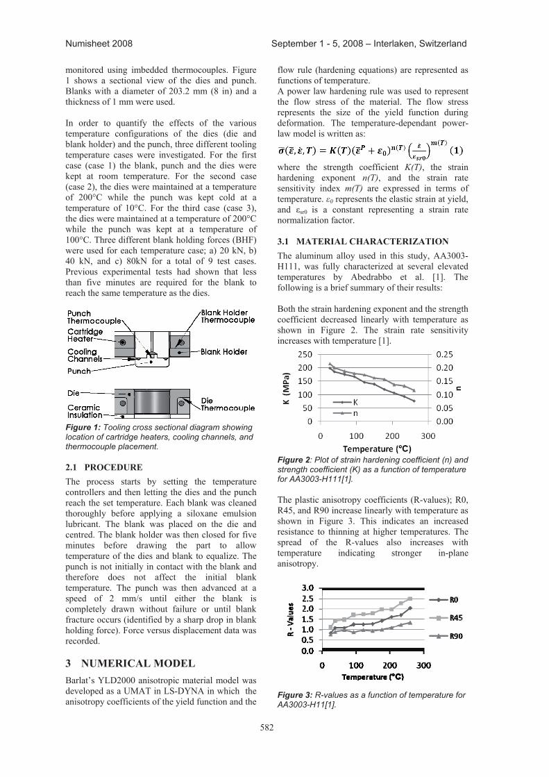
582


monitored using imbedded thermocouples. Figure 1 shows a sectional view of the dies and punch. Blanks with a diameter of 203.2 mm (8 in) and a thickness of 1 mm were used. In order to quantify the effects of the various temperature configurations of the dies (die and blank holder) and the punch, three different tooling temperature cases were investigated. For the first case (case 1) the blank, punch and the dies were kept at room temperature. For the second case (case 2), the dies were maintained at a temperature of 200°C while the punch was kept cold at a temperature of 10°C. For the third case (case 3), the dies were maintained at a temperature of 200°C while the punch was kept at a temperature of 100°C. Three different blank holding forces (BHF) were used for each temperature case; a) 20 kN, b) 40 kN, and c) 80kN for a total of 9 test cases. Previous experimental tests had shown that less than five minutes are required for the blank to reach the same temperature as the dies.

Figure 1: Tooling cross sectional diagram showing location of cartridge heaters, cooling channels, and thermocouple placement. 2.1 PROCEDURE The process starts by setting the temperature controllers and then letting the dies and the punch reach the set temperature. Each blank was cleaned thoroughly before applying a siloxane emulsion lubricant. The blank was placed on the die and centred. The blank holder was then closed for five minutes before drawing the part to allow temperature of the dies and blank to equalize. The punch is not initially in contact with the blank and therefore does not affect the initial blank temperature. The punch was then advanced at a speed of 2 mm/s until either the blank is completely drawn without failure or until blank fracture occurs (identified by a sharp drop in blank holding force). Force versus displacement data was recorded. 3 NUMERICAL MODEL Barlat’s YLD2000 anisotropic material model was developed as a UMAT in LS-DYNA in which the anisotropy coefficients of the yield function and the

flow rule (hardening equations) are represented as functions of temperature. A power law hardening rule was used to represent the flow stress of the material. The flow stress represents the size of the yield function during deformation. The temperature-dependant power-law model is written as:

where the strength coefficient K(T), the strain hardening exponent n(T), and the strain rate sensitivity index m(T) are expressed in terms of temperature. 0 represents the elastic strain at yield, and sr0 is a constant representing a strain rate normalization factor. 3.1 MATERIAL CHARACTERIZATION The aluminum alloy used in this study, AA3003-H111, was fully characterized at several elevated temperatures by Abedrabbo et al. [1]. The following is a brief summary of their results: Both the strain hardening exponent and the strength coefficient decreased linearly with temperature as shown in Figure 2. The strain rate sensitivity increases with temperature [1].

Figure 2: Plot of strain hardening coefficient (n) and strength coefficient (K) as a function of temperature for AA3003-H111[1]. The plastic anisotropy coefficients (R-values); R0, R45, and R90 increase linearly with temperature as shown in Figure 3. This indicates an increased resistance to thinning at higher temperatures. The spread of the R-values also increases with temperature indicating stronger in-plane anisotropy.

Figure 3: R-values as a function of temperature for AA3003-H11[1].

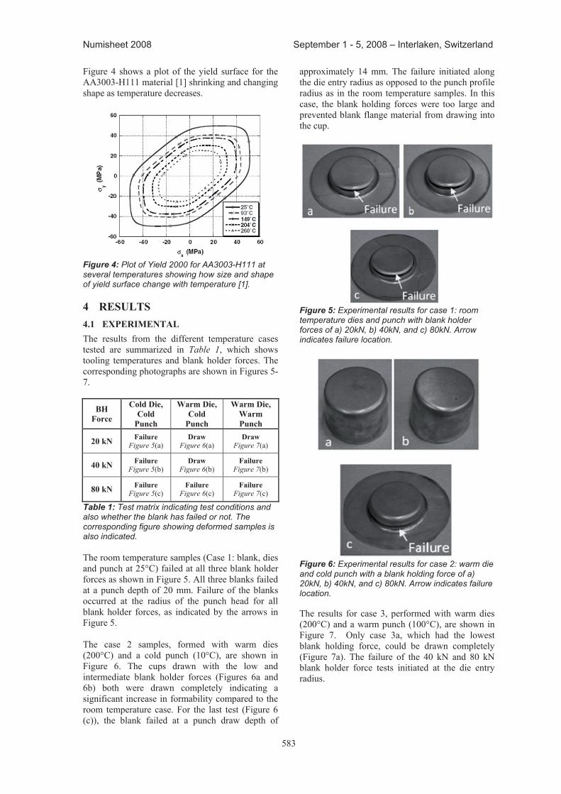
583


Figure 4 shows a plot of the yield surface for the AA3003-H111 material [1] shrinking and changing shape as temperature decreases.

Figure 4: Plot of Yield 2000 for AA3003-H111 at several temperatures showing how size and shape of yield surface change with temperature [1]. 4 RESULTS 4.1 EXPERIMENTAL The results from the different temperature cases tested are summarized in Table 1, which shows tooling temperatures and blank holder forces. The corresponding photographs are shown in Figures 5-7.

BH Force

Cold Die, Cold

Punch

Warm Die, Cold

Punch

Warm Die, Warm Punch

20 kN Failure Figure 5(a)

Draw Figure 6(a)

Draw Figure 7(a)

40 kN Failure Figure 5(b)

Draw Figure 6(b)

Failure Figure 7(b)

80 kN Failure Figure 5(c)

Failure Figure 6(c)

Failure Figure 7(c)

Table 1: Test matrix indicating test conditions and also whether the blank has failed or not. The corresponding figure showing deformed samples is also indicated. The room temperature samples (Case 1: blank, dies and punch at 25°C) failed at all three blank holder forces as shown in Figure 5. All three blanks failed at a punch depth of 20 mm. Failure of the blanks occurred at the radius of the punch head for all blank holder forces, as indicated by the arrows in Figure 5. The case 2 samples, formed with warm dies (200°C) and a cold punch (10°C), are shown in Figure 6. The cups drawn with the low and intermediate blank holder forces (Figures 6a and 6b) both were drawn completely indicating a significant increase in formability compared to the room temperature case. For the last test (Figure 6 (c)), the blank failed at a punch draw depth of

approximately 14 mm. The failure initiated along the die entry radius as opposed to the punch profile radius as in the room temperature samples. In this case, the blank holding forces were too large and prevented blank flange material from drawing into the cup.

Figure 5: Experimental results for case 1: room temperature dies and punch with blank holder forces of a) 20kN, b) 40kN, and c) 80kN. Arrow indicates failure location.

Figure 6: Experimental results for case 2: warm die and cold punch with a blank holding force of a) 20kN, b) 40kN, and c) 80kN. Arrow indicates failure location. The results for case 3, performed with warm dies (200°C) and a warm punch (100°C), are shown in Figure 7. Only case 3a, which had the lowest blank holding force, could be drawn completely (Figure 7a). The failure of the 40 kN and 80 kN blank holder force tests initiated at the die entry radius.

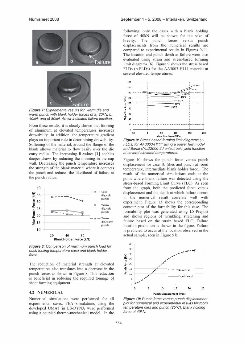
584


Figure 7: Experimental results for warm die and warm punch with blank holder forces of a) 20kN, b) 40kN, and c) 80kN. Arrow indicates failure location.

From these results, it is clearly shown that forming of aluminum at elevated temperatures increases drawability. In addition, the temperature gradient plays an important role in determining drawability. Softening of the material, around the flange of the blank allows material to flow easily over the die entry radius. The increasing R-values [1] enables deeper draws by reducing the thinning in the cup wall. Decreasing the punch temperature increases the strength of the blank material where it contacts the punch and reduces the likelihood of failure at the punch radius.

Figure 8: Comparison of maximum punch load for each tooling temperature case and blank holder force. The reduction of material strength at elevated temperatures also translates into a decrease in the punch forces as shown in Figure 8. This reduction is beneficial in reducing the required tonnage of sheet forming equipment. 4.2 NUMERICAL Numerical simulations were performed for all experimental cases. FEA simulations using the developed UMAT in LS-DYNA were performed using a coupled thermo-mechanical model. In the

following, only the cases with a blank holding force of 40kN will be shown for the sake of brevity. The punch forces versus punch displacements from the numerical results are compared to experimental results in Figures 9-11. The location and punch depth at failure were also evaluated using strain and stress-based forming limit diagrams [6]. Figure 9 shows the stress based FLDs ( -FLDs) for the AA3003-H111 material at several elevated temperatures.

Figure 9: Stress based forming limit diagrams ( -FLDs) for AA3003-H111 using a power law model and Barlat’sYLD2000-2d anisotropic yield function at several elevated temperatures.

Figure 10 shows the punch force versus punch displacement for case 1b (dies and punch at room temperature, intermediate blank holder force). The result of the numerical simulations ends at the point where blank failure was detected using the stress-based Forming Limit Curve (FLC). As seen from the graph, both the predicted force versus displacement and the depth at which failure occurs in the numerical result correlate well with experiment. Figure 13 shows the corresponding contour plot of the formability for this case. The formability plot was generated using LS-Prepost and shows regions of wrinkling, stretching and failure based on the strain based FLC. Failure location prediction is shown in the figure. Failure is predicted to occur at the location observed in the actual sample, seen in Figure 5 b.

Figure 10: Punch force versus punch displacement plot for numerical and experimental results for room temperature dies and punch (25°C). Blank holding force at 40kN.

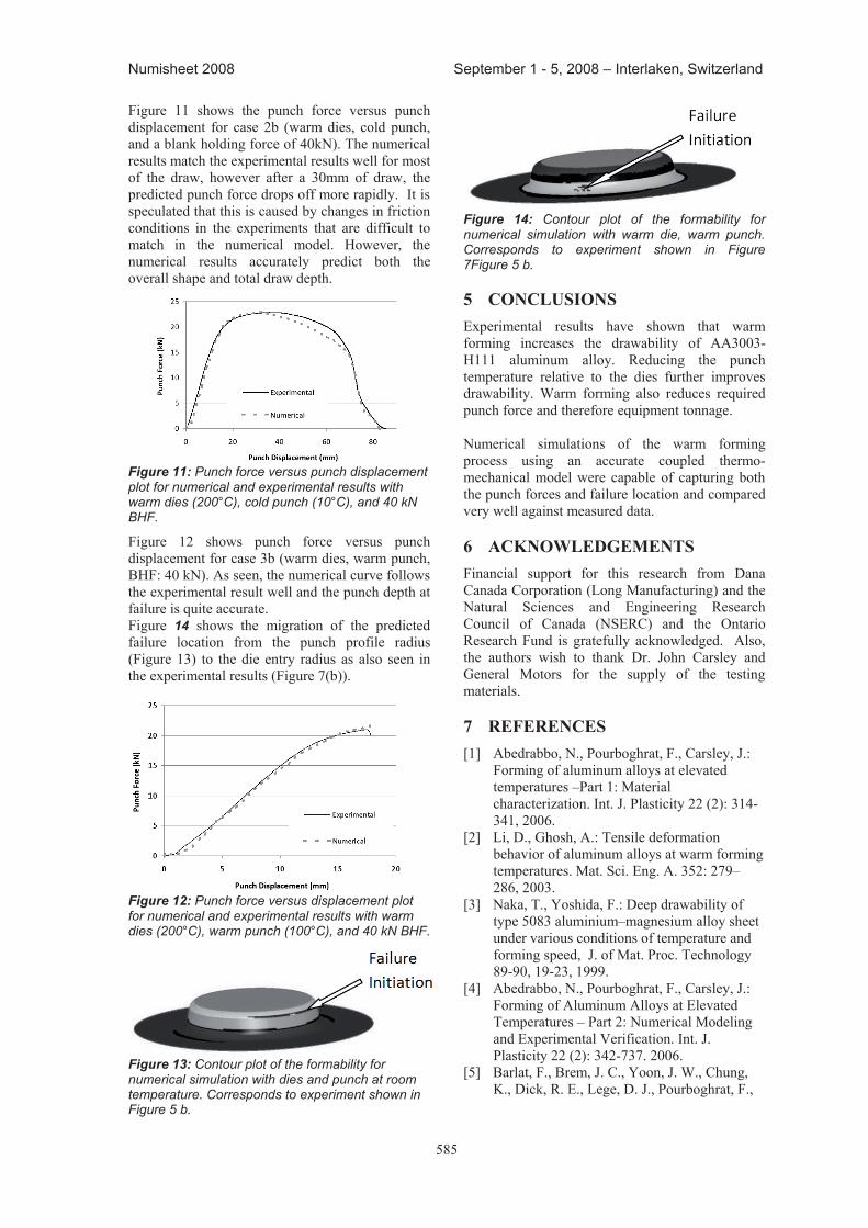
585


Figure 11 shows the punch force versus punch displacement for case 2b (warm dies, cold punch, and a blank holding force of 40kN). The numerical results match the experimental results well for most of the draw, however after a 30mm of draw, the predicted punch force drops off more rapidly. It is speculated that this is caused by changes in friction conditions in the experiments that are difficult to match in the numerical model. However, the numerical results accurately predict both the overall shape and total draw depth.

Figure 11: Punch force versus punch displacement plot for numerical and experimental results with warm dies (200°C), cold punch (10°C), and 40 kN BHF.

Figure 12 shows punch force versus punch displacement for case 3b (warm dies, warm punch, BHF: 40 kN). As seen, the numerical curve follows the experimental result well and the punch depth at failure is quite accurate. Figure 14 shows the migration of the predicted failure location from the punch profile radius (Figure 13) to the die entry radius as also seen in the experimental results (Figure 7(b)).

Figure 12: Punch force versus displacement plot for numerical and experimental results with warm dies (200°C), warm punch (100°C), and 40 kN BHF.

Figure 13: Contour plot of the formability for numerical simulation with dies and punch at room temperature. Corresponds to experiment shown in Figure 5 b.

Figure 14: Contour plot of the formability for numerical simulation with warm die, warm punch. Corresponds to experiment shown in Figure 7Figure 5 b. 5 CONCLUSIONS Experimental results have shown that warm forming increases the drawability of AA3003-H111 aluminum alloy. Reducing the punch temperature relative to the dies further improves drawability. Warm forming also reduces required punch force and therefore equipment tonnage. Numerical simulations of the warm forming process using an accurate coupled thermo-mechanical model were capable of capturing both the punch forces and failure location and compared very well against measured data. 6 ACKNOWLEDGEMENTS Financial support for this research from Dana Canada Corporation (Long Manufacturing) and the Natural Sciences and Engineering Research Council of Canada (NSERC) and the Ontario Research Fund is gratefully acknowledged. Also, the authors wish to thank Dr. John Carsley and General Motors for the supply of the testing materials. 7 REFERENCES [1] Abedrabbo, N., Pourboghrat, F., Carsley, J.:

Forming of aluminum alloys at elevated temperatures –Part 1: Material characterization. Int. J. Plasticity 22 (2): 314-341, 2006.

[2] Li, D., Ghosh, A.: Tensile deformation behavior of aluminum alloys at warm forming temperatures. Mat. Sci. Eng. A. 352: 279–286, 2003.

[3] Naka, T., Yoshida, F.: Deep drawability of type 5083 aluminium–magnesium alloy sheet under various conditions of temperature and forming speed, J. of Mat. Proc. Technology 89-90, 19-23, 1999.

[4] Abedrabbo, N., Pourboghrat, F., Carsley, J.: Forming of Aluminum Alloys at Elevated Temperatures – Part 2: Numerical Modeling and Experimental Verification. Int. J. Plasticity 22 (2): 342-737. 2006.

[5] Barlat, F., Brem, J. C., Yoon, J. W., Chung, K., Dick, R. E., Lege, D. J., Pourboghrat, F.,

586


Choi, S. H., and Chu, E.: Int. J. of Plasticity 19: 1297-1319, 2003.

[6] Stoughton, T. B.: Stress-based Forming Limits in Sheet Metal Forming. J. Eng. Mat. Tech., 123:417- 422, 2001.

587


____________________* Corresponding author: Via Venezia 1, 35131, Padova, Italy, Tel: +39 049 8276819, Fax: +39 049 8276816, [email protected]

CaLIBratION OF NUMerICaL SIMULatION FOr hOt StaMpING

a. turetta1, S. Fanini*1, a. Ghiotti1, S. Bruschi2

1DIMEG, Univ. of Padova, Via Venezia 1, 35131, Padova, Italy 2DIMS, Univ. of Trento, Via Mesiano 77, 38050, Trento, Italy

aBStraCt: In the last few years, sheet metal working operations at elevated temperatures have gained much importance due to the possibility of producing components characterized by high strength-to-mass ratio. In particular, the hot stamping of ultra high strength quenchenable steels is nowadays widely utilized in the automotive industry to produce structural parts with enhanced crash characteristics and geometrical accuracy. The choice of the most appropriate process parameters requires the utilization of FE-based codes where the process has to be represented by a fully coupled thermo-mechanical-metallurgical model. The accurate calibration of such a model, in terms of material behaviour, boundary conditions, phase transformation and formability limits, is then a strong requirement for the results reliability in the numerical simulations of sheet metal forming processes and offer noticeable time and cost savings to car designers and producers. In its first part, the paper presents the requirements in terms of implemented data that a fully coupled thermo-mechanical-metallurgical model must satisfy in order to accurately reproduce those phenomena characterising hot stamping. Testing procedures to gain material and interface data together with relevant results are then presented. Finally, available numerical models are analysed and discussed depending on the phenomena that they are capable to represent.

KeYWOrDS: Sheet Metal Forming, Hot stamping, FEM, Calibration

1 INtrODUCtIONIn the last years the main targets of automotive industry have been represented by (i) the reduction of the vehicles environmental impact (pollutions, fuel consumption, CO2 emission), (ii) the increase of safety (impact absorption performance, crash resistance, pedestrian safety, etc.), and (iii) the improved accuracy and quality for easier, cheaper and more reliable joining and assembly of final components. These requirements have forced and are still forcing car manufacturers to a continuous search for new solutions, leading to the most significant evolution and innovation in sheet metal forming technologies. Different types of materials, both metallic and non-metallic, are utilised for such purposes. As regards the metallic ones, aluminium alloys and different steels grades are the most commonly utilised in body-in-white components and reinforcements beams, while the introduction of high strength quenchenable steels (HSS) has represented an innovative solution to increase the strength-to-mass ratio of sheet metal components. In particular, in order to fully exploit their

characteristics, HSS must be deformed at elevated temperature – to enhance their formability – and simultaneously quenched – to obtain a high strength martensitic microstructure in the component at room temperature [1-4]. In the hot stamping, or press hardening process, the steel blank is heated up above austenitization temperature, then transferred to the press where deformation takes place simultaneously with quenching inside the forming dies in order to achieve a fully martensitic microstructure. Compared with traditional sheet metal forming operations, the proper design of hot stamping process chain requires a deep knowledge of both interface phenomena and material behaviour at high temperature. In particular, the choice of the most suitable process parameters of the forming and the cooling phases requires the utilization of FE-based codes where the process has to be represented by a fully coupled thermo-mechanical-metallurgical model. Such a model has to be accurately calibrated and validated, by means of experimental techniques and numerical inverse

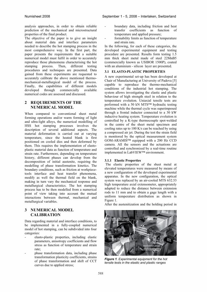
588


analysis approaches, in order to obtain reliable prediction of the mechanical and microstructural properties of the final product. The objective of the paper is to give an insight about material data and interface parameters needed to describe the hot stamping process in the most comprehensive way. In the first part, the paper presents the requirements that a suitable numerical model must fulfil in order to accurately reproduce those phenomena characterising the hot stamping process. Then, different testing procedures and techniques are presented. Data gained from these experiments are requested to accurately calibrate the above mentioned thermo-mechanical-metallurgical model of the process. Finally, the capabilities of different models developed through commercially available numerical codes are assessed and discussed.

2 reQUIreMeNtS OF the NUMerICaL MODeL

When compared to conventional sheet metal forming operations and/or warm forming of light and ultra-light alloys, the numerical modelling of HSS hot stamping processes involves the description of several additional aspects. The material deformation is carried out at varying temperature, since the heated blank is first positioned on cooled dies and then deformed by them. This requires the implementation of elasto-plastic material data as function of temperature and strain rate. Furthermore, depending on temperature history, different phases can develop from the decomposition of initial austenite, requiring the modelling of phase transformation kinetics. The boundary conditions, such as friction at workpiece-tools interface and heat transfer phenomena, modify as well the thermal field on the blank, making in turn vary the mechanical response and metallurgical characteristics. The hot stamping process has to be then modelled from a numerical point of view taking into account the mutual interactions between thermal, mechanical and metallurgical variables.

3 NUMerICaL MODeL CaLIBratION

Data regarding material and interface conditions, to be implemented in a fully-coupled numerical model of hot stamping, can be subdivided into four categories:- elasto-plastic properties, including elastic

parameters, anisotropy coefficients and flow stress as function of temperature and strain rate;

- phase transformation data, including phase transformation plasticity coefficients, strains of phase transformation and shift of CCT curves due to applied stress;

- boundary data, including friction and heat transfer coefficients as function of temperature and applied pressure;

- formability limits as function of temperature and strain rate.

In the following, for each of these categories, the developed experimental equipment and testing procedure are presented. Results form testing 1.5 mm thick sheet metal made of steel 22MnB5 (commercially known as USIBOR 1500P), coated with an aluminium - silicon layer are presented. 3.1 eLaStO-pLaStIC prOpertIeS A new experimental set-up has been developed at Chair of Manufacturing at University of Padova [5] capable to reproduce the thermo-mechanical conditions of the industrial hot stamping. The system allows investigating the elastic and plastic behaviour of high strength steel in relation to the temperature evolution. Uniaxial tensile tests are performed with a 50 kN MTS™ hydraulic testing machine while the thermal cycle was superimposed through a frontal inductor connected to a 30 kW inductive heating system. Temperature evolution is controlled by a K-type thermocouple spot-welded in the centre of the sheet metal specimen and cooling rates up to 100 K/s can be reached by using a compressed air jet. During the test the strain field is monitored by the optical measurement system GOM-ARAMIS™ equipped with a 200 Hz CCD camera. All the sensors and the actuations are controlled and synchronized by a real-time routine implemented in LabVIEW™ environment.

3.1.1 elastic properties The elastic properties of the sheet metal at elevated temperatures were measured by means of a new configuration of the developed experimental apparatus. In the new configuration, the optical system was replaced by an air-cooled MTS 632.53 high temperature axial extensometer, appropriately adapted to reduce the distance between extension rods to 11 mm and to obtain a gage length with a uniform temperature distribution as shown in Figure 1. After the austenitization and the holding period in

Figure 1. Experimental equipment for the hot tensile tests in the elastic and plastic ranges

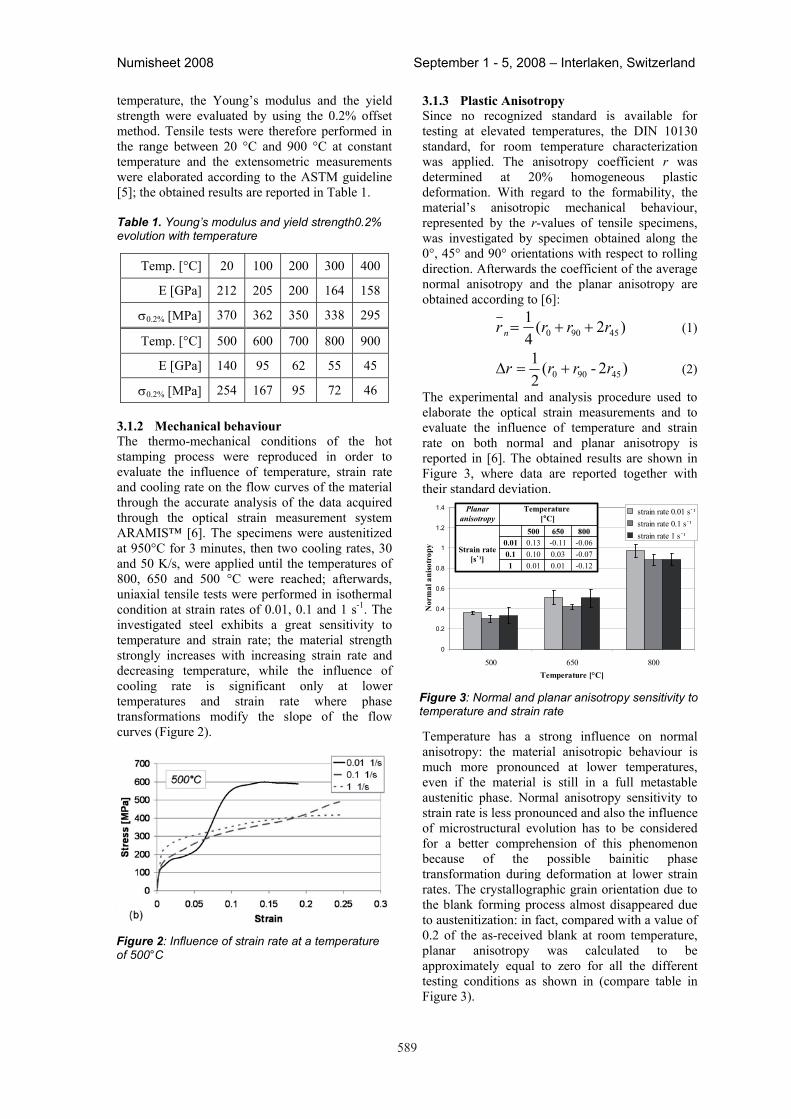
589


temperature, the Young’s modulus and the yield strength were evaluated by using the 0.2% offset method. Tensile tests were therefore performed in the range between 20 °C and 900 °C at constant temperature and the extensometric measurements were elaborated according to the ASTM guideline [5]; the obtained results are reported in Table 1.

Table 1. Young’s modulus and yield strength0.2% evolution with temperature

Temp. [°C] 20 100 200 300 400

E [GPa] 212 205 200 164 158

0.2% [MPa] 370 362 350 338 295

Temp. [°C] 500 600 700 800 900

E [GPa] 140 95 62 55 45

0.2% [MPa] 254 167 95 72 46

3.1.2 Mechanical behaviour The thermo-mechanical conditions of the hot stamping process were reproduced in order to evaluate the influence of temperature, strain rate and cooling rate on the flow curves of the material through the accurate analysis of the data acquired through the optical strain measurement system ARAMIS™ [6]. The specimens were austenitized at 950°C for 3 minutes, then two cooling rates, 30 and 50 K/s, were applied until the temperatures of 800, 650 and 500 °C were reached; afterwards, uniaxial tensile tests were performed in isothermal condition at strain rates of 0.01, 0.1 and 1 s-1. The investigated steel exhibits a great sensitivity to temperature and strain rate; the material strength strongly increases with increasing strain rate and decreasing temperature, while the influence of cooling rate is significant only at lower temperatures and strain rate where phase transformations modify the slope of the flow curves (Figure 2).

Figure 2: Influence of strain rate at a temperature of 500°C

3.1.3 plastic anisotropy Since no recognized standard is available for testing at elevated temperatures, the DIN 10130 standard, for room temperature characterization was applied. The anisotropy coefficient r was determined at 20% homogeneous plastic deformation. With regard to the formability, the material’s anisotropic mechanical behaviour, represented by the r-values of tensile specimens, was investigated by specimen obtained along the 0°, 45° and 90° orientations with respect to rolling direction. Afterwards the coefficient of the average normal anisotropy and the planar anisotropy are obtained according to [6]:

)2(41

45900 rrrr n (1)

)2-(21

45900 rrrr (2)

The experimental and analysis procedure used to elaborate the optical strain measurements and to evaluate the influence of temperature and strain rate on both normal and planar anisotropy is reported in [6]. The obtained results are shown in Figure 3, where data are reported together with their standard deviation.

0

0.2

0.4

0.6

0.8

1

1.2

1.4

500 650 800temperature [°C]

Nor

mal

ani

sotr

opy

strain rate 0.01 s˙¹ strain rate 0.1 s˙¹ strain rate 1 s˙¹

-0.120.010.011-0.070.030.100.1-0.06-0.110.130.01

Strain rate [s˙¹]

800650500

temperature[°C]

Planar anisotropy

-0.120.010.011-0.070.030.100.1-0.06-0.110.130.01

Strain rate [s˙¹]

800650500

temperature[°C]

Planar anisotropy

Figure 3: Normal and planar anisotropy sensitivity to temperature and strain rate

Temperature has a strong influence on normal anisotropy: the material anisotropic behaviour is much more pronounced at lower temperatures, even if the material is still in a full metastable austenitic phase. Normal anisotropy sensitivity to strain rate is less pronounced and also the influence of microstructural evolution has to be considered for a better comprehension of this phenomenon because of the possible bainitic phase transformation during deformation at lower strain rates. The crystallographic grain orientation due to the blank forming process almost disappeared due to austenitization: in fact, compared with a value of 0.2 of the as-received blank at room temperature, planar anisotropy was calculated to be approximately equal to zero for all the different testing conditions as shown in (compare table in Figure 3).

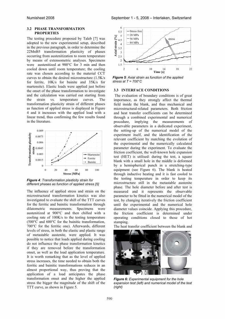
590


3.2 phaSe traNSFOrMatION prOpertIeS

The testing procedure proposed by Taleb [7] was adopted to the new experimental setup, described in the previous paragraph, in order to determine the 22MnB5 transformation plasticity of phases occurring from austenitization to room temperature by means of extensometric analyses. Specimens were austenitized at 900°C for 3 min and then cooled down until room temperature; the cooling rate was chosen according to the material CCT curves to obtain the desired microstructure (1.5K/s for ferrite, 10K/s for bainite and 35K/s for martensite). Elastic loads were applied just before the onset of the phase transformation to investigate and the calculation was carried out starting from the strain vs. temperature curves. The transformation plasticity strain of different phases as function of applied stress is displayed in Figure 4 and it increases with the applied load with a linear trend, thus confirming the few results found in the literature.

0

0.0015

0.003

0.0045

0.006

0.0075

0.009

0 20 40 60 80 100Stress [Mpa]

tran

sfor

mat

ion

plas

ticity

st

rain

s

MartensiteFerriteBainite

Figure 4: Transformation plasticity strain for different phases as function of applied stress [5]

The influence of applied stress and strain on the microstructural transformation kinetics was also investigated to evaluate the shift of the TTT curves for the ferritic and bainitic transformation through dilatometric measurements. Specimens were austenitized at 900°C and then chilled with a cooling rate of 100K/s to the testing temperature (500°C and 600°C for the bainitic transformation, 700°C for the ferritic one). Afterwards, different levels of stress, in both the elastic and plastic range of metastable austenite, were applied. It was possible to notice that loads applied during cooling do not influence the phase transformation kinetics if they are removed before the transformation onset, as well as the load application temperature. It is worth remarking that as the level of applied stress increases, the time needed to obtain both the ferritic and bainitic transformations reduces in an almost proportional way, thus proving that the application of a load anticipates the phase transformation onset and the higher the applied stress the bigger the magnitude of the shift of the TTT curve, as shown in Figure 5.

1.52

2.53

3.54

4.55

5.56

2 6 10 14 18 22time [s]

axi

al st

rain

[%]

Stress free28 MPa56 MPa84 MPa

stress

Figure 5: Axial strain as function of the applied stress at T = 700°C

3.3 INterFaCe CONDItIONS The evaluation of boundary conditions is of great importance, as they strongly affect the thermal field inside the blank, and thus mechanical and microstructural-related parameters. Both friction and heat transfer coefficients can be determined through a combined experimental and numerical procedure, implying the measurements of observable parameters in a dedicated experiment, the setting-up of the numerical model of the experiment itself, and the identification of the relevant coefficient by matching the evolution of the experimental and the numerically calculated parameter during the experiment. To evaluate the friction coefficient, the well-known hole expansion test (HET) is utilised: during the test, a square blank with a small hole in the middle is deformed by a hemispherical punch in a stretching-type equipment (see Figure 6). The blank is heated through inductive heating and it is fast cooled to the testing temperature in order to keep its microstructure still in the metastable austenite phase. The hole diameter before and after test is measured and it represents the observable parameter to be fitted in the numerical model of the test, by changing iteratively the friction coefficient until the experimental and the numerical hole diameter values coincide. Applying this procedure, the friction coefficient is determined under operating conditions closed to those of hot stamping. The heat transfer coefficient between the blank and

Figure 6: Experimental equipment for the hole expansion test (left) and numerical model of the test (right)

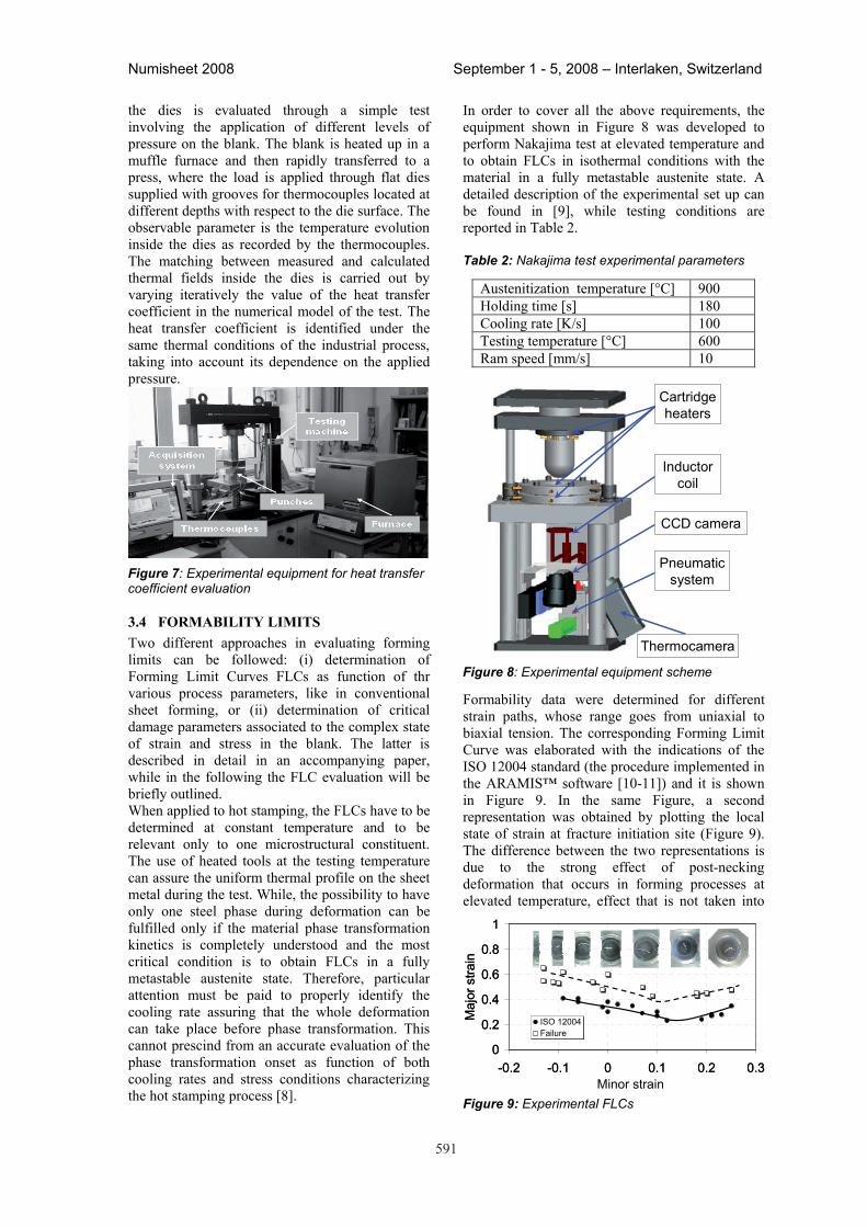
591


the dies is evaluated through a simple test involving the application of different levels of pressure on the blank. The blank is heated up in a muffle furnace and then rapidly transferred to a press, where the load is applied through flat dies supplied with grooves for thermocouples located at different depths with respect to the die surface. The observable parameter is the temperature evolution inside the dies as recorded by the thermocouples. The matching between measured and calculated thermal fields inside the dies is carried out by varying iteratively the value of the heat transfer coefficient in the numerical model of the test. The heat transfer coefficient is identified under the same thermal conditions of the industrial process, taking into account its dependence on the applied pressure.

Figure 7: Experimental equipment for heat transfer coefficient evaluation

3.4 FOrMaBILItY LIMItS Two different approaches in evaluating forming limits can be followed: (i) determination of Forming Limit Curves FLCs as function of thr various process parameters, like in conventional sheet forming, or (ii) determination of critical damage parameters associated to the complex state of strain and stress in the blank. The latter is described in detail in an accompanying paper, while in the following the FLC evaluation will be briefly outlined. When applied to hot stamping, the FLCs have to be determined at constant temperature and to be relevant only to one microstructural constituent. The use of heated tools at the testing temperature can assure the uniform thermal profile on the sheet metal during the test. While, the possibility to have only one steel phase during deformation can be fulfilled only if the material phase transformation kinetics is completely understood and the most critical condition is to obtain FLCs in a fully metastable austenite state. Therefore, particular attention must be paid to properly identify the cooling rate assuring that the whole deformation can take place before phase transformation. This cannot prescind from an accurate evaluation of the phase transformation onset as function of both cooling rates and stress conditions characterizing the hot stamping process [8].

In order to cover all the above requirements, the equipment shown in Figure 8 was developed to perform Nakajima test at elevated temperature and to obtain FLCs in isothermal conditions with the material in a fully metastable austenite state. A detailed description of the experimental set up can be found in [9], while testing conditions are reported in Table 2.

Table 2: Nakajima test experimental parameters

Austenitization temperature [°C] 900 Holding time [s] 180 Cooling rate [K/s] 100 Testing temperature [°C] 600 Ram speed [mm/s] 10

Cartridge heaters

Inductorcoil

CCD camera

Pneumatic system

Thermocamera

Figure 8: Experimental equipment scheme

Formability data were determined for different strain paths, whose range goes from uniaxial to biaxial tension. The corresponding Forming Limit Curve was elaborated with the indications of the ISO 12004 standard (the procedure implemented in the ARAMIS™ software [10-11]) and it is shown in Figure 9. In the same Figure, a second representation was obtained by plotting the local state of strain at fracture initiation site (Figure 9). The difference between the two representations is due to the strong effect of post-necking deformation that occurs in forming processes at elevated temperature, effect that is not taken into

0

0.2

0.4

0.6

0.8

1

-0.2 -0.1 0 0.1 0.2 0.3Minor strain

Maj

or s

train

ISO 12004Failure

0

0.2

0.4

0.6

0.8

1

-0.2 -0.1 0 0.1 0.2 0.3Minor strain

Maj

or s

train

ISO 12004Failure

Figure 9: Experimental FLCs

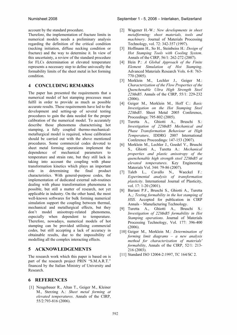
592


account by the standard procedure. Therefore, the implementation of fracture limits in numerical models needs a preliminary analysis regarding the definition of the critical condition (necking initiation, diffuse necking condition or fracture) and the way to determine it. In view of this uncertainty, a review of the standard procedure for FLCs determination at elevated temperature represents a necessary step to define univocally the formability limits of the sheet metal in hot forming condition.

4 CONCLUDING reMarKS The paper has presented the requirements that a numerical model of hot stamping processes must fulfil in order to provide as much as possible accurate results. These requirements have led to the development and setting-up of several testing procedures to gain the data needed for the proper calibration of the numerical model. To accurately describe those phenomena characterising hot stamping, a fully coupled thermo-mechanical-metallurgical model is required, whose calibration should be carried out with the above mentioned procedures. Some commercial codes devoted to sheet metal forming operations implement the dependence of mechanical parameters to temperature and strain rate, but they still lack in taking into account the coupling with phase transformation kinetics which plays an important role in determining the final product characteristics. With general-purpose codes, the implementation of dedicated external sub-routines dealing with phase transformation phenomena is possible, but still a matter of research, not yet applicable in industry. On the other hand, the most well-known softwares for bulk forming numerical simulation support the coupling between thermal, mechanical and metallurgical effects, but they don’t model anisotropy-related phenomena, especially when dependent to temperature. Therefore, nowadays, numerical models of hot stamping can be provided utilising commercial codes, but still accepting a lack of accuracy in obtainable results, due to the impossibility of modelling all the complex interacting effects.

5 aCKNOWLeDGeMeNtS The research work which this paper is based on is part of the research project PRIN “S.M.A.R.T.” financed by the Italian Ministry of University and Research.

6 reFereNCeS [1] Neugebauer R., Altan T., Geiger M., Kleiner

M., Sterzing A.: Sheet metal forming at elevated temperatures. Annals of the CIRP, 55/2:793-816 (2006).

[2] Wagener H.-W.: New developments in sheet metalforming: sheet materials, tools and machinery. Journal of Materials Processing Technology, vol. 72: 342-357 (1997).

[3] Hoffmann H., So H., Steinbeiss H.: Design of Hot Stamping Tools with Cooling System.Annals of the CIRP, 56/1: 262-272 (2007).

[4] Hein P.: A Global Approach of the Finite Element Simulation of Hot Stamping.Advanced Materials Research Vols. 6-8: 763-770 (2005).

[3] Merklein M., Lechler J., Geiger M.: Characterization of the Flow Properties of the Quenchenable Ultra High Strength Steel 22MnB5. Annals of the CIRP, 55/1: 229-232 (2006).

[4] Geiger M., Merklein M., Hoff C.: Basic Investigation on the Hot Stamping Steel 22MnB5. Sheet Metal 2005 Conference, Proceedings: 795-802 (2005).

[5] Turetta A., Ghiotti A., Bruschi S.: Investigation of 22MnB5 Mechanical and Phase Transformation Behaviour at High Temperature, IDDRG 2007 International Conference Proceedings: 147-153 (2007).

[6] Merklein M., Lechler J., Goedel V., Bruschi S., Ghiotti A., Turetta A.: Mechanical properties and plastic anisotropy of the quenchenable high strength steel 22MnB5 at elevated temperatures. Key Engineering Materials Vol. 344: 79-86 (2007).

[7] Taleb L., Cavallo N., Waeckel F.: Experimental analysis of transformation plasticity. International Journal of Plasticity, vol. 17: 1-20 (2001).

[8] Bariani P.F., Bruschi S., Ghiotti A., Turetta A.,: Testing formability in the hot stamping of HSS. Accepted for publication in CIRP Annals – Manufacturing Technology.

[9] Turetta A., Ghiotti A., Bruschi S.: Investigation of 22MnB5 formability in Hot Stamping operations. Journal of Materials Processing Technology, Vol. 177: 396-400 (2006).

[10] Geiger M., Merklein M.: Determination of forming limit diagrams – a new analysis method for characterization of materials' formability, Annals of the CIRP, 52/1: 213-216 (2003).

[11] Standard ISO 12004-2:1997, TC 164/SC 2.

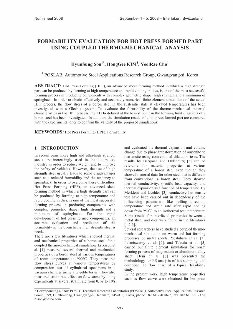
593


____________________ * Corresponding author: POSCO Technical Research Laboratories (POSLAB), Automotive Steel Applications Research Group, 699, Gumho-dong, Gwangyang-si, Jeonnam, 545-090, Korea, phone +82 61 790 8675, fax +82 61 790 9370, [email protected]

FOrMaBILItY eVaLUatION FOr hOt preSS FOrMeD part USING COUpLeD therMO-MeChaNICaL aNaYSIS

hyunSung Son1*, hongGee KIM1, Yeolrae Cho1

1 POSLAB, Automotive Steel Applications Research Group, Gwangyang-si, Korea

aBStraCt: Hot Press Forming (HPF), an advanced sheet forming method in which a high strength part can be produced by forming at high temperature and rapid cooling in dies, is one of the most successful forming process in producing components with complex geometric shape, high strength and a minimum of springback. In order to obtain effectively and accurately numerical finite element simulations of the actual HPF process, the flow stress of a boron steel in the austenitic state at elevated temperatures has been investigated with a Gleeble system. To evaluate the formability of the thermo-mechanical material characteristics in the HPF process, the FLDo defined at the lowest point in the forming limit diagrams of a boron steel has been investigated. In addition, the simulation results of a hot press formed part are compared with the experimental ones to confirm the validity of the proposed simulations.

KeYWOrDS: Hot Press Forming (HPF), Formability

1 INtrODUCtION In recent years more high and ultra-high strength steels are increasingly used in the automotive industry in order to reduce weight and to improve the safety of vehicles. However, the use of high strength steel usually leads to some disadvantages such as a reduced formability and the tendency to springback. In order to overcome these difficulties, Hot Press Forming (HPF), an advanced sheet forming method in which a high strength part can be produced by forming at high temperature and rapid cooling in dies, is one of the most successful forming process in producing components with complex geometric shape, high strength and a minimum of springback. For the rapid development of hot press formed components, an accurate evaluation and prediction of the formability in the quenchable high strength steel is needed. There are a few literatures which showed thermal and mechanical properties of a boron steel for a coupled thermo-mechanical simulation. Eriksson et al. [1] measured several thermal and mechanical properties of a boron steel at various temperatures of room temperature to 900°C. They measured flow stress curves at various temperatures by compression test of cylindrical specimens in a vacuum chamber using a Gleeble tester. They also measured strain rate effect on flow stress by doing experiments at several strain rate from 0.1/s to 10/s,

and evaluated the thermal expansion and volume change due to phase transformation of austenite to martensite using conventional dilatation tests. The results by Bergman and Oldenburg [2] can be referable for material properties at various temperature of a boron steel even though they showed material data for other steel that is different from conventional a boron steel. They showed thermal conductivity, specific heat capacity, and thermal expansion as a function of temperature. By Merklein and Lechler [3], conductive hot tensile test have been carried out in dependency of the influencing parameters like rolling direction, temperature and strain rate after rapid cooling down from 950 to an isothermal test temperature. Some results for interfacial properties between a metal sheet and dies were found in the literatures [4,5,6]. Several researchers have studied a coupled thermo-mechanical simulation on warm and hot forming processes of metal sheets. Yoshihara et al. [7], Palaniswamy et al. [4], and Takuda et al. [5] carried out finite element simulation for warm forming process of magnesium or aluminium alloy sheet. Hein et al. [8] was presented the methodology for FE-analysis of hot stamping, and described the flow chart of a typical feasibility study. In the present work, high temperature properties such as flow curve were obtained for hot press

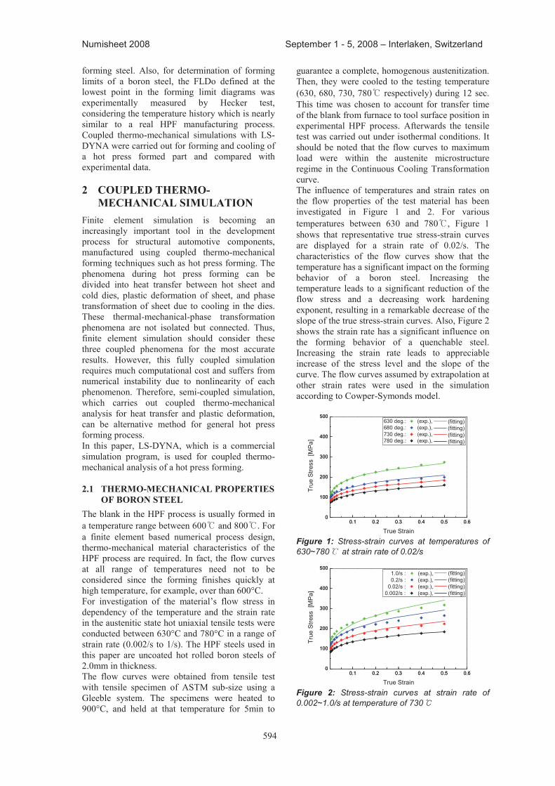
594


forming steel. Also, for determination of forming limits of a boron steel, the FLDo defined at the lowest point in the forming limit diagrams was experimentally measured by Hecker test, considering the temperature history which is nearly similar to a real HPF manufacturing process. Coupled thermo-mechanical simulations with LS-DYNA were carried out for forming and cooling of a hot press formed part and compared with experimental data.

2 COUpLeD therMO-MeChaNICaL SIMULatION

Finite element simulation is becoming an increasingly important tool in the development process for structural automotive components, manufactured using coupled thermo-mechanical forming techniques such as hot press forming. The phenomena during hot press forming can be divided into heat transfer between hot sheet and cold dies, plastic deformation of sheet, and phase transformation of sheet due to cooling in the dies. These thermal-mechanical-phase transformation phenomena are not isolated but connected. Thus, finite element simulation should consider these three coupled phenomena for the most accurate results. However, this fully coupled simulation requires much computational cost and suffers from numerical instability due to nonlinearity of each phenomenon. Therefore, semi-coupled simulation, which carries out coupled thermo-mechanical analysis for heat transfer and plastic deformation, can be alternative method for general hot press forming process. In this paper, LS-DYNA, which is a commercial simulation program, is used for coupled thermo-mechanical analysis of a hot press forming.

2.1 therMO-MeChaNICaL prOpertIeS OF BOrON SteeL

The blank in the HPF process is usually formed in a temperature range between 600 and 800 . For a finite element based numerical process design, thermo-mechanical material characteristics of the HPF process are required. In fact, the flow curves at all range of temperatures need not to be considered since the forming finishes quickly at high temperature, for example, over than 600°C. For investigation of the material’s flow stress in dependency of the temperature and the strain rate in the austenitic state hot uniaxial tensile tests were conducted between 630°C and 780°C in a range of strain rate (0.002/s to 1/s). The HPF steels used in this paper are uncoated hot rolled boron steels of 2.0mm in thickness. The flow curves were obtained from tensile test with tensile specimen of ASTM sub-size using a Gleeble system. The specimens were heated to 900°C, and held at that temperature for 5min to

guarantee a complete, homogenous austenitization. Then, they were cooled to the testing temperature (630, 680, 730, 780 respectively) during 12 sec. This time was chosen to account for transfer time of the blank from furnace to tool surface position in experimental HPF process. Afterwards the tensile test was carried out under isothermal conditions. It should be noted that the flow curves to maximum load were within the austenite microstructure regime in the Continuous Cooling Transformation curve. The influence of temperatures and strain rates on the flow properties of the test material has been investigated in Figure 1 and 2. For various temperatures between 630 and 780 , Figure 1 shows that representative true stress-strain curves are displayed for a strain rate of 0.02/s. The characteristics of the flow curves show that the temperature has a significant impact on the forming behavior of a boron steel. Increasing the temperature leads to a significant reduction of the flow stress and a decreasing work hardening exponent, resulting in a remarkable decrease of the slope of the true stress-strain curves. Also, Figure 2 shows the strain rate has a significant influence on the forming behavior of a quenchable steel. Increasing the strain rate leads to appreciable increase of the stress level and the slope of the curve. The flow curves assumed by extrapolation at other strain rates were used in the simulation according to Cowper-Symonds model.

0.1 0.2 0.3 0.4 0.5 0.60

100

200

300

400

500

0.1 0.2 0.3 0.4 0.5 0.60

100

200

300

400

500

True

Stre

ss [

MPa

]

True Strain

(fitting) (fitting) (fitting) (fitting)

630 deg.: (exp.), 680 deg.: (exp.),730 deg.: (exp.),780 deg.: (exp.),

Figure 1: Stress-strain curves at temperatures of 630~780 at strain rate of 0.02/s

0.1 0.2 0.3 0.4 0.5 0.60

100

200

300

400

500

0.1 0.2 0.3 0.4 0.5 0.60

100

200

300

400

500 (fitting) (fitting) (fitting) (fitting)

True

Stre

ss [

MPa

]

True Strain

1.0/s : (exp.), 0.2/s : (exp.), 0.02/s : (exp.),0.002/s : (exp.),

Figure 2: Stress-strain curves at strain rate of 0.002~1.0/s at temperature of 730

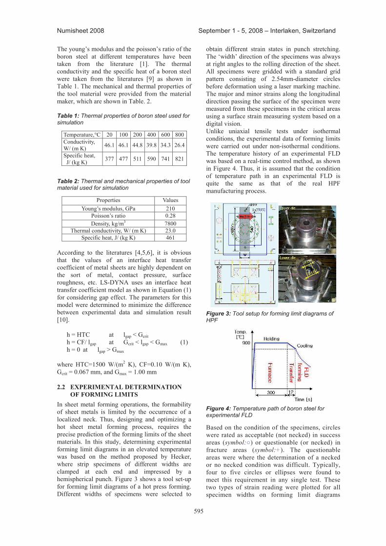
595


The young’s modulus and the poisson’s ratio of the boron steel at different temperatures have been taken from the literature [1]. The thermal conductivity and the specific heat of a boron steel were taken from the literatures [9] as shown in Table 1. The mechanical and thermal properties of the tool material were provided from the material maker, which are shown in Table. 2.

Table 1: Thermal properties of boron steel used for simulation

Temperature,°C 20 100 200 400 600 800Conductivity, W/ (m K) 46.1 46.1 44.8 39.8 34.3 26.4

Specific heat, J/ (kg K) 377 477 511 590 741 821

Table 2: Thermal and mechanical properties of tool material used for simulation

Properties Values Young’s modulus, GPa 210

Poisson’s ratio 0.28 Density, kg/m3 7800

Thermal conductivity, W/ (m K) 23.0 Specific heat, J/ (kg K) 461

According to the literatures [4,5,6], it is obvious that the values of an interface heat transfer coefficient of metal sheets are highly dependent on the sort of metal, contact pressure, surface roughness, etc. LS-DYNA uses an interface heat transfer coefficient model as shown in Equation (1)for considering gap effect. The parameters for this model were determined to minimize the difference between experimental data and simulation result [10].

h = HTC at lgap < Gcrit h = CF/ lgap at Gcrit < lgap < Gmax (1) h = 0 at lgap > Gmax

where HTC=1500 W/(m2 K), CF=0.10 W/(m K), Gcrit = 0.067 mm, and Gmax = 1.00 mm

2.2 eXperIMeNtaL DeterMINatION OF FOrMING LIMItS

In sheet metal forming operations, the formability of sheet metals is limited by the occurrence of a localized neck. Thus, designing and optimizing a hot sheet metal forming process, requires the precise prediction of the forming limits of the sheet materials. In this study, determining experimental forming limit diagrams in an elevated temperature was based on the method proposed by Hecker, where strip specimens of different widths are clamped at each end and impressed by a hemispherical punch. Figure 3 shows a tool set-up for forming limit diagrams of a hot press forming. Different widths of specimens were selected to

obtain different strain states in punch stretching. The ‘width’ direction of the specimens was always at right angles to the rolling direction of the sheet. All specimens were gridded with a standard grid pattern consisting of 2.54mm-diameter circles before deformation using a laser marking machine. The major and minor strains along the longitudinal direction passing the surface of the specimen were measured from these specimens in the critical areas using a surface strain measuring system based on a digital vision. Unlike uniaxial tensile tests under isothermal conditions, the experimental data of forming limits were carried out under non-isothermal conditions. The temperature history of an experimental FLD was based on a real-time control method, as shown in Figure 4. Thus, it is assumed that the condition of temperature path in an experimental FLD is quite the same as that of the real HPF manufacturing process.

Figure 3: Tool setup for forming limit diagrams of HPF

Figure 4: Temperature path of boron steel for experimental FLD

Based on the condition of the specimens, circles were rated as acceptable (not necked) in success areas (symbol:) or questionable (or necked) in fracture areas (symbol:+). The questionable areas were where the determination of a necked or no necked condition was difficult. Typically, four to five circles or ellipses were found to meet this requirement in any single test. These two types of strain reading were plotted for all specimen widths on forming limit diagrams

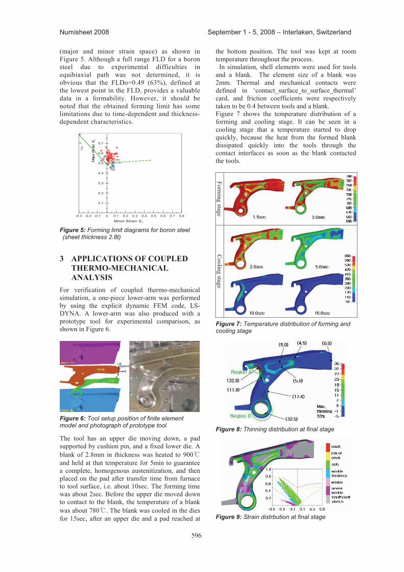
596


(major and minor strain space) as shown in Figure 5. Although a full range FLD for a boron steel due to experimental difficulties in equibiaxial path was not determined, it is obvious that the FLDo=0.49 (63%), defined at the lowest point in the FLD, provides a valuable data in a formability. However, it should be noted that the obtained forming limit has some limitations due to time-dependent and thickness-dependent characteristics.

-0.3 -0.2 -0.1 0 0.1 0.2 0.3 0.4 0.5 0.6 0.7 0.8

Minor Strain ε2

0.1

0.2

0.3

0.4

0.5

0.6

0.7

M

ajor

Stra

in ε

1

Figure 5: Forming limit diagrams for boron steel (sheet thickness 2.8t)

3 appLICatIONS OF COUpLeD therMO-MeChaNICaL aNaLYSIS

For verification of coupled thermo-mechanical simulation, a one-piece lower-arm was performed by using the explicit dynamic FEM code, LS-DYNA. A lower-arm was also produced with a prototype tool for experimental comparison, as shown in Figure 6.

Figure 6: Tool setup position of finite element model and photograph of prototype tool

The tool has an upper die moving down, a pad supported by cushion pin, and a fixed lower die. A blank of 2.8mm in thickness was heated to 900and held at that temperature for 5min to guarantee a complete, homogenous austenitization, and then placed on the pad after transfer time from furnace to tool surface, i.e. about 10sec. The forming time was about 2sec. Before the upper die moved down to contact to the blank, the temperature of a blankwas about 780 . The blank was cooled in the dies for 15sec, after an upper die and a pad reached at

the bottom position. The tool was kept at room temperature throughout the process.

In simulation, shell elements were used for tools and a blank. The element size of a blank was 2mm. Thermal and mechanical contacts were defined in ‘contact_surface_to_surface_thermal’ card, and friction coefficients were respectively taken to be 0.4 between tools and a blank. Figure 7 shows the temperature distribution of a forming and cooling stage. It can be seen in a cooling stage that a temperature started to drop quickly, because the heat from the formed blank dissipated quickly into the tools through the contact interfaces as soon as the blank contacted the tools.

Forming stage

Cooling stage

Figure 7: Temperature distribution of forming and cooling stage

Figure 8: Thinning distribution at final stage

Figure 9: Strain distrbution at final stage

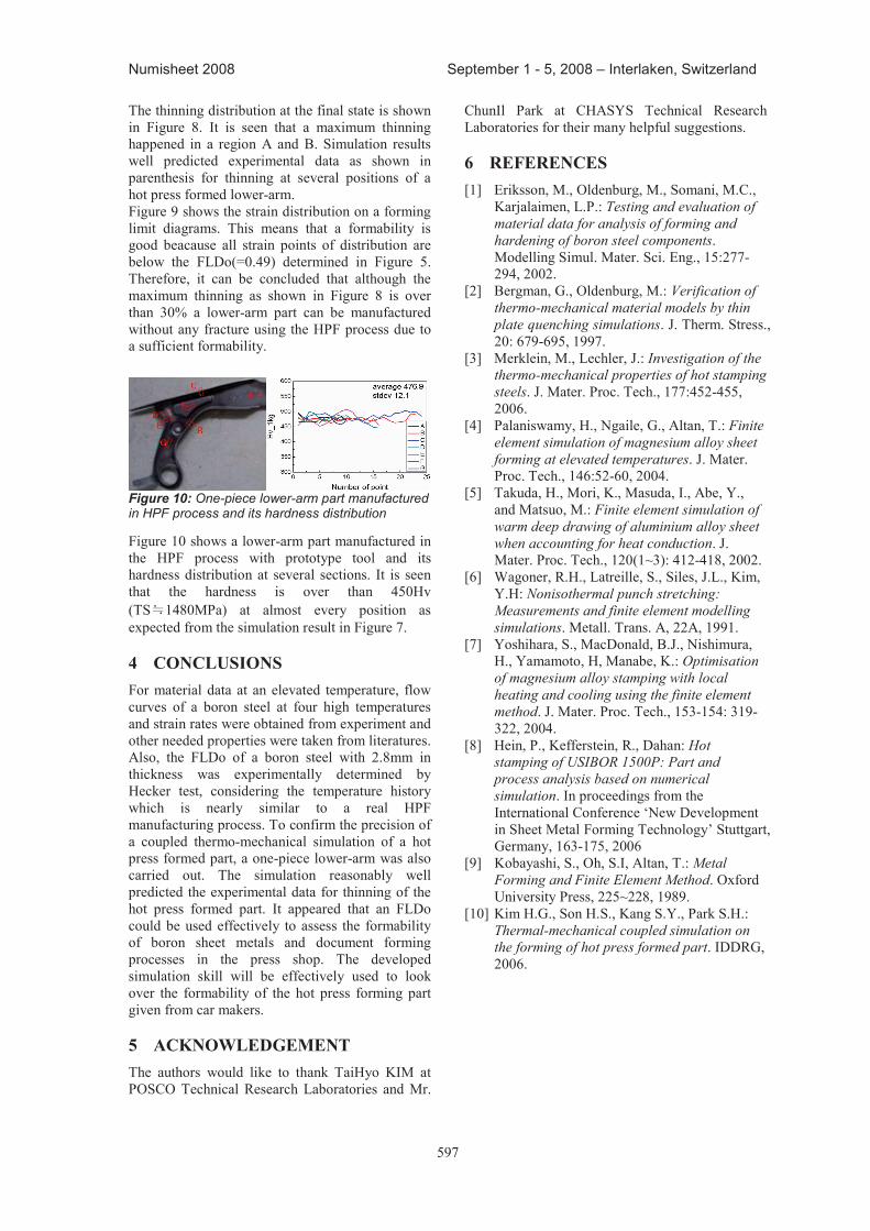
597


The thinning distribution at the final state is shown in Figure 8. It is seen that a maximum thinning happened in a region A and B. Simulation results well predicted experimental data as shown in parenthesis for thinning at several positions of a hot press formed lower-arm. Figure 9 shows the strain distribution on a forming limit diagrams. This means that a formability is good beacause all strain points of distribution arebelow the FLDo(=0.49) determined in Figure 5. Therefore, it can be concluded that although the maximum thinning as shown in Figure 8 is over than 30% a lower-arm part can be manufactured without any fracture using the HPF process due to a sufficient formability.

Figure 10: One-piece lower-arm part manufactured in HPF process and its hardness distribution

Figure 10 shows a lower-arm part manufactured in the HPF process with prototype tool and its hardness distribution at several sections. It is seen that the hardness is over than 450Hv (TS 1480MPa) at almost every position as expected from the simulation result in Figure 7.

4 CONCLUSIONS For material data at an elevated temperature, flow curves of a boron steel at four high temperatures and strain rates were obtained from experiment and other needed properties were taken from literatures. Also, the FLDo of a boron steel with 2.8mm in thickness was experimentally determined by Hecker test, considering the temperature history which is nearly similar to a real HPF manufacturing process. To confirm the precision of a coupled thermo-mechanical simulation of a hot press formed part, a one-piece lower-arm was also carried out. The simulation reasonably well predicted the experimental data for thinning of the hot press formed part. It appeared that an FLDo could be used effectively to assess the formability of boron sheet metals and document forming processes in the press shop. The developed simulation skill will be effectively used to look over the formability of the hot press forming part given from car makers.

5 aCKNOWLeDGeMeNt The authors would like to thank TaiHyo KIM at POSCO Technical Research Laboratories and Mr.

ChunIl Park at CHASYS Technical Research Laboratories for their many helpful suggestions.

6 reFereNCeS [1] Eriksson, M., Oldenburg, M., Somani, M.C.,

Karjalaimen, L.P.: Testing and evaluation of material data for analysis of forming and hardening of boron steel components. Modelling Simul. Mater. Sci. Eng., 15:277-294, 2002.

[2] Bergman, G., Oldenburg, M.: Verification of thermo-mechanical material models by thin plate quenching simulations. J. Therm. Stress., 20: 679-695, 1997.

[3] Merklein, M., Lechler, J.: Investigation of the thermo-mechanical properties of hot stamping steels. J. Mater. Proc. Tech., 177:452-455, 2006.

[4] Palaniswamy, H., Ngaile, G., Altan, T.: Finite element simulation of magnesium alloy sheet forming at elevated temperatures. J. Mater. Proc. Tech., 146:52-60, 2004.

[5] Takuda, H., Mori, K., Masuda, I., Abe, Y., and Matsuo, M.: Finite element simulation of warm deep drawing of aluminium alloy sheet when accounting for heat conduction. J. Mater. Proc. Tech., 120(1~3): 412-418, 2002.

[6] Wagoner, R.H., Latreille, S., Siles, J.L., Kim, Y.H: Nonisothermal punch stretching: Measurements and finite element modelling simulations. Metall. Trans. A, 22A, 1991.

[7] Yoshihara, S., MacDonald, B.J., Nishimura, H., Yamamoto, H, Manabe, K.: Optimisation of magnesium alloy stamping with local heating and cooling using the finite element method. J. Mater. Proc. Tech., 153-154: 319-322, 2004.

[8] Hein, P., Kefferstein, R., Dahan: Hot stamping of USIBOR 1500P: Part and process analysis based on numerical simulation. In proceedings from the International Conference ‘New Development in Sheet Metal Forming Technology’ Stuttgart, Germany, 163-175, 2006

[9] Kobayashi, S., Oh, S.I, Altan, T.: Metal Forming and Finite Element Method. Oxford University Press, 225~228, 1989.

[10] Kim H.G., Son H.S., Kang S.Y., Park S.H.: Thermal-mechanical coupled simulation on the forming of hot press formed part. IDDRG, 2006.

599


____________________* Corresponding author: School of Mechanical Engineering, Shanghai Jiaotong University, Shanghai, 200240, China, +86-21-34206312, +86-21-34206312, [email protected]

NUMerICaL SIMULatION OF WarM StaMpING OF aZ31 MaGNeSIUM aLLOY Sheet BaSeD ON therMO-

MeChaNICaL COUpLeD MethOD

Ying-hong peNG, Qun-Feng ChaNG*, Da-Yong LI,

School of Mechanical Engineering, Shanghai Jiaotong University, Shanghai, 200240, China

aBStraCt: In this study, uni-axial tension experiments of a cross-rolled AZ31 sheet are conducted using Gleeble 3500 thermal - mechanical simulator under different temperature and strain rate conditions. Mechanical propriety of AZ31 magnesium alloy sheet is analyzed according to the true strain-stress curves. The flow stress-strain relation is introduced into the commercial finite element software LS-DYNA as the material constitutive model. Then the thermo-mechanical coupled simulation of the warm stamping process of AZ31 magnesium alloy sheets is performed with LS-DYNA. Heat conduction between stamping tools is calculated. The deformation behaviour and the temperature change in the drawing process are investigated. Due to the heat conduction, there is non-uniform distribution of temperature along flange area, force transfer area and deformation area. Therefore the resistance of the force transfer area is enhanced and the warm formability of magnesium alloy sheet can be further improved. The thermo-mechanical coupled simulation provides a good guide for the development of non-isothermal drawing techniques.

KeYWOrDS: AZ31 magnesium alloy sheet; warm stamping; numerical simulation; thermo-mechanical coupled.

1 INtrODUCtIONDue to its high specific strength, high productivity and low manufacturing cost, sheet metal forming production of magnesium alloy offers great potential for growth in the automotive and 3C industry. Although casting is still the dominant method in manufacturing of magnesium alloy components, plastic forming technology of magnesium alloys has been paid more and more attention since forming products exhibit better quality than casting ones[1, 2].Because of the close-packed crystal structure of magnesium, the stamping of magnesium alloy sheet is difficult under room temperature. The ductility of the magnesium alloy can improve with increase in the working temperature, which makes warm stamping one important way to obtain good formability for magnesium alloy sheets. In order to find the optimal process parameters for warm stamping of the magnesium alloy sheets, it is necessary to study not only the mechanical properties of magnesium alloy sheets under different temperature but also the process conditions during forming.

Quite a few efforts have been made to study the warm forming of magnesium alloy sheet with experimental and simulation method[3, 9]. Takuda examined the formability of AZ31 magnesium alloy sheet by the finite element method and the forming limit is predicted. Doege conducted drawing tests with magnesium alloys in temperature range between 200~250 C, and investigated the influence of forming speed on limit drawing ratio. Yoshihara studied the influence of blank holder force on the forming of magnesium alloy sheet. Palaniswamy simulated forming processes of round cups and rectangular pans from magnesium alloy at elevated temperatures. Zhang conducted tests on deep drawing of magnesium alloy sheet and obtained a limit drawing ratio up to 2.6 at 170 C. In the present paper, a non-thermal drawing process of magnesium alloy sheet is numerical studied by the thermo-mechanical finite element method. Temperature and stress distribution in the drawing process are investigated and the influence of heat conduction on formability improvement of warm drawing is discussed.

600


2 MeChaNICaL prOprIetY Uniaxial tensile tests are performed to obtain the mechanical properties of magnesium alloy sheet at widely range of strain rates and temperatures. The processing parameters of uniaxial tensile tests are listed in Tab. 1.

Table 1: Processing parameters of uniaxial tensile tests

Strain rate (S-1) 0.002, 0.02 ，0.2，2

Drawing temperature (℃) RT,100,150,200,250

Sample length (mm) 15

Sample width (mm) 10

Sample thickness (mm) 0.6

Elongations under various test temperatures at the strain rate of 0.02 )( 1s are shown in Fig. 1. It is found in Fig. 1 that the elongation is 18% at room temperature, and obviously increases as the test temperature increases. When the temperature is above 200℃, the elongation is higher than 50%,

and it reach 100% at the temperature of 400℃. It is evident that the magnesium alloy sheet shows good ductility when the temperature is above 200℃.

Figure 1: Elongation at various temperatures

The true stress-strain curves corresponding to different temperatures and strain rates obtained from the tensile tests are shown in Fig. 2. Fig. 2 (a) shows the influence of strain rates on the flow stress at the temperature of 200 ℃ . It is demonstrated that the ductility of AZ31 magnesium alloy sheet rises significantly with the decrease of strain rate, exhibiting obvious strain rate sensitivity. Fig. 2 (b) shows the influence of

test temperatures on the flow stress at the strain rate of 0.02 )( 1s . It can be seen that the yield stress and tensile strength are sharply decrease as the test temperature increases. When the temperature is above 250℃ , due to dynamic recovery, no obvious work hardening is observed.

Figure 2: True stress-strain curves under different processing parameters

(a) T=200℃ (b) 2102

3 FINIte eLeMeNt MODeL OF therMaL-MeChaNICaLSeQUeNCe COUpLeD

The function of temperature field can be expressed by ),,( tZRT in cylindrical coordinates. The differential equation of transient heat conduction can be expressed as:

tTcq

ZT

RT

RRT )1( 2

2

2

2

(1)

Where is the thermal conductivity, T is the temperature, c is the specific heat, is the

density, q is the heat generation rate.

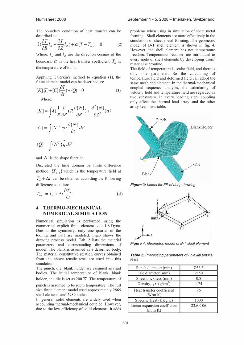
601


The boundary condition of heat transfer can be described as:

0)()( TTlZTl

RT

ZR (2)

Where: Rl and Zl are the direction cosines of the

boundary, is the heat transfer coefficient, T is the temperature of tools.

Applying Galerkin’s method to equation (1), the finite element model can be described as:

0}{}]{[}]{[ QtTCTK (3)

Where:

V

dVZ

NRNR

RRK )}{)}{(1(][ 2

2

V

T dVtNcNC }{}{][

V

T dVqNQ }{}{

and N is the shape function.

Discreted the time domain by finite difference method, }{ 1nT which is the temperature field at

tTn can be obtained according the following difference equation:

tT

tTT nnn 1 (4)

4 therMO-MeChaNICaL NUMerICaL SIMULatION

Numerical simulation is performed using the commercial explicit finite element code LS-Dyna. Due to the symmetry, only one quarter of the tooling and part are modeled. Fig.3 shows the drawing process model. Tab. 2 lists the material parameters and corresponding dimensions of model. The blank is assumed as a deformed body. The material constitutive relation curves obtained from the above tensile tests are used into this simulation. The punch, die, blank holder are assumed as rigid bodies. The initial temperature of blank, blank holder, and die is set as 200 ℃. The temperature of punch is assumed to be room temperature. The full size finite element model used approximately 2665 shell elements and 2989 nodes. In general, solid elements are widely used when accounting thermal-mechanical coupled. However, due to the low efficiency of solid elements, it adds

problems when using in simulation of sheet metal forming. Shell elements are more effectively in the simulation of sheet metal forming. The geometric model of B-T shell element is shown in fig. 4. However, the shell element has not temperature freedom. Temperature freedoms are introduced to every node of shell elements by developing users’ material subroutine. The field of temperature is scalar field, and there is only one parameter. So the calculating of temperature field and deformed field can adopt the same mesh and element. In the thermal-mechanical coupled sequence analysis, the calculating of velocity field and temperature field are regarded as two subsystem. In every loading step, coupling only affect the thermal load array, and the other array keep invariable.

Figure 3: Model for FE of deep drawing

Figure 4: Geometric model of B-T shell element

Table 2: Processing parameters of uniaxial tensile tests

Punch diameter (mm) Ø53.5 Die diameter (mm) Ø 50

Sheet thickness (mm) 0.8 Density, (g/cm3) 1.74

Heat transfer coefficient (W/m K)

96

Specific Heat (J/Kg K) 1000 Linear expansion coefficient

(m/m K) 23.6E-06

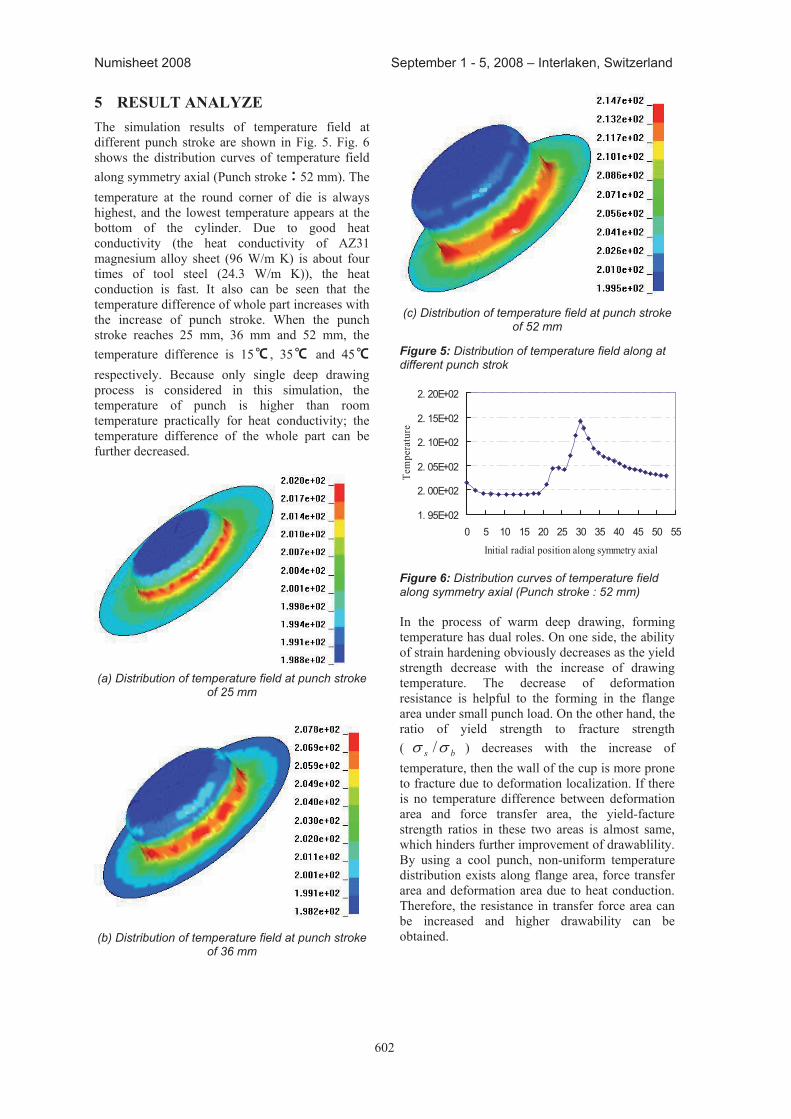
602


5 reSULt aNaLYZe The simulation results of temperature field at different punch stroke are shown in Fig. 5. Fig. 6 shows the distribution curves of temperature field along symmetry axial (Punch stroke：52 mm). The temperature at the round corner of die is always highest, and the lowest temperature appears at the bottom of the cylinder. Due to good heat conductivity (the heat conductivity of AZ31 magnesium alloy sheet (96 W/m K) is about four times of tool steel (24.3 W/m K)), the heat conduction is fast. It also can be seen that the temperature difference of whole part increases with the increase of punch stroke. When the punch stroke reaches 25 mm, 36 mm and 52 mm, the temperature difference is 15℃ , 35℃ and 45℃respectively. Because only single deep drawing process is considered in this simulation, the temperature of punch is higher than room temperature practically for heat conductivity; the temperature difference of the whole part can be further decreased.

(a) Distribution of temperature field at punch stroke of 25 mm

(b) Distribution of temperature field at punch stroke of 36 mm

(c) Distribution of temperature field at punch stroke of 52 mm

Figure 5: Distribution of temperature field along at different punch strok

1. 95E+02

2. 00E+02

2. 05E+02

2. 10E+02

2. 15E+02

2. 20E+02

0 5 10 15 20 25 30 35 40 45 50 55

Initial radial position along symmetry axial

Tem

pera

ture

Figure 6: Distribution curves of temperature field along symmetry axial (Punch stroke : 52 mm)

In the process of warm deep drawing, forming temperature has dual roles. On one side, the ability of strain hardening obviously decreases as the yield strength decrease with the increase of drawing temperature. The decrease of deformation resistance is helpful to the forming in the flange area under small punch load. On the other hand, the ratio of yield strength to fracture strength ( bs / ) decreases with the increase of temperature, then the wall of the cup is more prone to fracture due to deformation localization. If there is no temperature difference between deformation area and force transfer area, the yield-facture strength ratios in these two areas is almost same, which hinders further improvement of drawablility. By using a cool punch, non-uniform temperature distribution exists along flange area, force transfer area and deformation area due to heat conduction. Therefore, the resistance in transfer force area can be increased and higher drawability can be obtained.

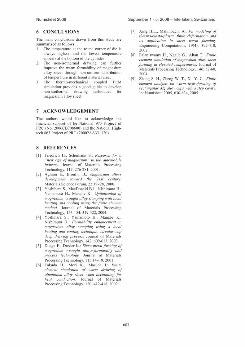
603


6 CONCLUSIONS The main conclusions drawn from this study are summarized as follows. 1. The temperature at the round corner of die is

always highest, and the lowest temperature appears at the bottom of the cylinder

2. The non-isothermal drawing can further improve the warm formability of magnesium alloy sheet through non-uniform distribution of temperature in different material area;

3. The thermo-mechanical coupled FEM simulation provides a good guide to develop non-isothermal drawing techniques for magnesium alloy sheet.

7 aCKNOWLeDGeMeNt The authors would like to acknowledge the financial support of he National 973 Project of PRC (No. 2006CB708600) and the National High-tech 863 Project of PRC (20002AA331120).

8 reFereNCeS [1] Friedrich H., Schumann S.: Research for a

“new age of magnesium” in the automobile industry. Journal of Materials Processing Technology, 117: 276-281, 2001.

[2] Aghion E., Bronfin B.: Magnesium alloys development toward the 21st century. Materials Science Forum, 22:19 28, 2000.

[3] Yoshihara S., MacDonald B.J., Nishimura H., Yamamoto H., Manabe K.: Optimization of magnesium wrought alloy stamping with local heating and cooling using the finite element method. Journal of Materials Processing Technology, 153-154: 319-322, 2004.

[4] Yoshihara S., Yamamoto H., Manabe K., Nishimura H.: Formability enhancement in magnesium alloy stamping using a local heating and cooling technique: circular cup deep drawing process. Journal of Materials Processing Technology, 142: 609-613, 2003.

[5] Doege E., Droder K.: Sheet metal forming of magnesium wrought alloys-formability and process technology. Journal of Materials Processing Technology, 115:14 19, 2001.

[6] Takuda H., Mori K., Masuda I.: Finite element simulation of warm drawing of aluminium alloy sheet when accounting for heat conduction. Journal of Materials Processing Technology, 120: 412-418, 2002.

[7] Xing H.L., Makinouchi A.: FE modeling of thermo-elasto-plastic finite deformation and its application in sheet warm forming.Engineering Computations, 19(4): 392-410, 2002.

[8] Palaniswamy H., Ngaile G., Altan T.: Finite element simulation of magnesium alloy sheet forming at elevated temperatures. Journal of Materials Processing Technology, 146: 52-60, 2004,.

[9] Zhang S. H., Zheng W. T., Xu Y. C.: Finite element analysis on warm hydroforming of rectangular Mg alloy cups with a step cavity.In: Numisheet 2005, 630-634, 2005.

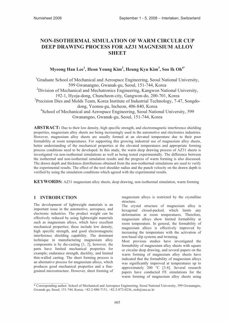
605


____________________ * Corresponding author: School of Mechanical and Aerospace Engineering, Seoul National University, 599 Gwanangno, Gwanak-gu, Seoul, 151-744, Korea, +82-2-880-7151, +82-2-872-0236, [email protected]

NON-ISOtherMaL SIMULatION OF WarM CIrCULr CUp Deep DraWING prOCeSS FOr aZ31 MaGNeSIUM aLLOY

Sheet

Myeong han Lee1, heon Young Kim2, heung Kyu Kim3, Soo Ik Oh4*

1Graduate School of Mechanical and Aerospace Engineering, Seoul National University,

599 Gwanangno, Gwanak-gu, Seoul, 151-744, Korea 2Division of Mechanical and Mechatronics Engineering, Kangwon National University,

192-1, Hyoja-dong, Chuncheon-city, Gangwon-do, 200-701, Korea 3Precision Dies and Molds Team, Korea Institute of Industrial Technology, 7-47, Songdo-

dong, Yeonsu-gu, Incheon, 406-840, Korea 4School of Mechanical and Aerospace Engineering, Seoul National University, 599

Gwanangno, Gwanak-gu, Seoul, 151-744, Korea aBStraCt: Due to their low density, high specific strength, and electromagnetic interference shielding properties, magnesium alloy sheets are being increasingly used in the automotive and electronics industries. However, magnesium alloy sheets are usually formed at an elevated temperature due to their poor formability at room temperatures. For supporting this growing industrial use of magnesium alloy sheets, better understanding of the mechanical properties at the elevated temperatures and appropriate forming process conditions need to be developed. In this study, the warm deep drawing process of AZ31 sheets is investigated via non-isothermal simulations as well as being tested experimentally. The difference between the isothermal and non-isothermal simulation results and the progress of warm forming is also discussed. The drawn depth and thickness distributions obtained from the non-isothermal simulations are used to verify the experimental results. The effect of the tool shoulder radius and the punch velocity on the drawn depth is verified by using the simulation conditions which agreed with the experimental results.

KeYWOrDS: AZ31 magnesium alloy sheets, deep drawing, non-isothermal simulation, warm forming 1 INtrODUCtIONThe development of lightweight materials is an important issue in the automotive, aerospace, and electronic industries. The product weight can be effectively reduced by using lightweight materials such as magnesium alloys, which have excellent mechanical properties; these include low density, high specific strength, and good electromagnetic interference shielding capability. The dominant technique in manufacturing magnesium alloy components is by die-casting [1, 2], however, the parts have limited mechanical properties for example; endurance strength, ductility, and limited thin-walled casting. The sheet forming process is an alternative process for magnesium alloys, which produces good mechanical properties and a fine-grained microstructure. However, sheet forming of

magnesium alloys is restricted by the crystalline structure. The crystal structure of magnesium alloy is hexagonal closed-packed, which limits any deformation at room temperatures. Therefore, magnesium alloys show limited formability at room temperature. In general, the formability of magnesium alloys is effectively improved by increasing the temperature with the activation of non-basal slip systems and twinning. Most previous studies have investigated the formability of magnesium alloy sheets with square or circular deep drawing, and several papers on the warm forming of magnesium alloy sheets have indicated that the formability of magnesium alloys was significantly improved at temperatures up to approximately 200 °C [3-8]. Several research papers have conducted FE simulations for the warm forming of magnesium alloy sheets using

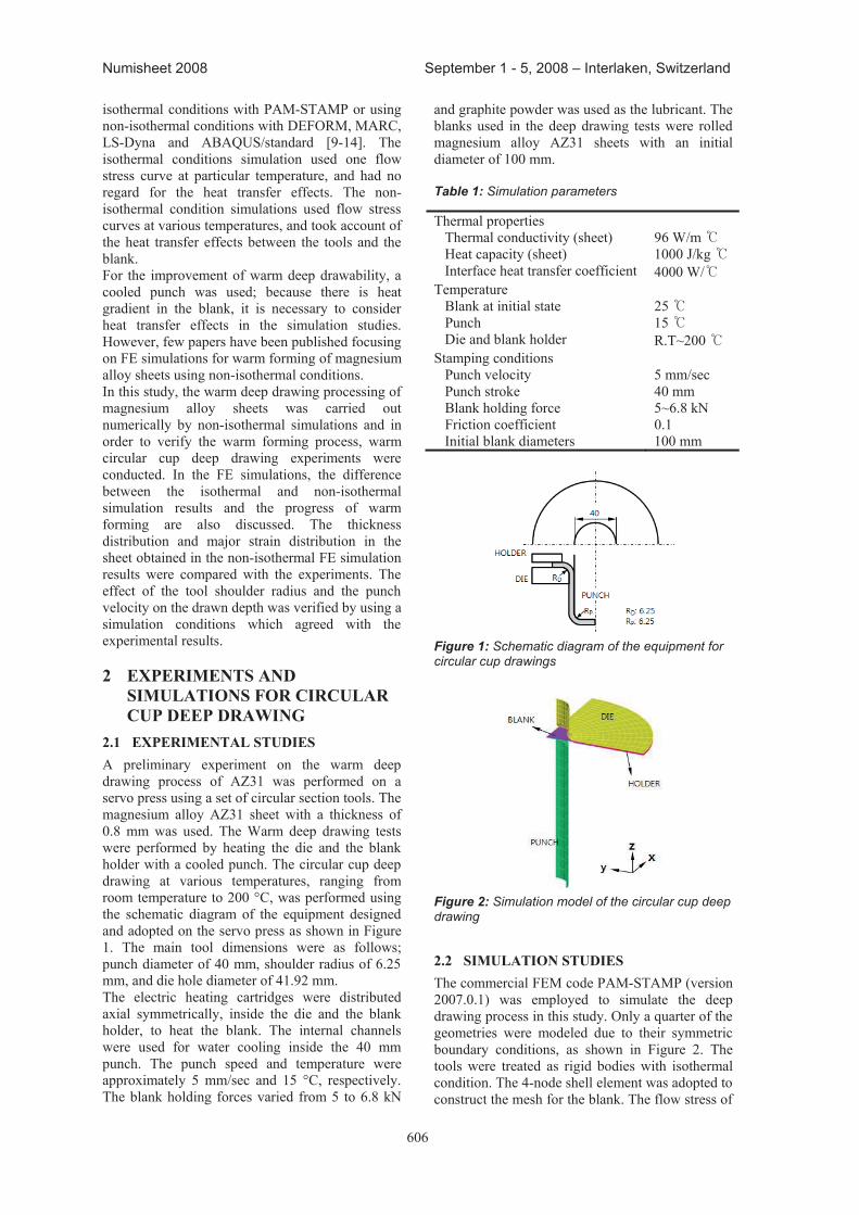
606


isothermal conditions with PAM-STAMP or using non-isothermal conditions with DEFORM, MARC, LS-Dyna and ABAQUS/standard [9-14]. The isothermal conditions simulation used one flow stress curve at particular temperature, and had no regard for the heat transfer effects. The non-isothermal condition simulations used flow stress curves at various temperatures, and took account of the heat transfer effects between the tools and the blank. For the improvement of warm deep drawability, a cooled punch was used; because there is heat gradient in the blank, it is necessary to consider heat transfer effects in the simulation studies. However, few papers have been published focusing on FE simulations for warm forming of magnesium alloy sheets using non-isothermal conditions. In this study, the warm deep drawing processing of magnesium alloy sheets was carried out numerically by non-isothermal simulations and in order to verify the warm forming process, warm circular cup deep drawing experiments were conducted. In the FE simulations, the difference between the isothermal and non-isothermal simulation results and the progress of warm forming are also discussed. The thickness distribution and major strain distribution in the sheet obtained in the non-isothermal FE simulation results were compared with the experiments. The effect of the tool shoulder radius and the punch velocity on the drawn depth was verified by using a simulation conditions which agreed with the experimental results. 2 eXperIMeNtS aND

SIMULatIONS FOr CIrCULar CUp Deep DraWING

2.1 eXperIMeNtaL StUDIeS A preliminary experiment on the warm deep drawing process of AZ31 was performed on a servo press using a set of circular section tools. The magnesium alloy AZ31 sheet with a thickness of 0.8 mm was used. The Warm deep drawing tests were performed by heating the die and the blank holder with a cooled punch. The circular cup deep drawing at various temperatures, ranging from room temperature to 200 °C, was performed using the schematic diagram of the equipment designed and adopted on the servo press as shown in Figure 1. The main tool dimensions were as follows; punch diameter of 40 mm, shoulder radius of 6.25 mm, and die hole diameter of 41.92 mm. The electric heating cartridges were distributed axial symmetrically, inside the die and the blank holder, to heat the blank. The internal channels were used for water cooling inside the 40 mm punch. The punch speed and temperature were approximately 5 mm/sec and 15 °C, respectively. The blank holding forces varied from 5 to 6.8 kN

and graphite powder was used as the lubricant. The blanks used in the deep drawing tests were rolled magnesium alloy AZ31 sheets with an initial diameter of 100 mm. Table 1: Simulation parameters

Thermal properties Thermal conductivity (sheet) 96 W/m Heat capacity (sheet) 1000 J/kg Interface heat transfer coefficient 4000 W/ Temperature Blank at initial state 25 Punch 15 Die and blank holder R.T~200 Stamping conditions Punch velocity 5 mm/sec Punch stroke 40 mm Blank holding force 5~6.8 kN Friction coefficient 0.1 Initial blank diameters 100 mm

Figure 1: Schematic diagram of the equipment for circular cup drawings

Figure 2: Simulation model of the circular cup deep drawing

2.2 SIMULatION StUDIeS The commercial FEM code PAM-STAMP (version 2007.0.1) was employed to simulate the deep drawing process in this study. Only a quarter of the geometries were modeled due to their symmetric boundary conditions, as shown in Figure 2. The tools were treated as rigid bodies with isothermal condition. The 4-node shell element was adopted to construct the mesh for the blank. The flow stress of

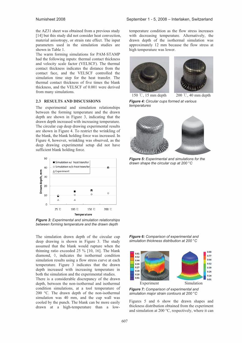
607


the AZ31 sheet was obtained from a previous study [14] but this study did not consider heat convection, material anisotropy, or strain rate effect. The input parameters used in the simulation studies are shown in Table 1. The warm forming simulations for PAM-STAMP had the following inputs: thermal contact thickness and velocity scale factor (VELSCF). The thermal contact thickness indicates the distance from the contact face, and the VELSCF controlled the simulation time step for the heat transfer. The thermal contact thickness of five times the blank thickness, and the VELSCF of 0.001 were derived from many simulations. 2.3 reSULtS aND DISCUSSIONS The experimental and simulation relationships between the forming temperature and the drawn depth are shown in Figure 3, indicating that the drawn depth increased with increasing temperature. The circular cup deep drawing experimental results are shown in Figure 4. To restrict the wrinkling of the blank, the blank holding force was increased. In Figure 4, however, wrinkling was observed, as the deep drawing experimental setup did not have sufficient blank holding force.

Figure 3: Experimental and simulation relationships between forming temperature and the drawn depth

The simulation drawn depth of the circular cup deep drawing is shown in Figure 3. The study assumed that the blank would rupture when the thinning ratio exceeded 25 % [10, 16]. The blank diamond, ◊, indicates the isothermal condition simulation results using a flow stress curve at each temperature. Figure 3 indicates that the drawn depth increased with increasing temperature in both the simulation and the experimental studies. There is a considerable discrepancy of the drawn depth, between the non-isothermal and isothermal condition simulations, at a tool temperature of 200 °C. The drawn depth of the non-isothermal simulation was 40 mm, and the cup wall was cooled by the punch. The blank can be more easily drawn at a high-temperature than a low-

temperature condition as the flow stress increases with decreasing temperature. Alternatively, the drawn depth of the isothermal simulation was approximately 12 mm because the flow stress at high temperature was lower.

150 , 15 mm depth 200 , 40 mm depth Figure 4: Circular cups formed at various temperatures

Figure 5: Experimental and simulations for the drawn shape the circular cup at 200 °C

Figure 6: Comparison of experimental and simulation thickness distribution at 200 °C

Experiment Simulation Figure 7: Comparison of experimental and simulation major strain contours at 200 °C

Figures 5 and 6 show the drawn shapes and thickness distribution obtained from the experiment and simulation at 200 °C, respectively, where it can

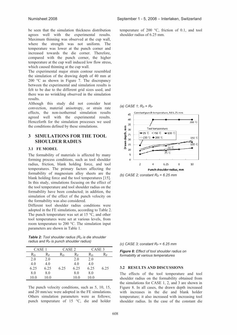
608


be seen that the simulation thickness distribution agrees well with the experimental results. Maximum thinning was observed at the cup wall, where the strength was not uniform. The temperature was lower at the punch corner and increased towards the die corner. Therefore, compared with the punch corner, the higher temperature at the cup wall induced low flow stress, which caused thinning at the cup wall. The experimental major strain contour resembled the simulation of the drawing depth of 40 mm at 200 °C as shown in Figure 7. The discrepancy between the experimental and simulation results is felt to be due to the different grid sizes used, and there was no wrinkling observed in the simulation results. Although this study did not consider heat convection, material anisotropy, or strain rate effects, the non-isothermal simulation results agreed well with the experimental results. Henceforth for the simulation processes we used the conditions defined by these simulations. 3 SIMULatIONS FOr the tOOL

ShOULDer raDIUS 3.1 Fe MODeL The formability of materials is affected by many forming process conditions, such as tool shoulder radius, friction, blank holding force, and tool temperatures. The primary factors affecting the formability of magnesium alloy sheets are the blank holding force and the tool temperatures [15]. In this study, simulations focusing on the effect of the tool temperature and tool shoulder radius on the formability have been conducted; in addition, the simulation of the effect of the punch velocity on the formability was also considered. Different tool shoulder radius conditions were adopted in the FE simulations, according to Table 2. The punch temperature was set at 15 °C, and other tool temperatures were set at various levels, from room temperature to 200 °C. The simulation input parameters are shown in Table 1. Table 2: Tool shoulder radius (RD is die shoulder radius and RP is punch shoulder radius)

CASE 1 CASE 2 CASE 3 RD RP RD RP RD RP 2.0 2.0

6.25

2.0 2.0

6.25 4.0 4.0 4.0 4.0

6.25 6.25 6.25 6.25 8.0 8.0 8.0 8.0

10.0 10.0 10.0 10.0 The punch velocity conditions, such as 5, 10, 15, and 20 mm/sec were adopted in the FE simulations. Others simulation parameters were as follows; punch temperature of 15 °C, die and holder

temperature of 200 °C, friction of 0.1, and tool shoulder radius of 6.25 mm.

(a) CASE 1; RD = RP

(b) CASE 2; constant RD = 6.25 mm

(c) CASE 3; constant RP = 6.25 mm

Figure 8: Effect of tool shoulder radius on formability at various temperatures

3.2 reSULtS aND DISCUSSIONS The effects of the tool temperature and tool shoulder radius on the formability obtained from the simulations for CASE 1, 2, and 3 are shown in Figure 8. In all cases, the drawn depth increased with increases in the die and blank holder temperature; it also increased with increasing tool shoulder radius. In the case of the constant die

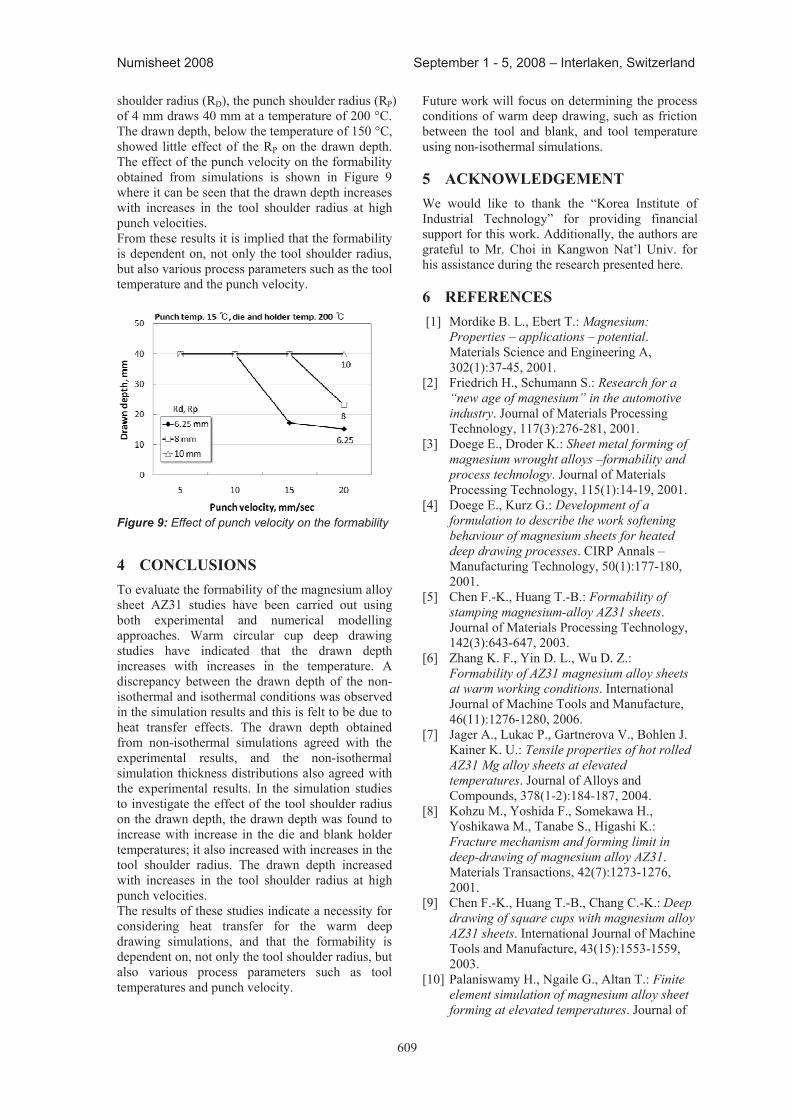
609


shoulder radius (RD), the punch shoulder radius (RP) of 4 mm draws 40 mm at a temperature of 200 °C. The drawn depth, below the temperature of 150 °C, showed little effect of the RP on the drawn depth. The effect of the punch velocity on the formability obtained from simulations is shown in Figure 9 where it can be seen that the drawn depth increases with increases in the tool shoulder radius at high punch velocities. From these results it is implied that the formability is dependent on, not only the tool shoulder radius, but also various process parameters such as the tool temperature and the punch velocity.

Figure 9: Effect of punch velocity on the formability

4 CONCLUSIONS To evaluate the formability of the magnesium alloy sheet AZ31 studies have been carried out using both experimental and numerical modelling approaches. Warm circular cup deep drawing studies have indicated that the drawn depth increases with increases in the temperature. A discrepancy between the drawn depth of the non-isothermal and isothermal conditions was observed in the simulation results and this is felt to be due to heat transfer effects. The drawn depth obtained from non-isothermal simulations agreed with the experimental results, and the non-isothermal simulation thickness distributions also agreed with the experimental results. In the simulation studies to investigate the effect of the tool shoulder radius on the drawn depth, the drawn depth was found to increase with increase in the die and blank holder temperatures; it also increased with increases in the tool shoulder radius. The drawn depth increased with increases in the tool shoulder radius at high punch velocities. The results of these studies indicate a necessity for considering heat transfer for the warm deep drawing simulations, and that the formability is dependent on, not only the tool shoulder radius, but also various process parameters such as tool temperatures and punch velocity.

Future work will focus on determining the process conditions of warm deep drawing, such as friction between the tool and blank, and tool temperature using non-isothermal simulations. 5 aCKNOWLeDGeMeNt We would like to thank the “Korea Institute of Industrial Technology” for providing financial support for this work. Additionally, the authors are grateful to Mr. Choi in Kangwon Nat’l Univ. for his assistance during the research presented here. 6 reFereNCeS [1] Mordike B. L., Ebert T.: Magnesium:

Properties – applications – potential. Materials Science and Engineering A, 302(1):37-45, 2001.

[2] Friedrich H., Schumann S.: Research for a “new age of magnesium” in the automotive industry. Journal of Materials Processing Technology, 117(3):276-281, 2001.

[3] Doege E., Droder K.: Sheet metal forming of magnesium wrought alloys –formability and process technology. Journal of Materials Processing Technology, 115(1):14-19, 2001.

[4] Doege E., Kurz G.: Development of a formulation to describe the work softening behaviour of magnesium sheets for heated deep drawing processes. CIRP Annals – Manufacturing Technology, 50(1):177-180, 2001.

[5] Chen F.-K., Huang T.-B.: Formability of stamping magnesium-alloy AZ31 sheets. Journal of Materials Processing Technology, 142(3):643-647, 2003.

[6] Zhang K. F., Yin D. L., Wu D. Z.: Formability of AZ31 magnesium alloy sheets at warm working conditions. International Journal of Machine Tools and Manufacture, 46(11):1276-1280, 2006.

[7] Jager A., Lukac P., Gartnerova V., Bohlen J. Kainer K. U.: Tensile properties of hot rolled AZ31 Mg alloy sheets at elevated temperatures. Journal of Alloys and Compounds, 378(1-2):184-187, 2004.

[8] Kohzu M., Yoshida F., Somekawa H., Yoshikawa M., Tanabe S., Higashi K.: Fracture mechanism and forming limit in deep-drawing of magnesium alloy AZ31. Materials Transactions, 42(7):1273-1276, 2001.

[9] Chen F.-K., Huang T.-B., Chang C.-K.: Deep drawing of square cups with magnesium alloy AZ31 sheets. International Journal of Machine Tools and Manufacture, 43(15):1553-1559, 2003.

[10] Palaniswamy H., Ngaile G., Altan T.: Finite element simulation of magnesium alloy sheet forming at elevated temperatures. Journal of

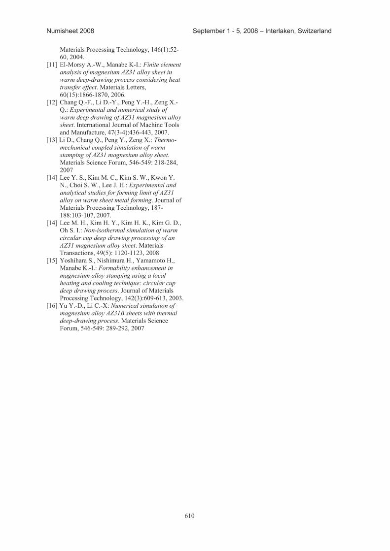
610


Materials Processing Technology, 146(1):52-60, 2004.

[11] El-Morsy A.-W., Manabe K-I.: Finite element analysis of magnesium AZ31 alloy sheet in warm deep-drawing process considering heat transfer effect. Materials Letters, 60(15):1866-1870, 2006.

[12] Chang Q.-F., Li D.-Y., Peng Y.-H., Zeng X.-Q.: Experimental and numerical study of warm deep drawing of AZ31 magnesium alloy sheet. International Journal of Machine Tools and Manufacture, 47(3-4):436-443, 2007.

[13] Li D., Chang Q., Peng Y., Zeng X.: Thermo-mechanical coupled simulation of warm stamping of AZ31 magnesium alloy sheet. Materials Science Forum, 546-549: 218-284, 2007

[14] Lee Y. S., Kim M. C., Kim S. W., Kwon Y. N., Choi S. W., Lee J. H.: Experimental and analytical studies for forming limit of AZ31 alloy on warm sheet metal forming. Journal of Materials Processing Technology, 187-188:103-107, 2007.

[14] Lee M. H., Kim H. Y., Kim H. K., Kim G. D., Oh S. I.: Non-isothermal simulation of warm circular cup deep drawing processing of an AZ31 magnesium alloy sheet. Materials Transactions, 49(5): 1120-1123, 2008

[15] Yoshihara S., Nishimura H., Yamamoto H., Manabe K.-I.: Formability enhancement in magnesium alloy stamping using a local heating and cooling technique: circular cup deep drawing process. Journal of Materials Processing Technology, 142(3):609-613, 2003.

[16] Yu Y.-D., Li C.-X: Numerical simulation of magnesium alloy AZ31B sheets with thermal deep-drawing process. Materials Science Forum, 546-549: 289-292, 2007

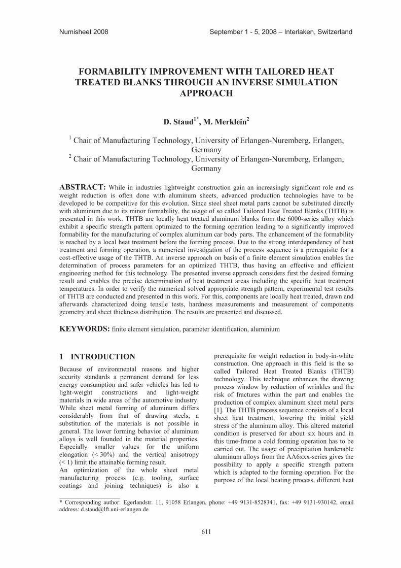
611


____________________ * Corresponding author: Egerlandstr. 11, 91058 Erlangen, phone: +49 9131-8528341, fax: +49 9131-930142, email address: [email protected]

FORMABILITY IMPROVEMENT WITH TAILORED HEAT TREATED BLANKS THROUGH AN INVERSE SIMULATION

APPROACH

D. Staud1*, M. Merklein2

1 Chair of Manufacturing Technology, University of Erlangen-Nuremberg, Erlangen,

Germany 2 Chair of Manufacturing Technology, University of Erlangen-Nuremberg, Erlangen,

Germany ABSTRACT: While in industries lightweight construction gain an increasingly significant role and as weight reduction is often done with aluminum sheets, advanced production technologies have to be developed to be competitive for this evolution. Since steel sheet metal parts cannot be substituted directly with aluminum due to its minor formability, the usage of so called Tailored Heat Treated Blanks (THTB) is presented in this work. THTB are locally heat treated aluminum blanks from the 6000-series alloy which exhibit a specific strength pattern optimized to the forming operation leading to a significantly improved formability for the manufacturing of complex aluminum car body parts. The enhancement of the formability is reached by a local heat treatment before the forming process. Due to the strong interdependency of heat treatment and forming operation, a numerical investigation of the process sequence is a prerequisite for a cost-effective usage of the THTB. An inverse approach on basis of a finite element simulation enables the determination of process parameters for an optimized THTB, thus having an effective and efficient engineering method for this technology. The presented inverse approach considers first the desired forming result and enables the precise determination of heat treatment areas including the specific heat treatment temperatures. In order to verify the numerical solved appropriate strength pattern, experimental test results of THTB are conducted and presented in this work. For this, components are locally heat treated, drawn and afterwards characterized doing tensile tests, hardness measurements and measurement of components geometry and sheet thickness distribution. The results are presented and discussed.

KEYWORDS: finite element simulation, parameter identification, aluminium 1 INTRODUCTION Because of environmental reasons and higher security standards a permanent demand for less energy consumption and safer vehicles has led to light-weight constructions and light-weight materials in wide areas of the automotive industry. While sheet metal forming of aluminum differs considerably from that of drawing steels, a substitution of the materials is not possible in general. The lower forming behavior of aluminum alloys is well founded in the material properties. Especially smaller values for the uniform elongation (< 30%) and the vertical anisotropy (< 1) limit the attainable forming result. An optimization of the whole sheet metal manufacturing process (e.g. tooling, surface coatings and joining techniques) is also a

prerequisite for weight reduction in body-in-white construction. One approach in this field is the so called Tailored Heat Treated Blanks (THTB) technology. This technique enhances the drawing process window by reduction of wrinkles and the risk of fractures within the part and enables the production of complex aluminum sheet metal parts [1]. The THTB process sequence consists of a local sheet heat treatment, lowering the initial yield stress of the aluminum alloy. This altered material condition is preserved for about six hours and in this time-frame a cold forming operation has to be carried out. The usage of precipitation hardenable aluminum alloys from the AA6xxx-series gives the possibility to apply a specific strength pattern which is adapted to the forming operation. For the purpose of the local heating process, different heat

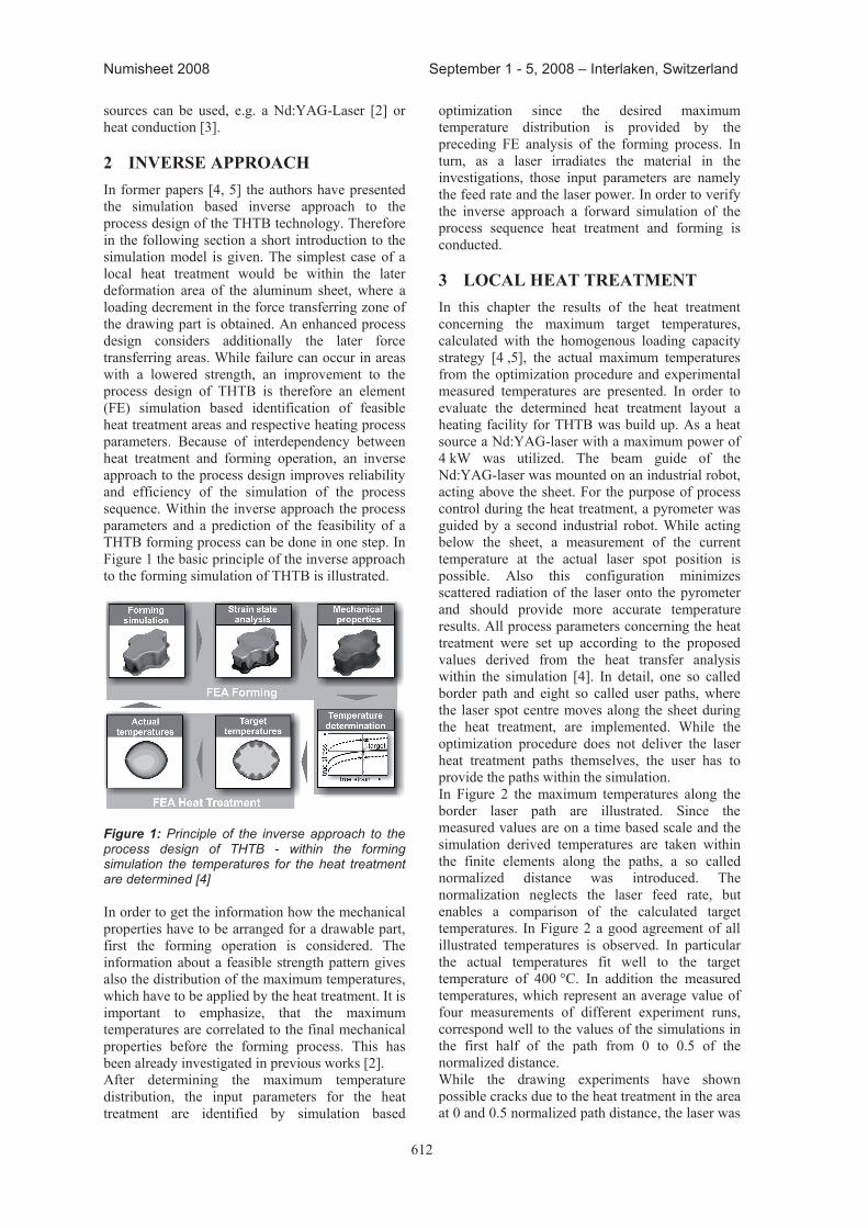
612


sources can be used, e.g. a Nd:YAG-Laser [2] or heat conduction [3]. 2 INVERSE APPROACH In former papers [4, 5] the authors have presented the simulation based inverse approach to the process design of the THTB technology. Therefore in the following section a short introduction to the simulation model is given. The simplest case of a local heat treatment would be within the later deformation area of the aluminum sheet, where a loading decrement in the force transferring zone of the drawing part is obtained. An enhanced process design considers additionally the later force transferring areas. While failure can occur in areas with a lowered strength, an improvement to the process design of THTB is therefore an element (FE) simulation based identification of feasible heat treatment areas and respective heating process parameters. Because of interdependency between heat treatment and forming operation, an inverse approach to the process design improves reliability and efficiency of the simulation of the process sequence. Within the inverse approach the process parameters and a prediction of the feasibility of a THTB forming process can be done in one step. In Figure 1 the basic principle of the inverse approach to the forming simulation of THTB is illustrated.

Figure 1: Principle of the inverse approach to the process design of THTB - within the forming simulation the temperatures for the heat treatment are determined [4] In order to get the information how the mechanical properties have to be arranged for a drawable part, first the forming operation is considered. The information about a feasible strength pattern gives also the distribution of the maximum temperatures, which have to be applied by the heat treatment. It is important to emphasize, that the maximum temperatures are correlated to the final mechanical properties before the forming process. This has been already investigated in previous works [2]. After determining the maximum temperature distribution, the input parameters for the heat treatment are identified by simulation based

optimization since the desired maximum temperature distribution is provided by the preceding FE analysis of the forming process. In turn, as a laser irradiates the material in the investigations, those input parameters are namely the feed rate and the laser power. In order to verify the inverse approach a forward simulation of the process sequence heat treatment and forming is conducted. 3 LOCAL HEAT TREATMENT In this chapter the results of the heat treatment concerning the maximum target temperatures, calculated with the homogenous loading capacity strategy [4 ,5], the actual maximum temperatures from the optimization procedure and experimental measured temperatures are presented. In order to evaluate the determined heat treatment layout a heating facility for THTB was build up. As a heat source a Nd:YAG-laser with a maximum power of 4 kW was utilized. The beam guide of the Nd:YAG-laser was mounted on an industrial robot, acting above the sheet. For the purpose of process control during the heat treatment, a pyrometer was guided by a second industrial robot. While acting below the sheet, a measurement of the current temperature at the actual laser spot position is possible. Also this configuration minimizes scattered radiation of the laser onto the pyrometer and should provide more accurate temperature results. All process parameters concerning the heat treatment were set up according to the proposed values derived from the heat transfer analysis within the simulation [4]. In detail, one so called border path and eight so called user paths, where the laser spot centre moves along the sheet during the heat treatment, are implemented. While the optimization procedure does not deliver the laser heat treatment paths themselves, the user has to provide the paths within the simulation. In Figure 2 the maximum temperatures along the border laser path are illustrated. Since the measured values are on a time based scale and the simulation derived temperatures are taken within the finite elements along the paths, a so called normalized distance was introduced. The normalization neglects the laser feed rate, but enables a comparison of the calculated target temperatures. In Figure 2 a good agreement of all illustrated temperatures is observed. In particular the actual temperatures fit well to the target temperature of 400 °C. In addition the measured temperatures, which represent an average value of four measurements of different experiment runs, correspond well to the values of the simulations in the first half of the path from 0 to 0.5 of the normalized distance. While the drawing experiments have shown possible cracks due to the heat treatment in the area at 0 and 0.5 normalized path distance, the laser was

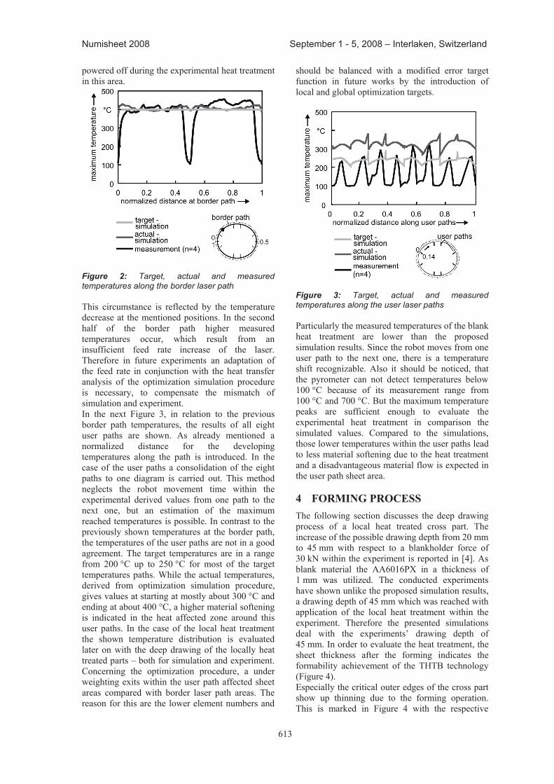
613


powered off during the experimental heat treatment in this area.

Figure 2: Target, actual and measured temperatures along the border laser path This circumstance is reflected by the temperature decrease at the mentioned positions. In the second half of the border path higher measured temperatures occur, which result from an insufficient feed rate increase of the laser. Therefore in future experiments an adaptation of the feed rate in conjunction with the heat transfer analysis of the optimization simulation procedure is necessary, to compensate the mismatch of simulation and experiment. In the next Figure 3, in relation to the previous border path temperatures, the results of all eight user paths are shown. As already mentioned a normalized distance for the developing temperatures along the path is introduced. In the case of the user paths a consolidation of the eight paths to one diagram is carried out. This method neglects the robot movement time within the experimental derived values from one path to the next one, but an estimation of the maximum reached temperatures is possible. In contrast to the previously shown temperatures at the border path, the temperatures of the user paths are not in a good agreement. The target temperatures are in a range from 200 °C up to 250 °C for most of the target temperatures paths. While the actual temperatures, derived from optimization simulation procedure, gives values at starting at mostly about 300 °C and ending at about 400 °C, a higher material softening is indicated in the heat affected zone around this user paths. In the case of the local heat treatment the shown temperature distribution is evaluated later on with the deep drawing of the locally heat treated parts – both for simulation and experiment. Concerning the optimization procedure, a under weighting exits within the user path affected sheet areas compared with border laser path areas. The reason for this are the lower element numbers and

should be balanced with a modified error target function in future works by the introduction of local and global optimization targets.

Figure 3: Target, actual and measured temperatures along the user laser paths Particularly the measured temperatures of the blank heat treatment are lower than the proposed simulation results. Since the robot moves from one user path to the next one, there is a temperature shift recognizable. Also it should be noticed, that the pyrometer can not detect temperatures below 100 °C because of its measurement range from 100 °C and 700 °C. But the maximum temperature peaks are sufficient enough to evaluate the experimental heat treatment in comparison the simulated values. Compared to the simulations, those lower temperatures within the user paths lead to less material softening due to the heat treatment and a disadvantageous material flow is expected in the user path sheet area. 4 FORMING PROCESS The following section discusses the deep drawing process of a local heat treated cross part. The increase of the possible drawing depth from 20 mm to 45 mm with respect to a blankholder force of 30 kN within the experiment is reported in [4]. As blank material the AA6016PX in a thickness of 1 mm was utilized. The conducted experiments have shown unlike the proposed simulation results, a drawing depth of 45 mm which was reached with application of the local heat treatment within the experiment. Therefore the presented simulations deal with the experiments’ drawing depth of 45 mm. In order to evaluate the heat treatment, the sheet thickness after the forming indicates the formability achievement of the THTB technology (Figure 4). Especially the critical outer edges of the cross part show up thinning due to the forming operation. This is marked in Figure 4 with the respective

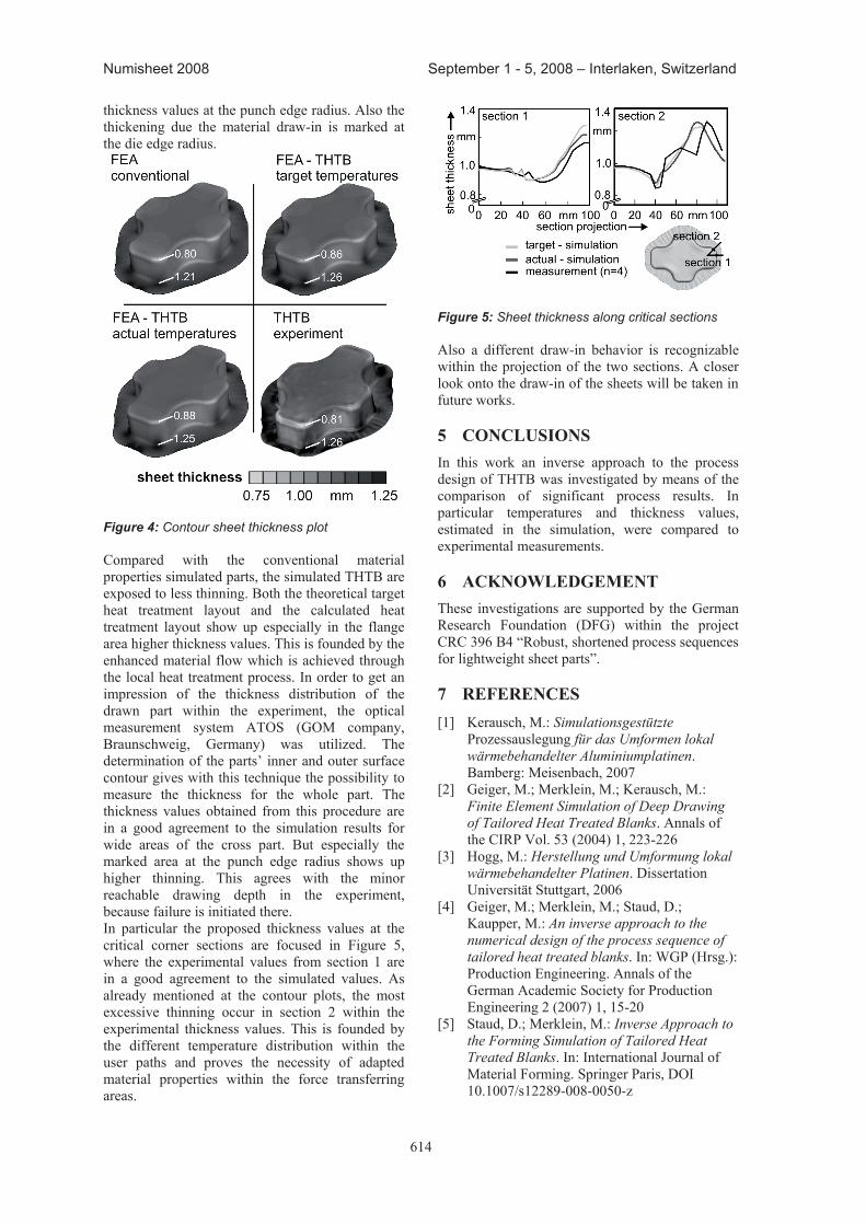
614


thickness values at the punch edge radius. Also the thickening due the material draw-in is marked at the die edge radius.

Figure 4: Contour sheet thickness plot Compared with the conventional material properties simulated parts, the simulated THTB are exposed to less thinning. Both the theoretical target heat treatment layout and the calculated heat treatment layout show up especially in the flange area higher thickness values. This is founded by the enhanced material flow which is achieved through the local heat treatment process. In order to get an impression of the thickness distribution of the drawn part within the experiment, the optical measurement system ATOS (GOM company, Braunschweig, Germany) was utilized. The determination of the parts’ inner and outer surface contour gives with this technique the possibility to measure the thickness for the whole part. The thickness values obtained from this procedure are in a good agreement to the simulation results for wide areas of the cross part. But especially the marked area at the punch edge radius shows up higher thinning. This agrees with the minor reachable drawing depth in the experiment, because failure is initiated there. In particular the proposed thickness values at the critical corner sections are focused in Figure 5, where the experimental values from section 1 are in a good agreement to the simulated values. As already mentioned at the contour plots, the most excessive thinning occur in section 2 within the experimental thickness values. This is founded by the different temperature distribution within the user paths and proves the necessity of adapted material properties within the force transferring areas.

Figure 5: Sheet thickness along critical sections Also a different draw-in behavior is recognizable within the projection of the two sections. A closer look onto the draw-in of the sheets will be taken in future works. 5 CONCLUSIONS In this work an inverse approach to the process design of THTB was investigated by means of the comparison of significant process results. In particular temperatures and thickness values, estimated in the simulation, were compared to experimental measurements. 6 ACKNOWLEDGEMENT These investigations are supported by the German Research Foundation (DFG) within the project CRC 396 B4 “Robust, shortened process sequences for lightweight sheet parts”. 7 REFERENCES [1] Kerausch, M.: Simulationsgestützte

Prozessauslegung für das Umformen lokal wärmebehandelter Aluminiumplatinen. Bamberg: Meisenbach, 2007

[2] Geiger, M.; Merklein, M.; Kerausch, M.: Finite Element Simulation of Deep Drawing of Tailored Heat Treated Blanks. Annals of the CIRP Vol. 53 (2004) 1, 223-226

[3] Hogg, M.: Herstellung und Umformung lokal wärmebehandelter Platinen. Dissertation Universität Stuttgart, 2006

[4] Geiger, M.; Merklein, M.; Staud, D.; Kaupper, M.: An inverse approach to the numerical design of the process sequence of tailored heat treated blanks. In: WGP (Hrsg.): Production Engineering. Annals of the German Academic Society for Production Engineering 2 (2007) 1, 15-20

[5] Staud, D.; Merklein, M.: Inverse Approach to the Forming Simulation of Tailored Heat Treated Blanks. In: International Journal of Material Forming. Springer Paris, DOI 10.1007/s12289-008-0050-z

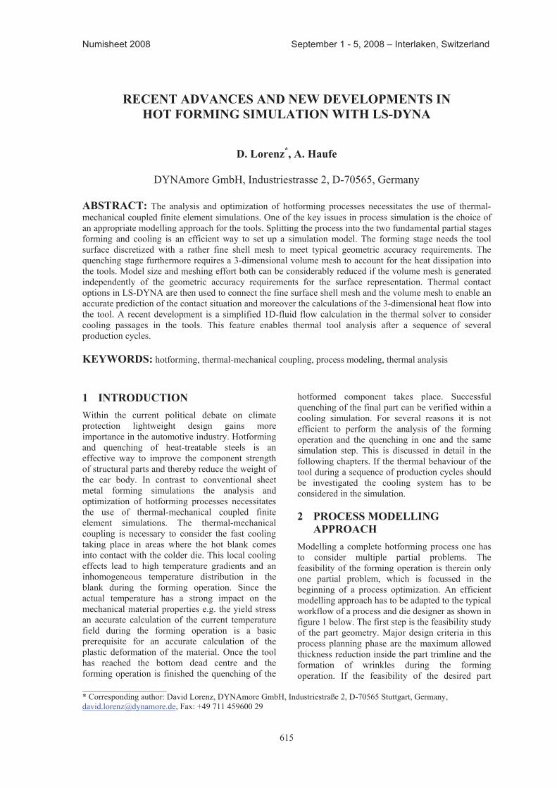
615


____________________* Corresponding author: David Lorenz, DYNAmore GmbH, Industriestraße 2, D-70565 Stuttgart, Germany, [email protected], Fax: +49 711 459600 29

reCeNt aDVaNCeS aND NeW DeVeLOpMeNtS IN hOt FOrMING SIMULatION WIth LS-DYNa

D. Lorenz*, a. haufe

DYNAmore GmbH, Industriestrasse 2, D-70565, Germany

aBStraCt: The analysis and optimization of hotforming processes necessitates the use of thermal-mechanical coupled finite element simulations. One of the key issues in process simulation is the choice of an appropriate modelling approach for the tools. Splitting the process into the two fundamental partial stages forming and cooling is an efficient way to set up a simulation model. The forming stage needs the tool surface discretized with a rather fine shell mesh to meet typical geometric accuracy requirements. The quenching stage furthermore requires a 3-dimensional volume mesh to account for the heat dissipation into the tools. Model size and meshing effort both can be considerably reduced if the volume mesh is generated independently of the geometric accuracy requirements for the surface representation. Thermal contact options in LS-DYNA are then used to connect the fine surface shell mesh and the volume mesh to enable an accurate prediction of the contact situation and moreover the calculations of the 3-dimensional heat flow into the tool. A recent development is a simplified 1D-fluid flow calculation in the thermal solver to consider cooling passages in the tools. This feature enables thermal tool analysis after a sequence of several production cycles.

KeYWOrDS: hotforming, thermal-mechanical coupling, process modeling, thermal analysis

1 INtrODUCtIONWithin the current political debate on climate protection lightweight design gains more importance in the automotive industry. Hotforming and quenching of heat-treatable steels is an effective way to improve the component strength of structural parts and thereby reduce the weight of the car body. In contrast to conventional sheet metal forming simulations the analysis and optimization of hotforming processes necessitates the use of thermal-mechanical coupled finite element simulations. The thermal-mechanical coupling is necessary to consider the fast cooling taking place in areas where the hot blank comes into contact with the colder die. This local cooling effects lead to high temperature gradients and an inhomogeneous temperature distribution in the blank during the forming operation. Since the actual temperature has a strong impact on the mechanical material properties e.g. the yield stress an accurate calculation of the current temperature field during the forming operation is a basic prerequisite for an accurate calculation of the plastic deformation of the material. Once the tool has reached the bottom dead centre and the forming operation is finished the quenching of the

hotformed component takes place. Successful quenching of the final part can be verified within a cooling simulation. For several reasons it is not efficient to perform the analysis of the forming operation and the quenching in one and the same simulation step. This is discussed in detail in the following chapters. If the thermal behaviour of the tool during a sequence of production cycles should be investigated the cooling system has to be considered in the simulation.

2 prOCeSS MODeLLING apprOaCh

Modelling a complete hotforming process one has to consider multiple partial problems. The feasibility of the forming operation is therein only one partial problem, which is focussed in the beginning of a process optimization. An efficient modelling approach has to be adapted to the typical workflow of a process and die designer as shown in figure 1 below. The first step is the feasibility study of the part geometry. Major design criteria in this process planning phase are the maximum allowed thickness reduction inside the part trimline and the formation of wrinkles during the forming operation. If the feasibility of the desired part

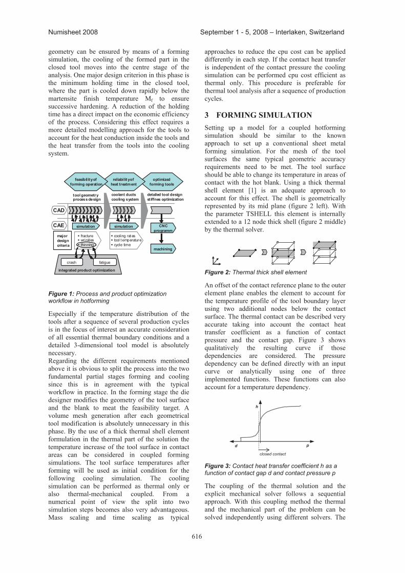
616


geometry can be ensured by means of a forming simulation, the cooling of the formed part in the closed tool moves into the centre stage of the analysis. One major design criterion in this phase is the minimum holding time in the closed tool, where the part is cooled down rapidly below the martensite finish temperature Mf to ensure successive hardening. A reduction of the holding time has a direct impact on the economic efficiency of the process. Considering this effect requires a more detailed modelling approach for the tools to account for the heat conduction inside the tools and the heat transfer from the tools into the cooling system.

optimizedforming tools

reliabilit yofheat treatment

simulation

tool geometryprocess design

simulation

fracturewrinklesthinning

cooling rat estool t emperaturecycle time

coolant ductscooling system

crash

CADCAD

CAECAE

majordesigncriteria

detailed tool designstiffnes optimization

feasibilityofforming operation

fatigue

integrated product optimization

CNCprogramm

machining

Figure 1: Process and product optimization workflow in hotforming

Especially if the temperature distribution of the tools after a sequence of several production cycles is in the focus of interest an accurate consideration of all essential thermal boundary conditions and a detailed 3-dimensional tool model is absolutely necessary. Regarding the different requirements mentioned above it is obvious to split the process into the two fundamental partial stages forming and cooling since this is in agreement with the typical workflow in practice. In the forming stage the die designer modifies the geometry of the tool surface and the blank to meat the feasibility target. A volume mesh generation after each geometrical tool modification is absolutely unnecessary in this phase. By the use of a thick thermal shell element formulation in the thermal part of the solution the temperature increase of the tool surface in contact areas can be considered in coupled forming simulations. The tool surface temperatures after forming will be used as initial condition for the following cooling simulation. The cooling simulation can be performed as thermal only or also thermal-mechanical coupled. From a numerical point of view the split into two simulation steps becomes also very advantageous. Mass scaling and time scaling as typical

approaches to reduce the cpu cost can be applied differently in each step. If the contact heat transfer is independent of the contact pressure the cooling simulation can be performed cpu cost efficient as thermal only. This procedure is preferable for thermal tool analysis after a sequence of production cycles.

3 FOrMING SIMULatION Setting up a model for a coupled hotforming simulation should be similar to the known approach to set up a conventional sheet metal forming simulation. For the mesh of the tool surfaces the same typical geometric accuracy requirements need to be met. The tool surface should be able to change its temperature in areas of contact with the hot blank. Using a thick thermal shell element [1] is an adequate approach to account for this effect. The shell is geometrically represented by its mid plane (figure 2 left). With the parameter TSHELL this element is internally extended to a 12 node thick shell (figure 2 middle) by the thermal solver.

Figure 2: Thermal thick shell element

An offset of the contact reference plane to the outer element plane enables the element to account for the temperature profile of the tool boundary layer using two additional nodes below the contact surface. The thermal contact can be described very accurate taking into account the contact heat transfer coefficient as a function of contact pressure and the contact gap. Figure 3 shows qualitatively the resulting curve if those dependencies are considered. The pressure dependency can be defined directly with an input curve or analytically using one of three implemented functions. These functions can also account for a temperature dependency.

pd

h

closed contact

Figure 3: Contact heat transfer coefficient h as a function of contact gap d and contact pressure p

The coupling of the thermal solution and the explicit mechanical solver follows a sequential approach. With this coupling method the thermal and the mechanical part of the problem can be solved independently using different solvers. The

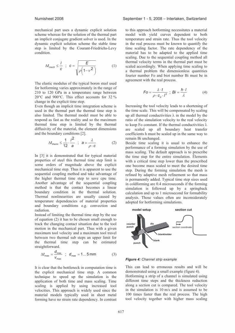
617


mechanical part uses a dynamic explicit solution scheme whereas for the solution of the thermal part an implicit conjugate gradient solver is used. In the dynamic explicit solution scheme the stable time step is limited by the Courant-Friedrichs-Levy condition.

21; Ec

cltmech (1)

The elastic modulus of the typical boron steel used for hotforming varies approximately in the range of 210 to 120 GPa in a temperature range between 20°C and 900°C. This effect accounts for 32 % change in the explicit time step. Even though an implicit time integration scheme is used in the thermal part the thermal time step is also limited. The thermal model must be able to respond as fast as the reality and so the maximum thermal time step is limited by the thermal diffusivity of the material, the element dimensions and the boundary conditions [2].

ca

alttherm ;2

121 (2)

In [3] it is demonstrated that for typical material properties of steel this thermal time step limit is some orders of magnitude above the explicit mechanical time step. Thus it is apparent to use the sequential coupling method and take advantage of the higher thermal time step to save cpu time. Another advantage of the sequential coupling method is that the contact becomes a linear boundary condition in the thermal solution. Thermal nonlinearities are usually caused by temperature dependencies of material properties and boundary conditions e.g. convection and radiation. Instead of limiting the thermal time step by the use of equation (2) it has to be chosen small enough to track the changing contact situation due to the tool motion in the mechanical part. Thus with a given maximum tool velocity and a maximum tool travel between two thermal sub steps an upper limit for the thermal time step can be estimated straightforward.

mm5...1; maxmax

maxmax d

vdt (3)

It is clear that the bottleneck in computation time is the explicit mechanical time step. A common technique to speed up the simulation is the application of both time and mass scaling. Time scaling is applied by using increased tool velocities. This approach is widely used since the material models typically used in sheet metal forming have no strain rate dependency. In contrast

to this approach hotforming necessitates a material model with yield curves dependent to both temperature and strain rate. Thus the tool velocity in the real process must be known to quantify the time scaling factor. The rate dependency of the material has to be adapted to the applied time scaling. Due to the sequential coupling method all thermal velocity terms in the thermal part must be scaled accordingly. When applying time scaling to a thermal problem the dimensionless quantities fourier number Fo and biot number Bi must be in agreement with the real process.

lhBilc

tFop

;2 (4)

Increasing the tool velocity leads to a shortening of the time scale. This will be compensated by scaling up all thermal conductivities in the model by the ratio of the simulation velocity to the real velocity to keep Fo constant. If the thermal conductivities are scaled up all boundary heat transfer coefficients h must be scaled up in the same way to remain Bi unchanged. Beside time scaling it is usual to enhance the performance of a forming simulation by the use of mass scaling. The default approach is to prescribe the time step for the entire simulation. Êlements with a critical time step lower than the prescribed one become mass scaled to meet the desired time step. During the forming simulation the mesh is refined by adaptive mesh refinement so that mass is permanently added. Typical time step sizes used in coldforming are 0.4 microseconds if the forming simulation is followed up by a springback calculation and up to 1 microsecond for formability analysis. Those values often are inconsiderately adopted for hotforming simulations.

section cut

section coordinatediecounter

punch

punch

blankholder

blank

model setup

Figure 4: Channel strip example

This can lead to erroneous results and will be demonstrated using a small example (figure 4). Hotforming a strip of a channel is simulated using different time steps and the thickness reduction along a section cut is compared. The tool velocity in the simulation is 10 m/s and is assumed to be 100 times faster than the real process. The high tool velocity together with higher mass scaling

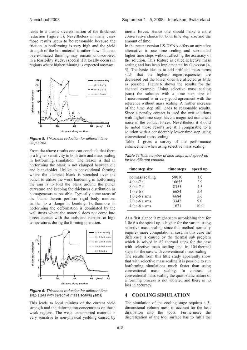
618


leads to a drastic overestimation of the thickness reduction (figure 5). Nevertheless in many cases those results seem to be reasonable because the friction in hotforming is very high and the yield strength of the hot material is rather slow. Thus an overestimated thinning may remain undiscovered in a feasibility study, especial if it locally occurs in regions where higher thinning is expected anyway.

20

15

10

5

00 20 40 60 80

20

15

10

5

00 20 40 60 80

distance along section

thic

knes

s re

duct

ion

[%]

[mm]

no mass scalingno mass scaling

dt = 4.0 e-7 s

dt = 8.0 e-7 s

dt = 1.0 e-6 s

Figure 5: Thickness reduction for different time step sizes

From the above results one can conclude that there is a higher sensitivity to both time and mass scaling in hotforming simulation. The reason is that in hotforming the blank is not clamped between die and blankholder. Unlike in conventional forming where the clamped blank is stretched over the punch to utilize the work hardening in hotforming the aim is to fold the blank around the punch curvature and keeping the thickness distribution as homogeneous as possible. Typically some areas of the blank therein perform rigid body motions similar to a flange in bending. Furthermore in hotforming the deformation is dominated by the wall areas where the material does not come into direct contact with the tools and remains at high temperatures during the forming operation.

4

3

2

1

00 20 40 60 80

distance along section

thic

knes

s re

duct

ion

[%]

[mm]

5no mass scaling

dt = 1.0 e-6 s sms

dt = 2.0 e-6 s sms

dt = 4.0 e-6 s sms

dt = 4.0 e-7 s

Figure 6: Thickness reduction for different time step sizes with selective mass scaling (sms)

This leads to local minima of the current yield strength and the deformation concentrates on those weak regions. The weak unsupported material is very sensitive to non-physical yielding caused by

inertia forces. Hence one should make a more conservative choice for both time step size and the amount of time. In the recent version LS-DYNA offers an attractive alternative to use time scaling and substantial higher time steps without affecting the accuracy of the solution. This feature is called selective mass scaling and has been implemented by Olovsson [4, 5]. The basic idea is to add artificial mass terms such that the highest eigenfrequencies are decreased but the lower ones are affected as little as possible. Figure 6 shows the results for the channel example. Using selective mass scaling (sms) the solution with a time step size of 1 microsecond is in very good agreement with the reference without mass scaling. A further increase of the time step still leads to reasonable results. Since a penalty contact is used the two solutions with higher time steps have a magnified numerical noise in the contact forces. Nevertheless it should be noted those results are still comparable to a solution with a considerably lower time step using conventional mass scaling Table 1 gives a survey of the performance enhancement when using selective mass scaling.

Table 1: Total number of time steps and speed-up for the different variants

time step size time steps speed up

no mass scaling 58010 1.0 4.0 e-7 s 16655 2.9 8.0 e-7 s 8355 4.5 1.0 e-6 s 6684 5.4 1.0 e-6 s sms 6684 5.6 2.0 e-6 s sms 3342 9.0 4.0 e-6 s sms 1671 10.9

At a first glance it might seem astonishing that for 1.0e-6 s the speed-up is higher for the variant using selective mass scaling since this method normally requires more computational cost. In this case the difference is caused by the thermal sub problem which is solved in 82 thermal steps for the case with selective mass scaling and in 104 thermal steps for the case with conventional mass scaling. The results from this little study apparently show that with selective mass scaling it is possible to run hotforming simulations much faster than using conventional mass scaling. In contrast to conventional mass scaling the quasi-static nature of a forming process is not violated and there is no loss in accuracy.

4 COOLING SIMULatION The simulation of the cooling stage requires a 3-dimensional volume mesh to account for the heat dissipation into the tools. Furthermore the discretization of the tool surface has to fulfil the

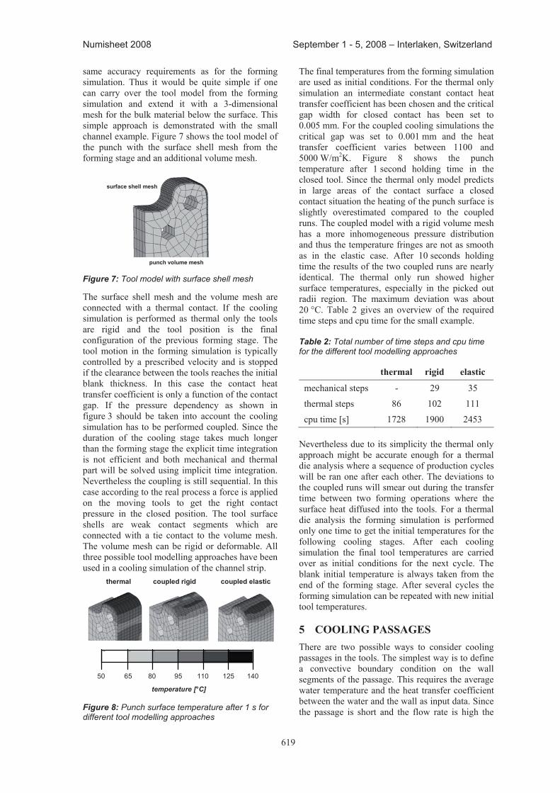
619


same accuracy requirements as for the forming simulation. Thus it would be quite simple if one can carry over the tool model from the forming simulation and extend it with a 3-dimensional mesh for the bulk material below the surface. This simple approach is demonstrated with the small channel example. Figure 7 shows the tool model of the punch with the surface shell mesh from the forming stage and an additional volume mesh.

surface shell mesh

punch volume mesh

Figure 7: Tool model with surface shell mesh

The surface shell mesh and the volume mesh are connected with a thermal contact. If the cooling simulation is performed as thermal only the tools are rigid and the tool position is the final configuration of the previous forming stage. The tool motion in the forming simulation is typically controlled by a prescribed velocity and is stopped if the clearance between the tools reaches the initial blank thickness. In this case the contact heat transfer coefficient is only a function of the contact gap. If the pressure dependency as shown in figure 3 should be taken into account the cooling simulation has to be performed coupled. Since the duration of the cooling stage takes much longer than the forming stage the explicit time integration is not efficient and both mechanical and thermal part will be solved using implicit time integration. Nevertheless the coupling is still sequential. In this case according to the real process a force is applied on the moving tools to get the right contact pressure in the closed position. The tool surface shells are weak contact segments which are connected with a tie contact to the volume mesh. The volume mesh can be rigid or deformable. All three possible tool modelling approaches have been used in a cooling simulation of the channel strip.

50 65 80 95 110 125 140

temperature [°C]

thermal coupled rigid coupled elastic

Figure 8: Punch surface temperature after 1 s for different tool modelling approaches

The final temperatures from the forming simulation are used as initial conditions. For the thermal only simulation an intermediate constant contact heat transfer coefficient has been chosen and the critical gap width for closed contact has been set to 0.005 mm. For the coupled cooling simulations the critical gap was set to 0.001 mm and the heat transfer coefficient varies between 1100 and 5000 W/m2K. Figure 8 shows the punch temperature after 1 second holding time in the closed tool. Since the thermal only model predicts in large areas of the contact surface a closed contact situation the heating of the punch surface is slightly overestimated compared to the coupled runs. The coupled model with a rigid volume mesh has a more inhomogeneous pressure distribution and thus the temperature fringes are not as smooth as in the elastic case. After 10 seconds holding time the results of the two coupled runs are nearly identical. The thermal only run showed higher surface temperatures, especially in the picked out radii region. The maximum deviation was about 20 °C. Table 2 gives an overview of the required time steps and cpu time for the small example.

Table 2: Total number of time steps and cpu time for the different tool modelling approaches

thermal rigid elastic

mechanical steps - 29 35

thermal steps 86 102 111

cpu time [s] 1728 1900 2453

Nevertheless due to its simplicity the thermal only approach might be accurate enough for a thermal die analysis where a sequence of production cycles will be ran one after each other. The deviations to the coupled runs will smear out during the transfer time between two forming operations where the surface heat diffused into the tools. For a thermal die analysis the forming simulation is performed only one time to get the initial temperatures for the following cooling stages. After each cooling simulation the final tool temperatures are carried over as initial conditions for the next cycle. The blank initial temperature is always taken from the end of the forming stage. After several cycles the forming simulation can be repeated with new initial tool temperatures.

5 COOLING paSSaGeS There are two possible ways to consider cooling passages in the tools. The simplest way is to define a convective boundary condition on the wall segments of the passage. This requires the average water temperature and the heat transfer coefficient between the water and the wall as input data. Since the passage is short and the flow rate is high the

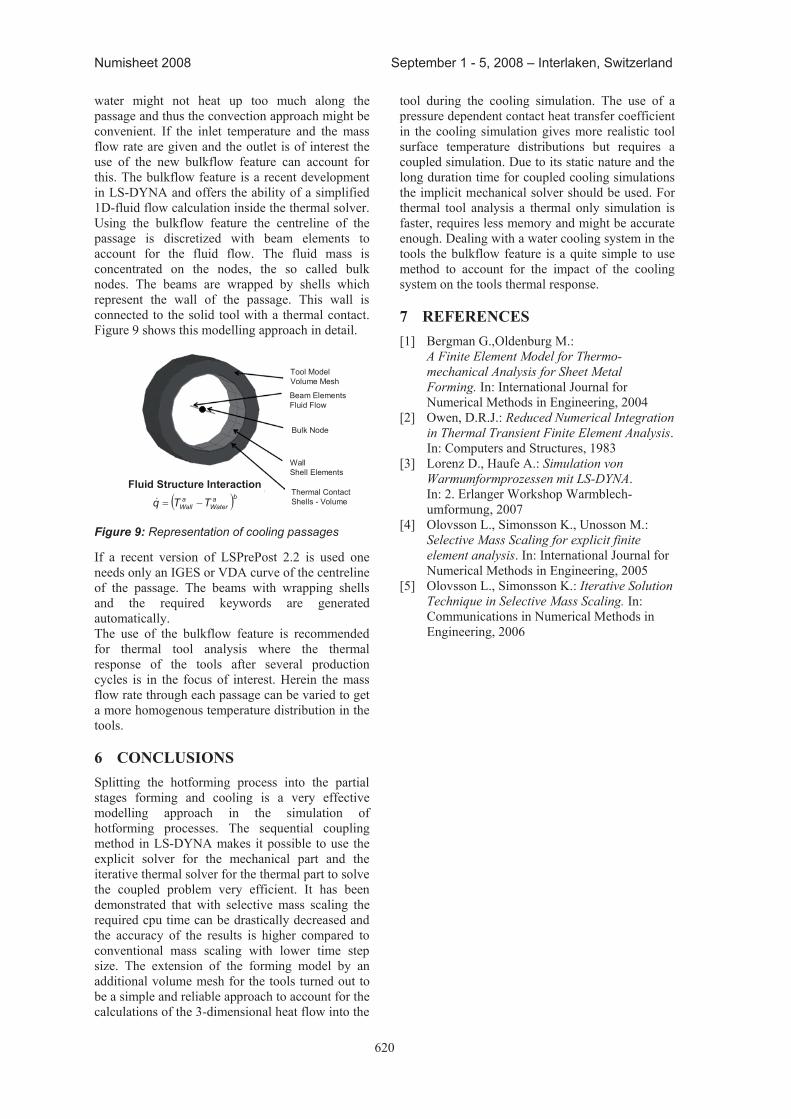
620


water might not heat up too much along the passage and thus the convection approach might be convenient. If the inlet temperature and the mass flow rate are given and the outlet is of interest the use of the new bulkflow feature can account for this. The bulkflow feature is a recent development in LS-DYNA and offers the ability of a simplified 1D-fluid flow calculation inside the thermal solver. Using the bulkflow feature the centreline of the passage is discretized with beam elements to account for the fluid flow. The fluid mass is concentrated on the nodes, the so called bulk nodes. The beams are wrapped by shells which represent the wall of the passage. This wall is connected to the solid tool with a thermal contact. Figure 9 shows this modelling approach in detail.

Tool ModelVolume Mesh

Beam ElementsFluid Flow

Bulk Node

WallShell Elements

Thermal ContactShells - Volume

baWater

aWall TTq

Fluid Structure Interaction

Figure 9: Representation of cooling passages

If a recent version of LSPrePost 2.2 is used one needs only an IGES or VDA curve of the centreline of the passage. The beams with wrapping shells and the required keywords are generated automatically. The use of the bulkflow feature is recommended for thermal tool analysis where the thermal response of the tools after several production cycles is in the focus of interest. Herein the mass flow rate through each passage can be varied to get a more homogenous temperature distribution in the tools.

6 CONCLUSIONS Splitting the hotforming process into the partial stages forming and cooling is a very effective modelling approach in the simulation of hotforming processes. The sequential coupling method in LS-DYNA makes it possible to use the explicit solver for the mechanical part and the iterative thermal solver for the thermal part to solve the coupled problem very efficient. It has been demonstrated that with selective mass scaling the required cpu time can be drastically decreased and the accuracy of the results is higher compared to conventional mass scaling with lower time step size. The extension of the forming model by an additional volume mesh for the tools turned out to be a simple and reliable approach to account for the calculations of the 3-dimensional heat flow into the

tool during the cooling simulation. The use of a pressure dependent contact heat transfer coefficient in the cooling simulation gives more realistic tool surface temperature distributions but requires a coupled simulation. Due to its static nature and the long duration time for coupled cooling simulations the implicit mechanical solver should be used. For thermal tool analysis a thermal only simulation is faster, requires less memory and might be accurate enough. Dealing with a water cooling system in the tools the bulkflow feature is a quite simple to use method to account for the impact of the cooling system on the tools thermal response.

7 reFereNCeS [1] Bergman G.,Oldenburg M.:

A Finite Element Model for Thermo-mechanical Analysis for Sheet Metal Forming. In: International Journal for Numerical Methods in Engineering, 2004

[2] Owen, D.R.J.: Reduced Numerical Integration in Thermal Transient Finite Element Analysis.In: Computers and Structures, 1983

[3] Lorenz D., Haufe A.: Simulation von Warmumformprozessen mit LS-DYNA.

In: 2. Erlanger Workshop Warmblech-umformung, 2007

[4] Olovsson L., Simonsson K., Unosson M.: Selective Mass Scaling for explicit finite element analysis. In: International Journal for Numerical Methods in Engineering, 2005

[5] Olovsson L., Simonsson K.: Iterative Solution Technique in Selective Mass Scaling. In: Communications in Numerical Methods in Engineering, 2006

621


____________________ * Corresponding author: Institute Tools & Forming, Graz University of Technology, Inffeldgasse 11/1, 8010 Graz, mail: [email protected]

aLterNatIVe apprOaCheS FOr the SIMULatION OF the

hOt FOrMING prOCeSS

Kolleck, r., Löscher, h., Veit, r., Weiß, W.*

Graz University of Technology, Institute Tools & Forming aBStraCt: As a rising number of components is being produced via a hot forming process, there is an increasing interest in a complete virtual representation of the process. In the following paper the possibilities for the remodelling of the hot forming process are examined. The most important parameters and their consideration in commercial FE tools are presented and discussed. The currently available simulations tools come with significant simplications of physical processes and particularly in terms of thermo-mechanical coupling. An alternative approach is found in the CFD simulation. This paper describes an approach for the design of press hardening tools based on a coupled CFD and forming simulation. The forming simulation allows a prediction of part failures during production and the optimal tool topology can be attained. By the consideration of thermodynamic and fluid mechanical principles in the CFD simulation the performance of the cooling system can be optimized, considering the planned technology for the production of the tool. The coupling of both simulation systems offers the possibility to consider all relevant boundary conditions and also the interactions between them. Consequently, a more precise prediction of the press hardening process and forming outcome, and an optimum tool design is possible.

KeYWOrDS: Hot forming, Thermo-mechanical coupling, CFD 1 INtrODUCtIONShorter and shorter development times and the demand for an optimized press hardening process requires the use of virtual development tools. The increased use of hot forming components makes further development of new or already existing simulation tools inevitable. The purpose of these tools is a better forecast of the feasibility of a part and the performance of the ‘heat exchanger’ press hardening tool. This presupposes the virtual representation of the complete process. Therefore, the design of cooled forming tools confronts the engineer with new challenges. If the required cooling capacity is not reached, cycle times increase and consequently component costs increase. Besides shorter cooling times, a uniform temperature distribution must be ensured, i.e., ‘hot spots’ on the tools and the component must be avoided. This requires an optimal lay-out of the cooling channel geometry. It turns out that the CFD simulation offers a comprehensive possibility to design an optimal heat exchanger layout. 2 State OF the art In comparison with cold forming the physical system of hot forming is considerably more complex [1]. For the analysis of the hot forming

process the examination of all relevant parameters that describe the press hardening process, is necessary. Commercial FEM software packages for the evaluation of the feasibility of component geometries confine themselves to a simplified representation of the press hardening process. An important precondition for the evaluation of the feasibility of a press hardened component is the consideration of strain dependent yield stress curves with dependence on the sheet temperature and different materials [2]. Furthermore, critical to a part feasibility study is the start temperature of the martensitic phase transformation [3]. The temperature must not fall below 400°C [11] during the forming process due to low deformability of the martensitic phase. As parameters like the thermal conductivity k and the specific heat capacity cp tend to be strongly temperature dependent, an exact representation of the temperature profile is useful, and in fact, necessary. In the commercially available simulation programs, the tool temperatures are often not calculated but provided by the user [4]. This leads to a strong simplification of the physical process. Equation (1), a heat transfer equation in 3D, assumes temperature independent material parameters as a simplification.

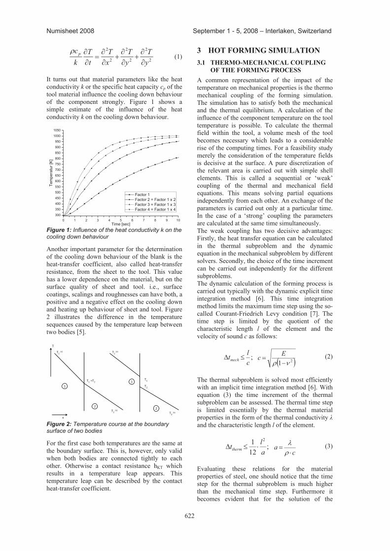
622


2

2

2

2

2

2

yT

yT

xT

tT

kcp (1)

It turns out that material parameters like the heat conductivity k or the specific heat capacity cp of the tool material influence the cooling down behaviour of the component strongly. Figure 1 shows a simple estimate of the influence of the heat conductivity k on the cooling down behaviour.

0 1 2 3 4 5 6 7 8 9 10300

350

400

450

500

550

600

650

700

750

800

850

900

950

1000

1050

Tem

pera

tur [

K]

Time [sec]

Factor 1 Factor 2 = Factor 1 x 2 Factor 3 = Factor 1 x 3 Factor 4 = Factor 1 x 4

Figure 1: Influence of the heat conductivity k on the cooling down behaviour

Another important parameter for the determination of the cooling down behaviour of the blank is the heat-transfer coefficient, also called heat-transfer resistance, from the sheet to the tool. This value has a lower dependence on the material, but on the surface quality of sheet and tool. i.e., surface coatings, scalings and roughnesses can have both, a positive and a negative effect on the cooling down and heating up behaviour of sheet and tool. Figure 2 illustrates the difference in the temperature sequences caused by the temperature leap between two bodies [5].

1

2

T1 (x)

T1 =T2

T2 (x)

x

T

1

T1 (x)

T1

T2

2T2 (x)

Figure 2: Temperature course at the boundary surface of two bodies

For the first case both temperatures are the same at the boundary surface. This is, however, only valid when both bodies are connected tightly to each other. Otherwise a contact resistance hKT which results in a temperature leap appears. This temperature leap can be described by the contact heat-transfer coefficient.

3 hOt FOrMING SIMULatION 3.1 therMO-MeChaNICaL COUpLING

OF the FOrMING prOCeSS A common representation of the impact of the temperature on mechanical properties is the thermo mechanical coupling of the forming simulation. The simulation has to satisfy both the mechanical and the thermal equilibrium. A calculation of the influence of the component temperature on the tool temperature is possible. To calculate the thermal field within the tool, a volume mesh of the tool becomes necessary which leads to a considerable rise of the computing times. For a feasibility study merely the consideration of the temperature fields is decisive at the surface. A pure discretization of the relevant area is carried out with simple shell elements. This is called a sequential or ‘weak’ coupling of the thermal and mechanical field equations. This means solving partial equations independently from each other. An exchange of the parameters is carried out only at a particular time. In the case of a ‘strong’ coupling the parameters are calculated at the same time simultaneously. The weak coupling has two decisive advantages: Firstly, the heat transfer equation can be calculated in the thermal subproblem and the dynamic equation in the mechanical subproblem by different solvers. Secondly, the choice of the time increment can be carried out independently for the different subproblems. The dynamic calculation of the forming process is carried out typically with the dynamic explicit time integration method [6]. This time integration method limits the maximum time step using the so-called Courant-Friedrich Levy condition [7]. The time step is limited by the quotient of the characteristic length l of the element and the velocity of sound c as follows:

;cltmech

21Ec (2)

The thermal subproblem is solved most efficiently with an implicit time integration method [6]. With equation (3) the time increment of the thermal subproblem can be assessed. The thermal time step is limited essentially by the thermal material properties in the form of the thermal conductivity and the characteristic length l of the element.

;121 2

alttherm

ca (3)

Evaluating these relations for the material properties of steel, one should notice that the time step for the thermal subproblem is much higher than the mechanical time step. Furthermore it becomes evident that for the solution of the

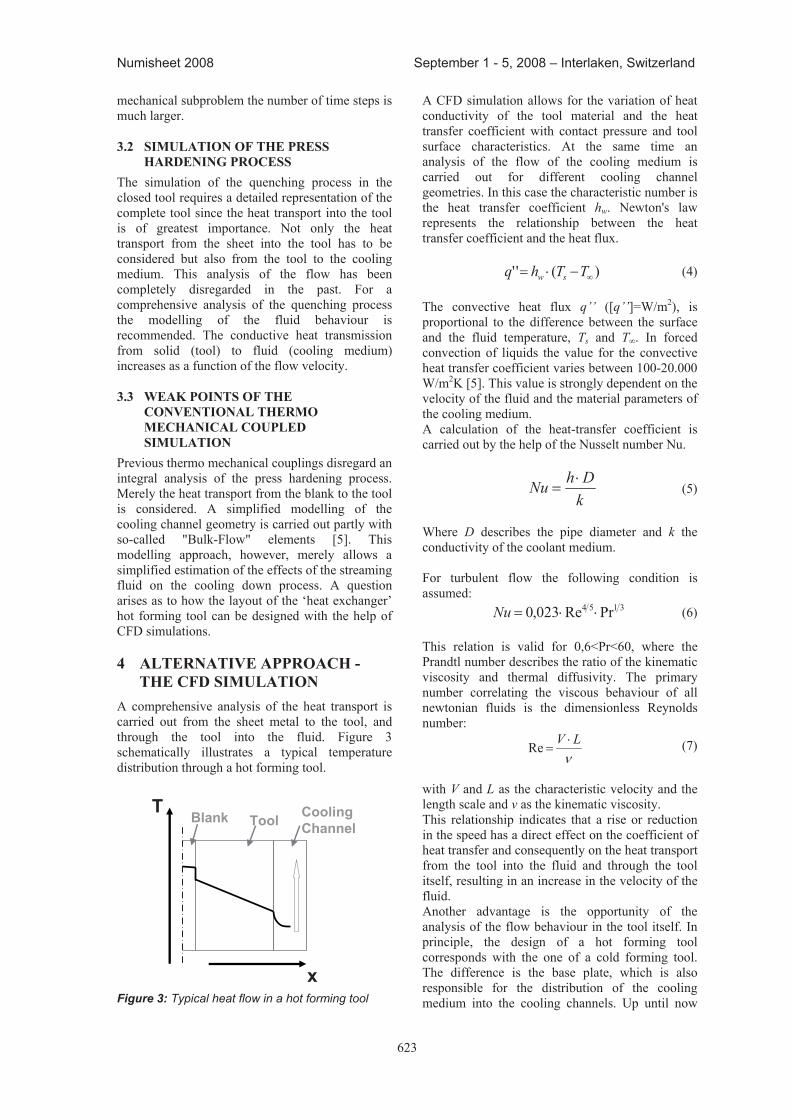
623


mechanical subproblem the number of time steps is much larger. 3.2 SIMULatION OF the preSS

harDeNING prOCeSS The simulation of the quenching process in the closed tool requires a detailed representation of the complete tool since the heat transport into the tool is of greatest importance. Not only the heat transport from the sheet into the tool has to be considered but also from the tool to the cooling medium. This analysis of the flow has been completely disregarded in the past. For a comprehensive analysis of the quenching process the modelling of the fluid behaviour is recommended. The conductive heat transmission from solid (tool) to fluid (cooling medium) increases as a function of the flow velocity. 3.3 WeaK pOINtS OF the

CONVeNtIONaL therMO MeChaNICaL COUpLeD SIMULatION

Previous thermo mechanical couplings disregard an integral analysis of the press hardening process. Merely the heat transport from the blank to the tool is considered. A simplified modelling of the cooling channel geometry is carried out partly with so-called "Bulk-Flow" elements [5]. This modelling approach, however, merely allows a simplified estimation of the effects of the streaming fluid on the cooling down process. A question arises as to how the layout of the ‘heat exchanger’ hot forming tool can be designed with the help of CFD simulations. 4 aLterNatIVe apprOaCh -

the CFD SIMULatION A comprehensive analysis of the heat transport is carried out from the sheet metal to the tool, and through the tool into the fluid. Figure 3 schematically illustrates a typical temperature distribution through a hot forming tool.

Blank Tool CoolingChannel

x

T

Figure 3: Typical heat flow in a hot forming tool

A CFD simulation allows for the variation of heat conductivity of the tool material and the heat transfer coefficient with contact pressure and tool surface characteristics. At the same time an analysis of the flow of the cooling medium is carried out for different cooling channel geometries. In this case the characteristic number is the heat transfer coefficient hw. Newton's law represents the relationship between the heat transfer coefficient and the heat flux.

)('' TThq sw (4) The convective heat flux q’’ ([q’’]=W/m2), is proportional to the difference between the surface and the fluid temperature, Ts and T∞. In forced convection of liquids the value for the convective heat transfer coefficient varies between 100-20.000 W/m2K [5]. This value is strongly dependent on the velocity of the fluid and the material parameters of the cooling medium. A calculation of the heat-transfer coefficient is carried out by the help of the Nusselt number Nu.

kDhNu (5)

Where D describes the pipe diameter and k the conductivity of the coolant medium. For turbulent flow the following condition is assumed:

3154 PrRe023,0Nu (6) This relation is valid for 0,6<Pr<60, where the Prandtl number describes the ratio of the kinematic viscosity and thermal diffusivity. The primary number correlating the viscous behaviour of all newtonian fluids is the dimensionless Reynolds number:

LVRe (7)

with V and L as the characteristic velocity and the length scale and as the kinematic viscosity. This relationship indicates that a rise or reduction in the speed has a direct effect on the coefficient of heat transfer and consequently on the heat transport from the tool into the fluid and through the tool itself, resulting in an increase in the velocity of the fluid. Another advantage is the opportunity of the analysis of the flow behaviour in the tool itself. In principle, the design of a hot forming tool corresponds with the one of a cold forming tool. The difference is the base plate, which is also responsible for the distribution of the cooling medium into the cooling channels. Up until now

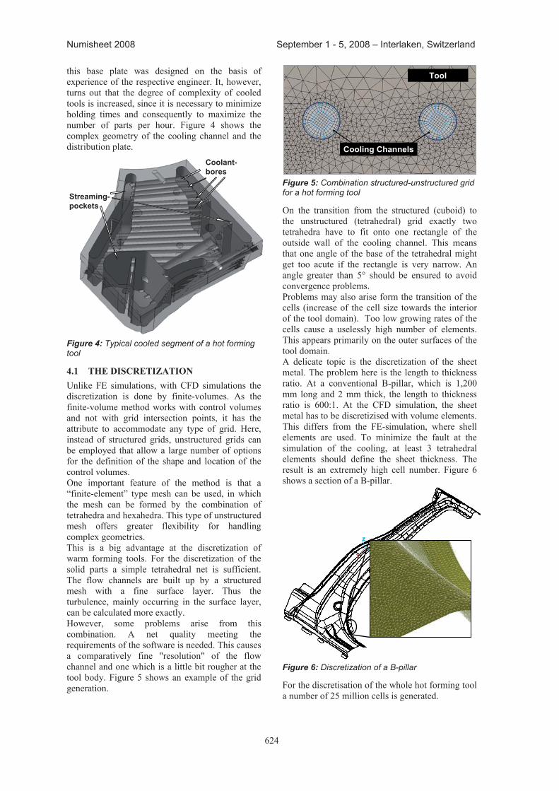
624


this base plate was designed on the basis of experience of the respective engineer. It, however, turns out that the degree of complexity of cooled tools is increased, since it is necessary to minimize holding times and consequently to maximize the number of parts per hour. Figure 4 shows the complex geometry of the cooling channel and the distribution plate.

Streaming-pockets

Coolant-bores

Figure 4: Typical cooled segment of a hot forming tool

4.1 the DISCretIZatION Unlike FE simulations, with CFD simulations the discretization is done by finite-volumes. As the finite-volume method works with control volumes and not with grid intersection points, it has the attribute to accommodate any type of grid. Here, instead of structured grids, unstructured grids can be employed that allow a large number of options for the definition of the shape and location of the control volumes. One important feature of the method is that a “finite-element” type mesh can be used, in which the mesh can be formed by the combination of tetrahedra and hexahedra. This type of unstructured mesh offers greater flexibility for handling complex geometries. This is a big advantage at the discretization of warm forming tools. For the discretization of the solid parts a simple tetrahedral net is sufficient. The flow channels are built up by a structured mesh with a fine surface layer. Thus the turbulence, mainly occurring in the surface layer, can be calculated more exactly. However, some problems arise from this combination. A net quality meeting the requirements of the software is needed. This causes a comparatively fine "resolution" of the flow channel and one which is a little bit rougher at the tool body. Figure 5 shows an example of the grid generation.

Cooling Channels

Tool

Figure 5: Combination structured-unstructured grid for a hot forming tool

On the transition from the structured (cuboid) to the unstructured (tetrahedral) grid exactly two tetrahedra have to fit onto one rectangle of the outside wall of the cooling channel. This means that one angle of the base of the tetrahedral might get too acute if the rectangle is very narrow. An angle greater than 5° should be ensured to avoid convergence problems. Problems may also arise form the transition of the cells (increase of the cell size towards the interior of the tool domain). Too low growing rates of the cells cause a uselessly high number of elements. This appears primarily on the outer surfaces of the tool domain. A delicate topic is the discretization of the sheet metal. The problem here is the length to thickness ratio. At a conventional B-pillar, which is 1,200 mm long and 2 mm thick, the length to thickness ratio is 600:1. At the CFD simulation, the sheet metal has to be discretizised with volume elements. This differs from the FE-simulation, where shell elements are used. To minimize the fault at the simulation of the cooling, at least 3 tetrahedral elements should define the sheet thickness. The result is an extremely high cell number. Figure 6 shows a section of a B-pillar.

Figure 6: Discretization of a B-pillar

For the discretisation of the whole hot forming tool a number of 25 million cells is generated.

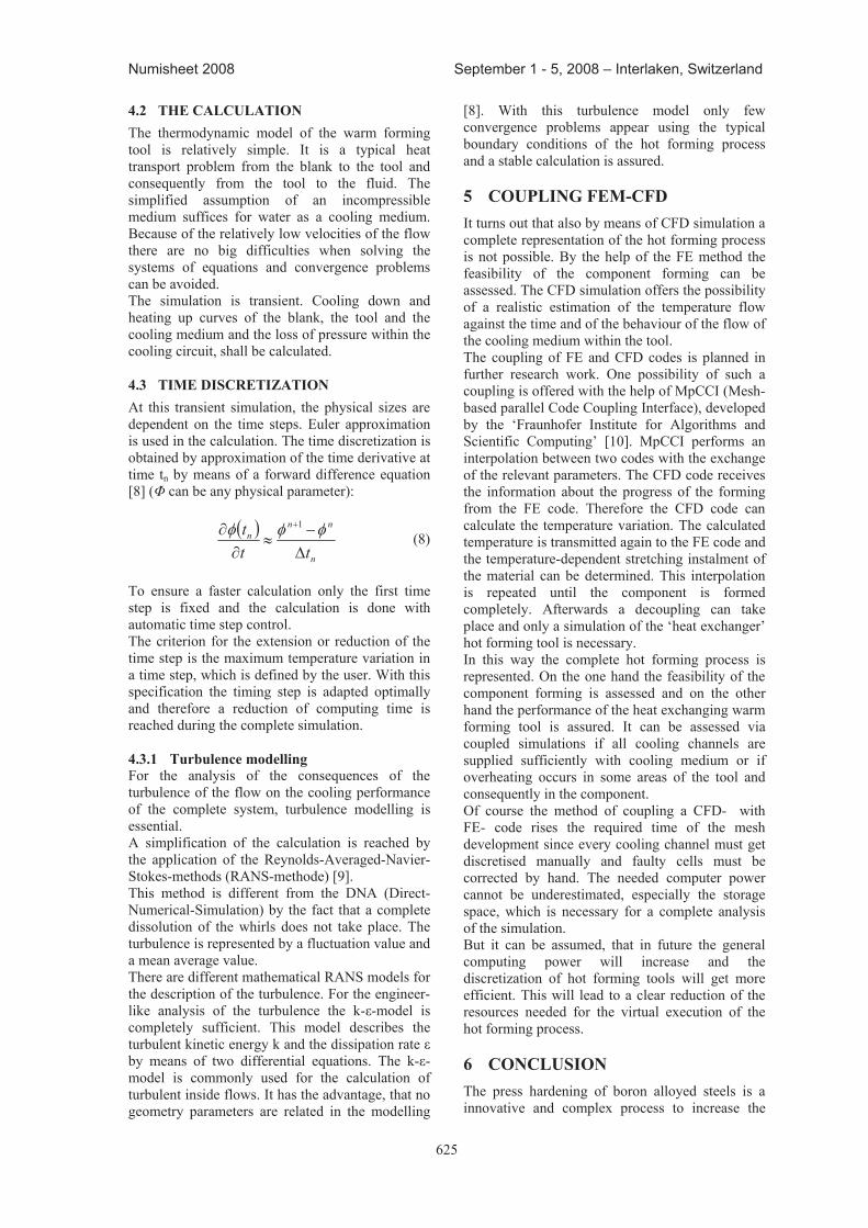
625


4.2 the CaLCULatION The thermodynamic model of the warm forming tool is relatively simple. It is a typical heat transport problem from the blank to the tool and consequently from the tool to the fluid. The simplified assumption of an incompressible medium suffices for water as a cooling medium. Because of the relatively low velocities of the flow there are no big difficulties when solving the systems of equations and convergence problems can be avoided. The simulation is transient. Cooling down and heating up curves of the blank, the tool and the cooling medium and the loss of pressure within the cooling circuit, shall be calculated. 4.3 tIMe DISCretIZatION At this transient simulation, the physical sizes are dependent on the time steps. Euler approximation is used in the calculation. The time discretization is obtained by approximation of the time derivative at time tn by means of a forward difference equation [8] ( can be any physical parameter):

n

nnn

ttt 1

(8)

To ensure a faster calculation only the first time step is fixed and the calculation is done with automatic time step control. The criterion for the extension or reduction of the time step is the maximum temperature variation in a time step, which is defined by the user. With this specification the timing step is adapted optimally and therefore a reduction of computing time is reached during the complete simulation. 4.3.1 turbulence modelling For the analysis of the consequences of the turbulence of the flow on the cooling performance of the complete system, turbulence modelling is essential. A simplification of the calculation is reached by the application of the Reynolds-Averaged-Navier-Stokes-methods (RANS-methode) [9]. This method is different from the DNA (Direct-Numerical-Simulation) by the fact that a complete dissolution of the whirls does not take place. The turbulence is represented by a fluctuation value and a mean average value. There are different mathematical RANS models for the description of the turbulence. For the engineer-like analysis of the turbulence the k-ε-model is completely sufficient. This model describes the turbulent kinetic energy k and the dissipation rate ε by means of two differential equations. The k-ε-model is commonly used for the calculation of turbulent inside flows. It has the advantage, that no geometry parameters are related in the modelling

[8]. With this turbulence model only few convergence problems appear using the typical boundary conditions of the hot forming process and a stable calculation is assured. 5 COUpLING FeM-CFD It turns out that also by means of CFD simulation a complete representation of the hot forming process is not possible. By the help of the FE method the feasibility of the component forming can be assessed. The CFD simulation offers the possibility of a realistic estimation of the temperature flow against the time and of the behaviour of the flow of the cooling medium within the tool. The coupling of FE and CFD codes is planned in further research work. One possibility of such a coupling is offered with the help of MpCCI (Mesh-based parallel Code Coupling Interface), developed by the ‘Fraunhofer Institute for Algorithms and Scientific Computing’ [10]. MpCCI performs an interpolation between two codes with the exchange of the relevant parameters. The CFD code receives the information about the progress of the forming from the FE code. Therefore the CFD code can calculate the temperature variation. The calculated temperature is transmitted again to the FE code and the temperature-dependent stretching instalment of the material can be determined. This interpolation is repeated until the component is formed completely. Afterwards a decoupling can take place and only a simulation of the ‘heat exchanger’ hot forming tool is necessary. In this way the complete hot forming process is represented. On the one hand the feasibility of the component forming is assessed and on the other hand the performance of the heat exchanging warm forming tool is assured. It can be assessed via coupled simulations if all cooling channels are supplied sufficiently with cooling medium or if overheating occurs in some areas of the tool and consequently in the component. Of course the method of coupling a CFD- with FE- code rises the required time of the mesh development since every cooling channel must get discretised manually and faulty cells must be corrected by hand. The needed computer power cannot be underestimated, especially the storage space, which is necessary for a complete analysis of the simulation. But it can be assumed, that in future the general computing power will increase and the discretization of hot forming tools will get more efficient. This will lead to a clear reduction of the resources needed for the virtual execution of the hot forming process. 6 CONCLUSION The press hardening of boron alloyed steels is a innovative and complex process to increase the

626


strength of critical body parts. It is reached through a structural transformation from austenite into martensite. The complete simulation of the hot forming process is a very complex topic with parameters influencing each other. Among others the heat transfer coefficient from the blank to the tool and the temperature-dependent stretching instalment have to be taken into account. Meanwhile, these parameters can at least be represented in simplified terms in the virtual modelling of the hot forming process. Thermo-mechanical coupling only gives an estimation of the feasibility in principle. To be able to ensure a martensitic structure in the component, a minimal cooling rate of 29K/s must be reached. An analysis of the cooling down behaviour include the critical boundary conditions is made possible by the CFD simulation. Furthermore an exact representation of the flow behaviour of the cooling medium is guaranteed. The CFD simulation however, comes along with a considerably higher effort for the clean modelling of the 3D mesh, but on the other hand it offers possibilities for the combination of different meshes. It was noticed that a complete representation of the hot forming process is not possible neither with a FE programme nor by means of CFD simulation. Therefore the coupling of both codes is the logical next step. In the future the simulation of the hot forming process, including a complete thermodynamic and fluidic simulation will be possible within one single software package. This program will provide a simulation solution that will predict local thickness, strain and yield strength of the final part accurately and accounts realistically for the influences of important process parameters such as the cooling system design, the stamping speed and the blank holder force. Computer power will be high enough to allow simulation based optimization of the forming process with standard personal computers.

7 reFereNCeS [1] Burkhardt L., Grigo B., Griesbach B.:

Simulation des Warmumformprozesses auf Basis der Identifikation einflussreicher Parameter. 1. Erlanger Workshop Warmblechumformung, 31-45, 2006

[2] Lechler J., Merklein M., Geiger M.: Beschreibung des mechanischen Werkstoffverhaltens beim Warmumformen höchstfester Vergütungsstähle. 1. Erlanger Workshop Warmblechumformung, 13-30, 2006

[3] A. Brosius et al.: Modellierung und Simulation der Warmblechumformung: Aktueller Stand und zukünftiger

Forschungsbedarf. 2. Erlanger Workshop Warmblechumformung, 38-58, 2007

[4] Kerausch M., Schönbach T.: FE-basierte Prozessauslegung mit Form-HotForming. 2. Erlanger Workshop Warmblechumformung, 59-72, 2007

[5] Incropera F., DeWitt D.: Fundamentals of Heat and Mass Transfer. John Wiley & Sons Ltd., 2002

[6] Lorenz D., Haufe A.: Simulation von Warmumformprozessen mit LS-Dyna. 2. Erlanger Workshop Warmblechumformung, 163-177, 2007

[7] Tu J., Yeoh G., Liu C.: Computional Fluid Dynamics. Elsevier, 2008

[8] Oerterl H., Laurien E.: Numerische Strömungsmechanik., Springer, 1995

[9] Ferziger J., Peric M.: Computational Methods for Fluid Dynamics. Springer, 2002

[10] http://www.mpcci.de/, Query: 2008-03-15 [11] Merklein M., Lechler J.: Investigation of the

thermo-mechanical properties of hot stamping steels. Journal of Materials Processing Technology 177, 452-455, 2006

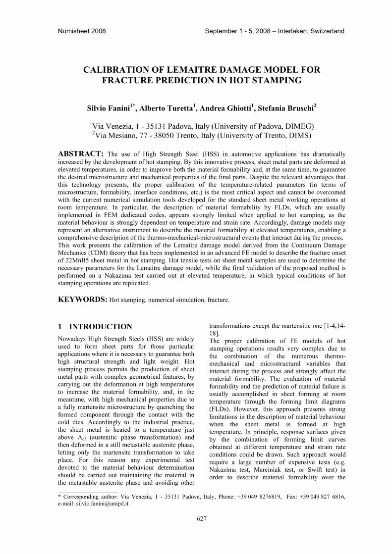
627


____________________* Corresponding author: Via Venezia, 1 - 35131 Padova, Italy, Phone: +39 049 8276819, Fax: +39 049 827 6816, e-mail: [email protected]

CaLIBratION OF LeMaItre DaMaGe MODeL FOr FraCtUre preDICtION IN hOt StaMpING

Silvio Fanini1*, alberto turetta1, andrea Ghiotti1, Stefania Bruschi2

1Via Venezia, 1 - 35131 Padova, Italy (University of Padova, DIMEG) 2Via Mesiano, 77 - 38050 Trento, Italy (University of Trento, DIMS)

aBStraCt: The use of High Strength Steel (HSS) in automotive applications has dramatically increased by the development of hot stamping. By this innovative process, sheet metal parts are deformed at elevated temperatures, in order to improve both the material formability and, at the same time, to guarantee the desired microstructure and mechanical properties of the final parts. Despite the relevant advantages that this technology presents, the proper calibration of the temperature-related parameters (in terms of microstructure, formability, interface conditions, etc.) is the most critical aspect and cannot be overcomed with the current numerical simulation tools developed for the standard sheet metal working operations at room temperature. In particular, the description of material formability by FLDs, which are usually implemented in FEM dedicated codes, appears strongly limited when applied to hot stamping, as the material behaviour is strongly dependent on temperature and strain rate. Accordingly, damage models may represent an alternative instrument to describe the material formability at elevated temperatures, enabling a comprehensive description of the thermo-mechanical-microstructural events that interact during the process. This work presents the calibration of the Lemaitre damage model derived from the Continuum Damage Mechanics (CDM) theory that has been implemented in an advanced FE model to describe the fracture onset of 22MnB5 sheet metal in hot stamping. Hot tensile tests on sheet metal samples are used to determine the necessary parameters for the Lemaitre damage model, while the final validation of the proposed method is performed on a Nakazima test carried out at elevated temperature, in which typical conditions of hot stamping operations are replicated.

KeYWOrDS: Hot stamping, numerical simulation, fracture.

1 INtrODUCtIONNowadays High Strength Steels (HSS) are widely used to form sheet parts for those particular applications where it is necessary to guarantee both high structural strength and light weight. Hot stamping process permits the production of sheet metal parts with complex geometrical features, by carrying out the deformation at high temperatures to increase the material formability, and, in the meantime, with high mechanical properties due to a fully martensite microstructure by quenching the formed component through the contact with the cold dies. Accordingly to the industrial practice, the sheet metal is heated to a temperature just above Ac3 (austenitic phase transformation) and then deformed in a still metastable austenite phase, letting only the martensite transformation to take place. For this reason any experimental test devoted to the material behaviour determination should be carried out maintaining the material in the metastable austenite phase and avoiding other

transformations except the martensitic one [1-4,14-18]. The proper calibration of FE models of hot stamping operations results very complex due to the combination of the numerous thermo-mechanical and microstructural variables that interact during the process and strongly affect the material formability. The evaluation of material formability and the prediction of material failure is usually accomplished in sheet forming at room temperature through the forming limit diagrams (FLDs). However, this approach presents strong limitations in the description of material behaviour when the sheet metal is formed at high temperature. In principle, response surfaces given by the combination of forming limit curves obtained at different temperature and strain rate conditions could be drawn. Such approach would require a large number of expensive tests (e.g. Nakazima test, Marciniak test, or Swift test) in order to describe material formability over the

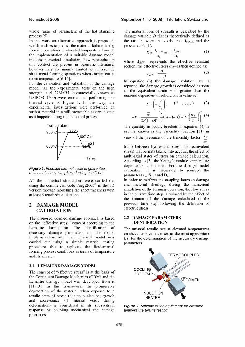
628


whole range of parameters of the hot stamping process [5]. In this work an alternative approach is proposed, which enables to predict the material failure during forming operations at elevated temperature through the implementation of a suitable damage model into the numerical simulation. Few researches in this context are present in scientific literature; however they are mainly limited to analyze the sheet metal forming operations when carried out at room temperature [6-10]. For the calibration and validation of the damage model, all the experimental tests on the high strength steel 22MnB5 (commercially known as USIBOR 1500) were carried out performing the thermal cycle of Figure 1. In this way, the experimental investigations were performed on such a material in a still metastable austenite state as it happens during the industrial process.

Time

Temperature

100°C/s

360 s900°C

600°CTEST

Figure 1: Imposed thermal cycle to guarantee metastable austenite phase testing condition

All the numerical simulations were carried out using the commercial code Forge2005® in the 3D version through modelling the sheet thickness with at least 5 tetrahedron elements.

2 DaMaGe MODeL CaLIBratION

The proposed coupled damage approach is based on the “effective stress” concept according to the Lemaitre formulation. The identification of necessary damage parameters for the model implementation into the numerical model was carried out using a simple material testing procedure able to replicate the fundamental forming process conditions in terms of temperature and strain rate.

2.1 LeMaItre DaMaGe MODeL The concept of “effective stress” is at the basis of the Continuum Damage Mechanics (CDM) and the Lemaitre damage model was developed from it [11-13]. In this framework, the progressive degradation of the material when exposed to a tensile state of stress (due to nucleation, growth and coalescence of internal voids during deformation) is considered in its stress-strain response by coupling mechanical and damage properties.

The material loss of strength is described by the damage variable D that is theoretically defined as the ratio between the voids area AVOIDS and the gross area A0 (1).

00

1A

AA

AD EFFVOIDS (1)

where AEFF represents the effective resistant section; the effective stress EFF is then defined as:

DEFF 1 (2)

In equation (3) the damage evolution law is reported: the damage growth is considered as soon as the equivalent strain is greater than the material dependent threshold strain value th:

s

SYD

0

(if th ) (3)

2

2

2

13132

12H

DEY 2 (4)

The quantity in square brackets in equation (4) is usually known as the triaxiality function [11] in view of the presence of the triaxiality factor H

(ratio between hydrostatic stress and equivalent stress) that permits taking into account the effect of multi-axial states of stress on damage calculation. According to [3], the Young’s module temperature dependence is modelled. For the damage model calibration, it is necessary to identify the parameters th, S0, s and Dc.In order to perform the coupling between damage and material rheology during the numerical simulation of the forming operation, the flow stress in the current time step is reduced by the effect of the amount of the damage calculated at the previous time step following the definition of effective stress.

2.2 DaMaGe paraMeterS IDeNtIFICatION

The uniaxial tensile test at elevated temperatures on sheet samples is chosen as the most appropriate test for the determination of the necessary damage parameters.

COOLING SYSTEM

TERMOCOUPLES

INDUCTION HEATER

SPECIMEN

Figure 2: Scheme of the equipment for elevated temperature tensile testing

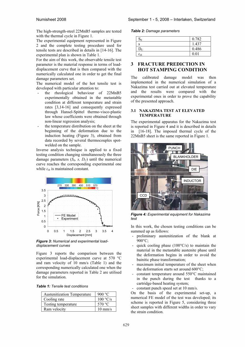
629


The high-strength-steel 22MnB5 samples are tested with the thermal cycle in Figure 1. The experimental equipment represented in Figure 2 and the complete testing procedure used for tensile tests are described in details in [14-16]. The experimental plan is shown in Table 1. For the aim of this work, the observable tensile test parameter is the material response in terms of load-displacement curve that is then compared with the numerically calculated one in order to get the final damage parameters set. The numerical model of the hot tensile test is developed with particular attention to: - the rheological behaviour of 22MnB5

experimentally obtained in the metastable condition at different temperature and strain rates [3,14-16] and consequently expressed through Hansel-Spittel thermo-visco-plastic law whose coefficients were obtained through non-linear regression analysis;

- the temperature distribution on the sheet at the beginning of the deformation due to the induction heating (Figure 3), obtained from data recorded by several thermocouples spot-welded on the sample.

Inverse analysis technique is applied to a fixed testing condition changing simultaneously the three damage parameters (S0, s, DC) until the numerical curve reaches the corresponding experimental one while th is maintained constant.

0

0.5

1

1.5

2

2.5

3

3.5

0 0.5 1 1.5 2 2.5 3 3.5Displacement [mm]

Forc

e [K

N]

4

FE ModelExperiment

570510450390330270°C

Figure 3: Numerical and experimental load-displacement curves

Figure 3 reports the comparison between the experimental load-displacement curve at 570 °C and ram velocity of 10 mm/s (Table 1) and the corresponding numerically calculated one when the damage parameters reported in Table 2 are utilised for the simulation.

Table 1: Tensile test conditions

Austenitization Temperature 900 °C Cooling rate 100 °C/s Testing temperature 570 °C Ram velocity 10 mm/s

Table 2: Damage parameters

S0 0.782 s 1.437 DC 0.486

th 0.01

3 FraCtUre preDICtION IN hOt StaMpING CONDItION

The calibrated damage model was then implemented in the numerical simulation of a Nakazima test carried out at elevated temperature and the results were compared with the experimental ones in order to prove the capability of the presented approach.

3.1 NaKaZIMa teSt at eLeVateD teMperatUre

The experimental apparatus for the Nakazima test is reported in Figure 4 and it is described in details in [16-18]. The imposed thermal cycle of the 22MnB5 sheet is the same reported in Figure 1.

INDUCTOR

PUNCH

CCD

BLANKHOLDER

DIE

Figure 4: Experimental equipment for Nakazima test

In this work, the chosen testing conditions can be summed up as follows: - preliminary austenitization of the blank at

900°C; - quick cooling phase (100°C/s) to maintain the

material in the metastable austenite phase until the deformation begins in order to avoid the bainitic phase transformation;

- maximum initial temperature of the sheet when the deformation starts set around 600°C;

- constant temperature around 550°C maintained in the punch during the test thanks to a cartridge-based heating system;

- constant punch speed set at 10 mm/s. On the basis of the experimental set-up, a numerical FE model of the test was developed; its scheme is reported in Figure 5, considering three sheet samples with different widths in order to vary the strain condition.

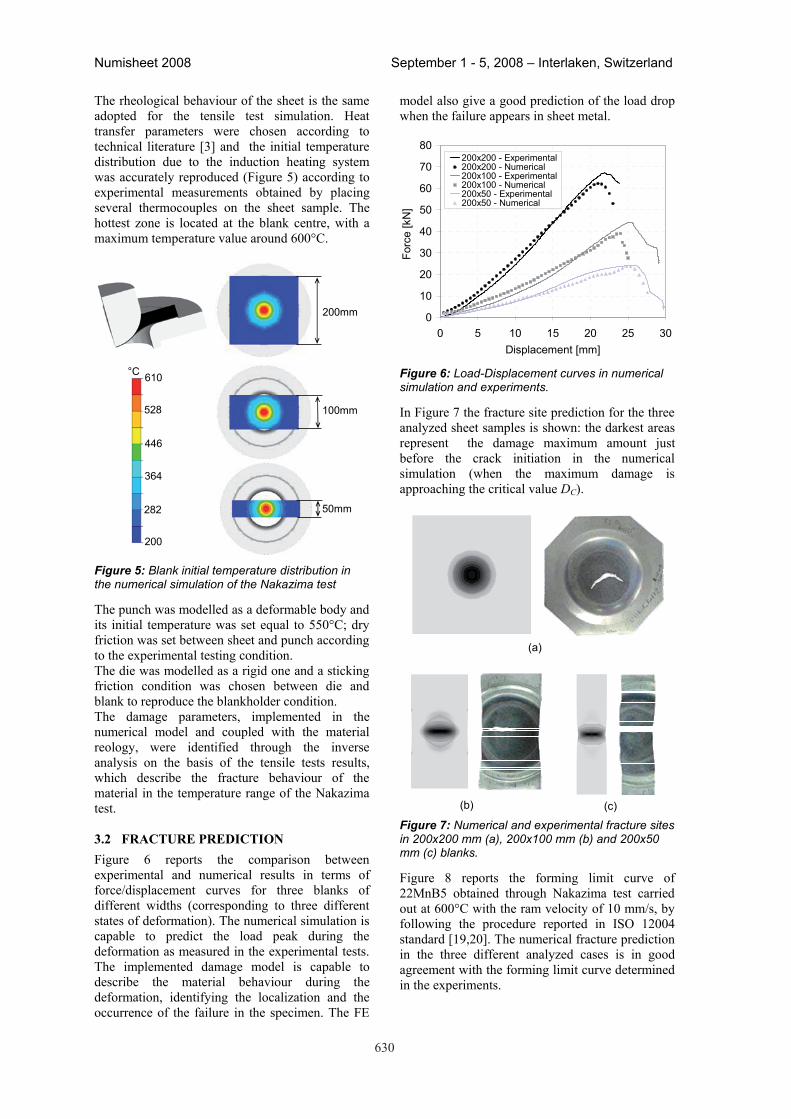
630


The rheological behaviour of the sheet is the same adopted for the tensile test simulation. Heat transfer parameters were chosen according to technical literature [3] and the initial temperature distribution due to the induction heating system was accurately reproduced (Figure 5) according to experimental measurements obtained by placing several thermocouples on the sheet sample. The hottest zone is located at the blank centre, with a maximum temperature value around 600°C.

610

528

446

364

282

200

°C

50mm

100mm

200mm

Figure 5: Blank initial temperature distribution in the numerical simulation of the Nakazima test

The punch was modelled as a deformable body and its initial temperature was set equal to 550°C; dry friction was set between sheet and punch according to the experimental testing condition. The die was modelled as a rigid one and a sticking friction condition was chosen between die and blank to reproduce the blankholder condition. The damage parameters, implemented in the numerical model and coupled with the material reology, were identified through the inverse analysis on the basis of the tensile tests results, which describe the fracture behaviour of the material in the temperature range of the Nakazima test.

3.2 FraCtUre preDICtION Figure 6 reports the comparison between experimental and numerical results in terms of force/displacement curves for three blanks of different widths (corresponding to three different states of deformation). The numerical simulation is capable to predict the load peak during the deformation as measured in the experimental tests. The implemented damage model is capable to describe the material behaviour during the deformation, identifying the localization and the occurrence of the failure in the specimen. The FE

model also give a good prediction of the load drop when the failure appears in sheet metal.

0

10

20

30

40

50

60

70

80

0 5 10 15 20 25 30Displacement [mm]

Forc

e [k

N]

200x200 - Experimental200x200 - Numerical200x100 - Experimental200x100 - Numerical200x50 - Experimental200x50 - Numerical

Figure 6: Load-Displacement curves in numerical simulation and experiments.

In Figure 7 the fracture site prediction for the three analyzed sheet samples is shown: the darkest areas represent the damage maximum amount just before the crack initiation in the numerical simulation (when the maximum damage is approaching the critical value DC).

(a)

(b) (c)

Figure 7: Numerical and experimental fracture sites in 200x200 mm (a), 200x100 mm (b) and 200x50 mm (c) blanks.

Figure 8 reports the forming limit curve of 22MnB5 obtained through Nakazima test carried out at 600°C with the ram velocity of 10 mm/s, by following the procedure reported in ISO 12004 standard [19,20]. The numerical fracture prediction in the three different analyzed cases is in good agreement with the forming limit curve determined in the experiments.

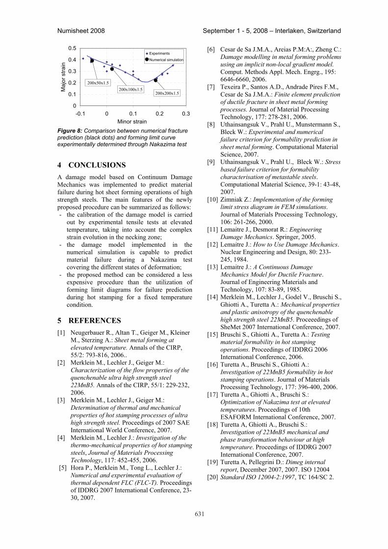
631


0

0.1

0.2

0.3

0.4

0.5

-0.1 0 0.1 0.2 0.3Minor strain

Maj

or s

train

ISO 12004

200x50x1.5

200x200x1.5200x100x1.5

Experiments

Numerical simulation

[6] Cesar de Sa J.M.A., Areias P.M:A:, Zheng C.: Damage modelling in metal forming problems using an implicit non-local gradient model.Comput. Methods Appl. Mech. Engrg., 195: 6646-6660, 2006.

[7] Texeira P., Santos A.D., Andrade Pires F.M., Cesar de Sa J.M.A.: Finite element prediction of ductile fracture in sheet metal forming processes. Journal of Material Processing Technology, 177: 278-281, 2006.

[8] Uthainsangsuk V., Prahl U., Munstermann S., Bleck W.: Experimental and numerical failure criterion for formability prediction in sheet metal forming. Computational Material Science, 2007.

Figure 8: Comparison between numerical fracture prediction (black dots) and forming limit curve experimentally determined through Nakazima test

[9] Uthainsangsuk V., Prahl U., Bleck W.: Stress based failure criterion for formability characterisation of metastable steels.Computational Material Science, 39-1: 43-48, 2007.

4 CONCLUSIONS A damage model based on Continuum Damage Mechanics was implemented to predict material failure during hot sheet forming operations of high strength steels. The main features of the newly proposed procedure can be summarized as follows:

[10] Zimniak Z.: Implementation of the forming limit stress diagram in FEM simulations.Journal of Materials Processing Technology, 106: 261-266, 2000.

- the calibration of the damage model is carried out by experimental tensile tests at elevated temperature, taking into account the complex strain evolution in the necking zone;

[11] Lemaitre J., Desmorat R.: Engineering Damage Mechanics. Springer, 2005.

[12] Lemaitre J.: How to Use Damage Mechanics.Nuclear Engineering and Design, 80: 233-245, 1984.

- the damage model implemented in the numerical simulation is capable to predict material failure during a Nakazima test covering the different states of deformation; [13] Lemaitre J.: A Continuous Damage

Mechanics Model for Ductile Fracture.Journal of Engineering Materials and Technology, 107: 83-89, 1985.

- the proposed method can be considered a less expensive procedure than the utilization of forming limit diagrams for failure prediction during hot stamping for a fixed temperature condition.

[14] Merklein M., Lechler J., Godel V., Bruschi S., Ghiotti A., Turetta A.: Mechanical properties and plastic anisotropy of the quenchenable high strength steel 22MnB5. Proceeedings of SheMet 2007 International Conference, 2007.

5 reFereNCeS [1] Neugerbauer R., Altan T., Geiger M., Kleiner

M., Sterzing A.: Sheet metal forming at elevated temperature. Annals of the CIRP, 55/2: 793-816, 2006..

[15] Bruschi S., Ghiotti A., Turetta A.: Testing material formability in hot stamping operations. Proceedings of IDDRG 2006 International Conference, 2006.

[2] Merklein M., Lechler J., Geiger M.: Characterization of the flow properties of the quenchenable ultra high strength steel 22MnB5. Annals of the CIRP, 55/1: 229-232, 2006.

[16] Turetta A., Bruschi S., Ghiotti A.: Investigation of 22MnB5 formability in hot stamping operations. Journal of Materials Processing Technology, 177: 396-400, 2006.

[17] Turetta A., Ghiotti A., Bruschi S.: Optimization of Nakazima test at elevated temperatures. Proceedings of 10th ESAFORM International Conference, 2007.

[3] Merklein M., Lechler J., Geiger M.: Determination of thermal and mechanical properties of hot stamping processes of ultra high strength steel. Proceedings of 2007 SAE International World Conference, 2007.

[18] Turetta A, Ghiotti A., Bruschi S.: Investigation of 22MnB5 mechanical and phase transformation behaviour at high temperature. Proceedings of IDDRG 2007 International Conference, 2007.

[4] Merklein M., Lechler J.: Investigation of the thermo-mechanical properties of hot stamping steels, Journal of Materials Processing Technology, 117: 452-455, 2006. [19] Turetta A, Pellegrini D.: Dimeg internal

report, December 2007, 2007. ISO 12004 [5] Hora P., Merklein M., Tong L., Lechler J.: Numerical and experimental evaluation of thermal dependent FLC (FLC-T). Proceedings of IDDRG 2007 International Conference, 23-30, 2007.

[20] Standard ISO 12004-2:1997, TC 164/SC 2.

633


DETERMINATION OF FLOW CURVES BY STACKCOMPRESSION TESTS AND INVERSE ANALYSIS FOR THE

SIMULATION OF PRESS HARDENING

B. Hochholdinger1∗, H. Grass2, A. Lipp2, A. Wahlen1, P. Hora1

1 Institute of Virtual Manufacturing, ETH Zurich, 8092 Zurich, Switzerland2 BMW AG, 80788 Munich, Germany

ABSTRACT: Due to the increasing number of body-in-white parts that are manufactured by press hard-ening of boron alloyed sheet metal (22MnB5), the demand for an virtual representation of this specific manu-facturing process is evident. For a realistic simulation of hot stamping processes, the accurate modeling of theflow stress as function of strain, strain rate and temperature is essential.In the last years a large varity of empirical-analytical as well as physically based models for the yield stress hasbeen proposed. Three existing models, that in recent publications have shown a good capability to representthe flow behavior of 22MnB5 are presented and fitted to the experimental data. The underlying experimentaldata for the determination of the flow stress is obtained by stack compression tests. Since in compressiontests the friction between anvil and specimen can have an significant influence on the state of stress within thespecimen, an inverse, simulation-based approach for the determination of the model parameters is presented.

KEYWORDS: flow stress, 22MnB5, press hardening, stack compression test, parameter identification,inverse modeling

1 INTRODUCTIONPress hardening of sheet metal for the productionof ultra high strength structural steel parts is a wellestablished process in the automotive industry to-day. The permanent demand for weight reductionand improved crash performance of the body-in-white will most likely lead to a even higher fractionof crash relevant structural parts, that are manufac-tured by the press hardening process. Due to the factthat press hardening is regarding cycle times, energyconsumption, cooling of the tools, etc. compared toclassical cold forming an expensive process, it is es-sential that the process and tool layout are done vir-tually prior to money and time consuming real try-out loops. In contrast to cold sheet metal formingpress hardening can not be considered isothermal,which means that the temperature field must not beneglected in the simulation and therefore a thermo-mechanically coupled solution strategy has to be fol-lowed.For the coupled IBVP (Initial Boundary Value Prob-lem) the simulation engineer has to define not onlymechanical and thermal initial and boundary con-ditions but also the temperature dependency of the

∗Corresponding author: postal address: Institute of Vir-tual Manufacturing, ETH Zurich, Tannenstrasse 3, 8092 Zurich,Switzerland; phone: +41-44-6322609; fax: +41-44-6321165;email address: [email protected].

mechanical parameters, as e.g. for the friction andthe yield stress. Especially for the direct presshardening process, where the blank is formed andquenchend simultaneously within one process step,the definition of the flow stress as a function depend-ing not only on the strain but also on the strain rateand the temperature is essential in order to achievereliable results.In the subsequent chapters the experimental pro-cedure for the determination of the strain, strainrate and temperature dependency of the yield stressis presented. Furthermore different mathematicalmodels are fitted to the experimental results and thecapability of the models to reproduce the test data iscompared. In order to account for the influence offriction on the test results, an inverse, simulation-based method to identify the model parameters ispresented.

2 MATERIAL PROPERTIES ANDEXPERIMENTAL SETUP

The material examined is phs-ultraform R�, whichis the trade name for steel grade 22MnB5 fromvoestalpine AG. The experiments for the deter-mination of the plastic flow properties were con-ducted in a high-speed deformation dilatometer“Bahr DIL805A/D” by upsetting tests.Currently 22MnB5 is more or less the only steel

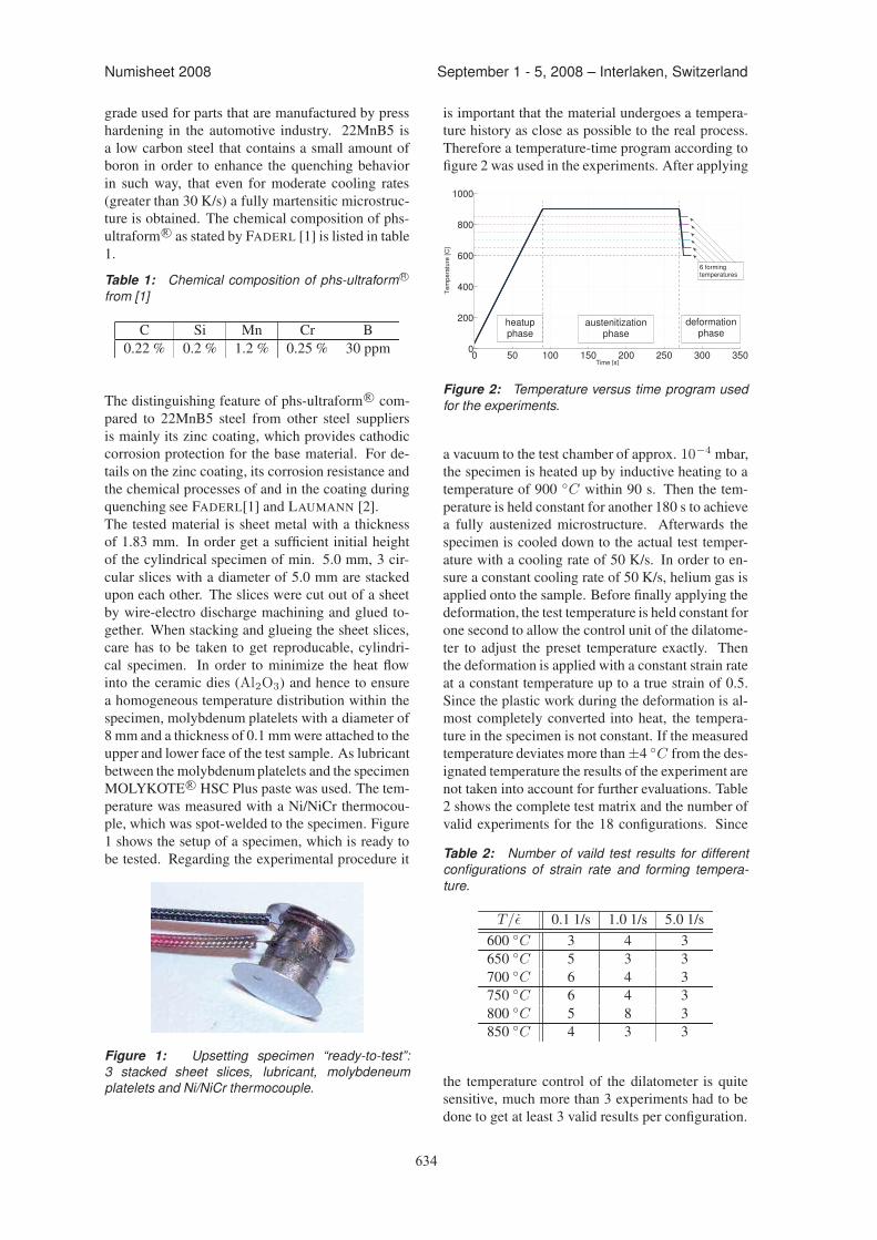
634


grade used for parts that are manufactured by presshardening in the automotive industry. 22MnB5 isa low carbon steel that contains a small amount ofboron in order to enhance the quenching behaviorin such way, that even for moderate cooling rates(greater than 30 K/s) a fully martensitic microstruc-ture is obtained. The chemical composition of phs-ultraform R� as stated by FADERL [1] is listed in table1.

Table 1: Chemical composition of phs-ultraform R�

from [1]

C Si Mn Cr B0.22 % 0.2 % 1.2 % 0.25 % 30 ppm

The distinguishing feature of phs-ultraform R� com-pared to 22MnB5 steel from other steel suppliersis mainly its zinc coating, which provides cathodiccorrosion protection for the base material. For de-tails on the zinc coating, its corrosion resistance andthe chemical processes of and in the coating duringquenching see FADERL[1] and LAUMANN [2].The tested material is sheet metal with a thicknessof 1.83 mm. In order get a sufficient initial heightof the cylindrical specimen of min. 5.0 mm, 3 cir-cular slices with a diameter of 5.0 mm are stackedupon each other. The slices were cut out of a sheetby wire-electro discharge machining and glued to-gether. When stacking and glueing the sheet slices,care has to be taken to get reproducable, cylindri-cal specimen. In order to minimize the heat flowinto the ceramic dies (Al2O3) and hence to ensurea homogeneous temperature distribution within thespecimen, molybdenum platelets with a diameter of8 mm and a thickness of 0.1 mmwere attached to theupper and lower face of the test sample. As lubricantbetween the molybdenumplatelets and the specimenMOLYKOTE R� HSC Plus paste was used. The tem-perature was measured with a Ni/NiCr thermocou-ple, which was spot-welded to the specimen. Figure1 shows the setup of a specimen, which is ready tobe tested. Regarding the experimental procedure it

Figure 1: Upsetting specimen “ready-to-test”:3 stacked sheet slices, lubricant, molybdeneumplatelets and Ni/NiCr thermocouple.

is important that the material undergoes a tempera-ture history as close as possible to the real process.Therefore a temperature-time program according tofigure 2 was used in the experiments. After applying

0 50 100 150 200 250 300 3500

200

400

600

800

1000

Time [s]

Tem

pera

ture

[C]

6 formingtemperatures

austenitizationphase

deformationphase

heatupphase

Figure 2: Temperature versus time program usedfor the experiments.

a vacuum to the test chamber of approx. 10−4 mbar,the specimen is heated up by inductive heating to atemperature of 900 ◦C within 90 s. Then the tem-perature is held constant for another 180 s to achievea fully austenized microstructure. Afterwards thespecimen is cooled down to the actual test temper-ature with a cooling rate of 50 K/s. In order to en-sure a constant cooling rate of 50 K/s, helium gas isapplied onto the sample. Before finally applying thedeformation, the test temperature is held constant forone second to allow the control unit of the dilatome-ter to adjust the preset temperature exactly. Thenthe deformation is applied with a constant strain rateat a constant temperature up to a true strain of 0.5.Since the plastic work during the deformation is al-most completely converted into heat, the tempera-ture in the specimen is not constant. If the measuredtemperature deviates more than±4 ◦C from the des-ignated temperature the results of the experiment arenot taken into account for further evaluations. Table2 shows the complete test matrix and the number ofvalid experiments for the 18 configurations. Since

Table 2: Number of vaild test results for differentconfigurations of strain rate and forming tempera-ture.

T/� 0.1 1/s 1.0 1/s 5.0 1/s600 ◦C 3 4 3650 ◦C 5 3 3700 ◦C 6 4 3750 ◦C 6 4 3800 ◦C 5 8 3850 ◦C 4 3 3

the temperature control of the dilatometer is quitesensitive, much more than 3 experiments had to bedone to get at least 3 valid results per configuration.

635


3 EXPERIMENTAL RESULTSFigure 3 shows exemplarily the experimental re-sults for strain rate 1.0 1/s for test temperaturesT = 650, 750 and 850 ◦C, respectively. Foreach test configuration the individual curves of the“valid” experiments (thin line) as well as the aver-aged curve (thick line) are displayed. Accordingly,in figure 4 the experimental results for the strainrates � = 0.05, 0.1, 1.0 and 5.0 1/s at a testtemperature of T = 650 ◦C are displayed. Theoscillations within the individual stress curves aremainly due to fluctuations of the temperature duringthe compression of the specimen.

0 0.1 0.2 0.3 0.4 0.50

100

200

300

400

500

εp [−]

σ y [MPa

]

750 C 850 C

650 C

Figure 3: Flow stress curves for 3 test temperaturesat a constant strain rate � = 1.0 1/s.

0 0.1 0.2 0.3 0.4 0.50

100

200

300

400

500

εp [−]

σ y [MPa

]

5.0 1/s

0.1 1/s1.0 1/s

Figure 4: Flow stress curves for 3 strain rates at aconstant test temperature T = 650

◦C.

4 MATHEMATICAL MODELINGDuring the last years several papers have been pub-lished presenting different models for the flow stressof 22MnB5 as a function of strain, strain rate andtemperature. The experimental results were eitherobtained by hot tension tests as for example in BRO-

SIUS [3] and MERKLEIN [4] or by compression testsusing conventional (ERIKSSON [5], NADERI [6]) orstacked specimens (BURKHARDT [7]).According to BARIANI [8] one can generally distin-guish between empirical anlytical, physically-basedand empirical non-analytical models. Empirical an-alytical models deploy phenomenological derivedexpressions to model the flow stress as a functionof macroscopic process parameters. The materialconstants within such formulations do not have aphysical meaning and are usually determined by re-gression analysis. In contrast to empirical analyticalmodels, the so-called physically-based models arefunctions of internal variables, which reflect the ini-tial physical (micro-)structure of the material as wellas its evolution. Empirical non-analytical models,which use instead of an explicit analytical expres-sion for the flow stress usually a neural network-based approach, are not considered in this paper.For practical applications empirical analytical mod-els – due to their simplicity – are often favored overphysically-based models. The later require complexand expensive experiments to determine the internalvariables with an adequate accuracy. It is also popu-lar to use a combination of both approaches. Whenfor such models the parameters are fitted to the ex-perimental data, the resulting values for the parame-ters with a physical meaning can be checked versusvalues from literature. This provides a first checkregarding the validity of the model and/or the fittingprocedure, respectively. In this paper three models,which have shown a good capability to reproducethe experimental data for 22MnB5, have been se-lected and evaluated.

4.1 NORTON-HOFFMODELThe first model considered is a modified Norton-Hoff approach as described in BROSIUS [3]. Asin most models, that follow the empirical-analyticalapproach, the components that account for thestrain-, strain rate- and temperaturedependency ofthe flow stress are multiplied with each other. Theoriginal NORTON-HOFF model has the followingform.

σy(�p, �p, T ) = K� ·K� ·KT = K�np · �mp · eβ

T (1)

In order to correctly reproduce the initial yield stressand to account for the temperature dependency ofK� andK� equation 1 has been extended by definingparameters n andm as a function of temperature T ,respectively (see equation 2 as defined in [3]).

σy(�p, �p, T ) = K (b + �p)n(T )

· �m(T )p · e

β

T

with n(T ) = n0 · e−cn(Ti−T0) (2)

and m(T ) = m0 · ecm(Ti−T0)

Consequently 7 parameters (K , b, n0, cn, m0, cm,β) have to be determined in order to approximate the

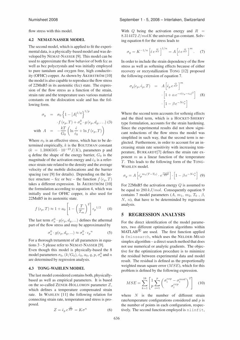
636


flow stress with this model.

4.2 NEMAT-NASSER MODELThe second model, which is applied to fit the experi-mental data, is a physically-basedmodel and was de-veloped by NEMAT-NASSER [9]. This model can beused to approximate the flow behavior of both fcc aswell as bcc polycrystals and was initially employedto pure tantalum and oxygen free, high conductiv-ity (OFHC) copper. As shown by AKERSTROM [10]the model is also capable to reproduce the flow stressof 22MnB5 in its austenitic (fcc) state. The expres-sion of the flow stress as a function of the strain,strain rate and the temperature uses various materialconstants on the dislocation scale and has the fol-lowing form.

σy = σ0

�

1 − [A]1/q

�1/p

·f (�p, T ) + σ0a · g (�p, dg, . . .) (3)

with A = −kT

G0

�

ln�

�0+ ln f (�p, T )

�

Where σ0 is an effective stress, which has to be de-termined empirically, k is the BOLTZMAN constant(k = 1.3806505 · 10−23J/K), parameters p andq define the shape of the energy barrier, G0 is themagnitude of the activation energy and �0 is a refer-ence strain rate related to the density and the averagevelocity of the mobile dislocations and the barrierspacing (see [9] for details). Depending on the lat-tice structure – fcc or bcc – the function f (�p, T )takes a different expression. In AKERSTROM [10]the formulation according to equation 4, which wasinitially used for OFHC copper, is also used for22MnB5 in its austenitic state.

f (�p, T ) ≈ 1 + a0

�

1 −

�

T

Tm

�2�

�p1/2 (4)

The last term σ0a · g(�p, dg, ...) defines the athermal

part of the flow stress and may be approximated by

σ0a · g(�p, dg, ...) ≈ σ0

a · �pn (5)

For a thorough tretamtent of all parameters in equa-tions 3 - 5 please refer to NEMAT-NASSER [9].Even though this model is physically-based the 8model parameters σ0, (k/G0), �0, a0, q, p, σ0

a and nare determined by regression analysis.

4.3 TONG-WAHLENMODELThe last model considered contains both, physically-based as well as empirical parameters. It is basedon the so-called ZENER-HOLLOMON parameter Z,which defines a temperature compensated strainrate. In WAHLEN [11] the following relation forconnecting strain rate, temperature and stress is pro-posed.

Z = �p eQ

RT = Kσn (6)

With Q being the activation energy and R =8.314472 J/molK the universal gas constant. Solv-ing equation 6 for the stress leads to

σy = K−1/n�

� eQ

RT

�1/n

= A�

� eQ

RT

�m

. (7)

In order to include the strain dependency of the flowstress as well as softening effects because of eitherrecovery or recrystallization TONG [12] proposedthe following extension of equation 7.

σy(�p, �p, T ) = A�

�p eQ

RT

�m

·

�

1 + α e−c(�p−�0)2�

(8)

·

�

1 − β e−N�np

�

Where the second term accounts for softenig effectsand the third term, which is a HOCKET-SHERBYtype formulation, accounts for the strain hardening.Since the experimental results did not show signi-cant reductions of the flow stress the model wassimplified in such way, that the second term is ne-glected. Furthermore, in order to account for an in-creasing strain rate sensitivity with increasing tem-perature, BURKARDT[7] defines the strain rate ex-ponent m as a linear function of the temperatureT . This leads to the following form of the TONG-WAHLEN model.

σy = A�

�pm1(T−T0)

· em2Q

RT

�

·

�

1 − β e−N�np

�

(9)

For 22MnB5 the activation energy Q is assumed tobe equal to 280 kJ/mol. Consequently equation 9contains 7 model parameters (A, m1, m2, T0 , β,N , n), that have to be determinded by regressionanalysis.

5 REGRESSION ANALYSISFor the direct identification of the model parame-ters, two different optimization algorithms withinMATLAB R� are used. The first function appliedis fminsearch, which uses the NELDER-MEADsimplex algorithm – a direct search method that doesnot use numerical or analytic gradients. The objec-tive for the optimization procedure is to minimizethe residual between experimental data and modelresult. The residual is defined as the proportionallyweighted mean square error (MSE), which for thisproblem is defined by the following expression.

MSE =

18�

k=1

�

1

p

p�

i=1

�

σexpi − σmod

i

σexpi

�2�

(10)

where N is the number of different strainrate/temperature configurations considered and p isthe number of points in each configuration, respec-tively. The second function employed is nlinfit,

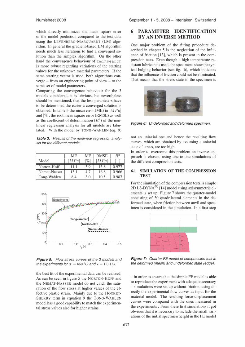
637


which directly minimizes the mean square errorof the model prediction compared to the test datausing the LEVENBERG-MARQUARDT (LM) algo-rithm. In general the gradient-based LM algorithmneeds much less iterations to find a converged so-lution than the simplex algorithm. On the otherhand the convergence behaviour of fminsearchis more robust regarding variations of the startingvalues for the unknown material parameters. If thesame starting vector is used, both algorithms con-verge – from an engineering point of view – to thesame set of model parameters.Comparing the convergence behaviour for the 3models considered, it is obvious, but neverthelessshould be mentioned, that the less parameters haveto be determined the easier a converged solution isobtained. In table 3 the mean error (ME) in [MPa]and [%], the root mean square error (RMSE) as wellas the coefficient of determination (R2) of the non-linear regression analysis for all models are tabu-lated. With the model by TONG-WAHLEN (eq. 9)

Table 3: Results of the nonlinear regression analy-sis for the different models.

ME ME RMSE R2

Model [MPa] [%] [MPa] [−]

Norton-Hoff 11.1 3.9 13.8 0.977Nemat-Nasser 13.1 4.7 16.8 0.966Tong-Wahlen 8.4 3.0 10.5 0.987

0 0.1 0.2 0.3 0.4 0.50

100

200

300

400

500

εp [−]

σ y [MPa

]

Norton−HoffTong−Wahlen

Experiments

Nemat−Nasser

Figure 5: Flow stress curves of the 3 models andthe experiments for T = 650

◦C and � = 1.0 1/s.

the best fit of the experimental data can be realized.As can be seen in figure 5 the NORTON-HOFF andthe NEMAT-NASSER model do not catch the satu-ration of the flow stress at higher values of the ef-fective plastic strain. Mainly due to the HOCKET-SHERBY term in equation 9 the TONG-WAHLENmodel has a good capability to match the experimen-tal stress values also for higher strains.

6 PARAMETER IDENTIFICATIONBY AN INVERSE METHOD

One major problem of the fitting procedure de-scribed in chapter 5 is the neglection of the influ-ence of friction [13], which is present in the com-pression tests. Even though a high temperature re-sistant lubricant is used, the specimens show the typ-ical bulging behavior (see fig. 6), which indicatesthat the influence of friction could not be eliminated.That means that the stress state in the specimen is

Figure 6: Undeformed and deformed specimen.

not an uniaxial one and hence the resulting flowcurves, which are obtained by assuming a uniaxialstate of stress, are too high.In order to overcome this problem an inverse ap-proach is chosen, using one-to-one simulations ofthe different compression tests.

6.1 SIMULATION OF THE COMPRESSIONTEST

For the simulation of the compression tests, a simple2D LS-DYNA R� [14] model using axisymmetric el-ements is set up. Figure 7 shows the quarter-modelconsisting of 30 quadrilateral elements in the de-formed state, when friction between anvil and spec-imen is considered in the simulation. In a first step

Figure 7: Quarter FE model of compression test inthe deformed (mesh) and undeformed state (edge).

– in order to ensure that the simple FE model is ableto reproduce the experiment with adequate accuracy– simulations were set up without friction, using di-rectly the experimental flow curves as input for thematerial model. The resulting force-displacementcurves were compared with the ones measured inthe experiments . From these first simulations it gotobvious that it is necessary to include the small vari-ations of the initial specimen height in the FE model

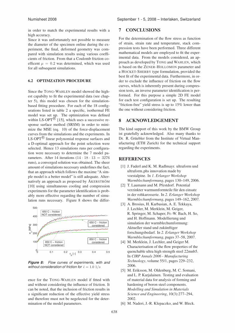
638


in order to match the experimental results with ahigh accuracy.Since it was unfortunately not possible to measurethe diameter of the specimen online during the ex-periment, the final, deformed geometry was com-pared with simulation results using various coeffi-cients of friction. From that a Coulomb friction co-efficent µ = 0.2 was determined, which was usedfor all subsequent simulations.

6.2 OPTIMZATION PROCEDURE

Since the TONG-WAHLEN model showed the high-est capabilty to fit the experimental data (see chap-ter 5), this model was chosen for the simulation-based fitting procedure. For each of the 18 config-urations listed in table 2 a specific, isothermal FEmodel was set up. The optimization was definedwithin LS-OPT R� [15], which uses a successive re-sponse surface method (SRSM) in order to mini-mize the MSE (eq. 10) of the force-displacementcurves from the simulations and the experiments. InLS-OPT R� linear polynomial response surfaces anda D-optimal approach for the point selection wereselected. Hence 13 simulations runs per configura-tion were necessary to determine the 7 model pa-rameters. After 14 iterations (14 · 18 · 13 = 3276runs), a converged solution was obtained. The sheeramount of simulations necessary underlines the fact,that an approach which follows the maxime “A sim-ple model is a better model” is still adequate. Alter-natively an approach as proposed by AKERSTROM[10] using simultaneous cooling and compressionexperiments for the parameter identification is prob-ably more effective regarding the number of simu-lation runs necessary. Figure 8 shows the differ-

0 0.1 0.2 0.3 0.4 0.50

100

200

300

400

500

εp [−]

σ y [MPa

]

850 C − frictionNOT considered

650 C − frictionconsidered

850 C − frictionconsidered

650 C − frictionNOT considered

Figure 8: Flow curves of experiments, with andwithout consideration of friction for � = 1.0 1/s

ence for the TONG-WAHLEN model if fitted withand without considering the influence of friction. Itcan be noted, that the inclusion of friction results ina significant reduction of the effective yield stressand therefore must not be negelected for the deter-mination of the model parameters.

7 CONCLUSIONSFor the determination of the flow stress as functionof strain, strain rate and temperature, stack com-pression tests have been performed. Three differentmathematical models are employed to fit the exper-imental data. From the models considered, an ap-proach as developed by TONG and WAHLEN, whichis based on the ZENER-HOLLOMON parameter anda HOCKET-SHERBY type formulation, provided thebest fit of the experimental data. Furthermore, in or-der to exclude the influence of friction on the flowcurves, which is inherently present during compres-sion tests, an inverse parameter identification is per-formed. For this purpose a simple 2D FE modelfor each test configuration is set up. The resulting“friction-free” yield stress is up to 15% lower thanthe one without considering friction.

8 ACKNOWLEDGEMENTThe kind support of this work by the BMW Groupist gratefully acknowledged. Also many thanks toDr. R. Gruebler from the Institute of Virtual Man-ufacturing (ETH Zurich) for the technical supportregarding the experiments.

REFERENCES[1] J. Faderl and K. M. Radlmayr. ultraform und

ultraform phs innovation made byvoestalpine. In 1. Erlanger WorkshopWarmblechumformung, pages 130–149, 2006.

[2] T. Laumann and M. Pfestdorf. Potentialverzinkter warmumformteile fur den einsatzin der rohkarosserie. In 2. Erlanger WorkshopWarmblechumformung, pages 149–162, 2007.

[3] A. Brosius, H. Karbasian, A. E. Tekkaya,J. Lechler, M. Merklein, M. Geiger,R. Springer, M. Schaper, Fr.-W. Bach, H. So,and H. Hoffmann. Modellierung undsimulation der warmblechumformung:Aktueller stand und zukunftigerforschungsbedarf. In 2. Erlanger WorkshopWarmblechumformung, pages 37–58, 2007.

[4] M. Merklein, J. Lechler, and Geiger M.Characterisation of the flow properties of thequenchable ultra high strength steel 22mnb5.In CIRP Annals 2006 - ManufacturingTechnology, volume 55/1, pages 229–232,2006.

[5] M. Eriksson, M. Oldenburg, M. C. Somani,and L. P. Karjalainen. Testing and evaluationof material data for analysis of forming andhardening of boron steel components.Modelling and Simulation in MaterialsScience and Engineering, 10(3):277–294,2002.

[6] M. Naderi, J.-R. Klepaczko, and W. Bleck.

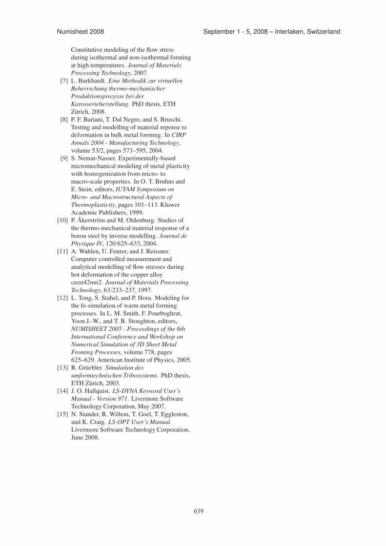
639


Constitutive modeling of the flow stressduring isothermal and non-isothermal formingat high temperatures. Journal of MaterialsProcessing Technology, 2007.

[7] L. Burkhardt. Eine Methodik zur virtuellenBeherrschung thermo-mechanischerProduktionsprozesse bei derKarosserieherstellung. PhD thesis, ETHZurich, 2008.

[8] P. F. Bariani, T. Dal Negro, and S. Bruschi.Testing and modelling of material reponse todeformation in bulk metal forming. In CIRPAnnals 2004 - Manufacturing Technology,volume 53/2, pages 573–595, 2004.

[9] S. Nemat-Nasser. Experimentally-basedmicromechanical modeling of metal plasticitywith homogenization from micro- tomacro-scale properties. In O. T. Bruhns andE. Stein, editors, IUTAM Symposium onMicro- and Macrostructural Aspects ofThermoplasticity, pages 101–113. KluwerAcademic Publishers, 1999.

[10] P. Akerstrom and M. Oldenburg. Studies ofthe thermo-mechanical material response of aboron steel by inverse modelling. Journal dePhysique IV, 120:625–633, 2004.

[11] A. Wahlen, U. Feurer, and J. Reissner.Computer controlled measurement andanalytical modelling of flow stresses duringhot deformation of the copper alloycuzn42mn2. Journal of Materials ProcessingTechnology, 63:233–237, 1997.

[12] L. Tong, S. Stahel, and P. Hora. Modeling forthe fe-simulation of warm metal formingprocesses. In L. M. Smith, F. Pourboghrat,Yoon J.-W., and T. B. Stoughton, editors,NUMISHEET 2005 - Proceedings of the 6thInternational Conference and Workshop onNumerical Simulation of 3D Sheet MetalFroming Processes, volume 778, pages625–629. American Institute of Physics, 2005.

[13] R. Gruebler. Simulation desumformtechnischen Tribosystems. PhD thesis,ETH Zurich, 2003.

[14] J. O. Hallquist. LS-DYNA Keyword User’sManual - Version 971. Livermore SoftwareTechnology Corporation, May 2007.

[15] N. Stander, R. Willem, T. Goel, T. Eggleston,and K. Craig. LS-OPT User’s Manual.Livermore Software Technology Corporation,June 2008.

641


TEMPERATURE AND VELOCITY DEPENDENT FRICTIONMODELING FOR SHEET METAL FORMING PROCESSES

R. Grueebler1∗, P. Hora1

1 ETH Zurich, Institute of Virtual Manufacturing (IVP), Switzerland

ABSTRACT: Stainless steels in cold forming processes show a hardening behavior, which can be describedonly in dependency of the deformation and temperature history. Because of the temperature influence on thematerial properties of those steels, the temperature dependence of the friction in the process has to be taken intoaccount. The friction characteristics in stainless steel forming has been examined regarding to the temperatureand velocity influence. Friction tests were performed using different temperatures and velocities. From theexperimental observation the temperature and velocity dependence of the friction was modeled and integratedin a finite element code for metal forming. The FE simulation has been applied to the biaxial stretching testand compared with the experiment. The numerical results showed a good agreement with the failure behaviorof the stainless steel.

KEYWORDS: Friction modeling, FEM simulation, Lubrication

1 INTRODUCTIONIn the manufacturing of stainless sheet metal prod-ucts the processes are optimized regarding the re-quirements for efficiency as well as for quality im-provement and for the augmentation of piece variety.Therefore the process parameters have to be wellknown. An important parameter in the process isthe friction because of the large contact area. Hencethe friction plays a major role in sheet metal formingprocesses.The contact area between the sheet and the form-ing tool, including the lubricating agent, is the mostcomplex part of the tribological system. The pres-ence of an effective lubricant film thickness be-tween contact surfaces in the metal forming pro-cess increases the forming limit, reduces tool wear,and improves the product quality. Different lubri-cation regimes may occur in different areas of theinterface or at different time due to different fac-tors influencing the friction like temperature, normalforce, velocity. Therfore the analysis of the tool-ing/workpiece interface friction with lubrication inmetal forming processes is extremely complicated.Since the strain distribution in the workpiece is influ-enced by friction, the formability of the workpiecedepends not only the material properties but also onthe friction at the tooling/workpiece interface. Thefriction is essential to guarantee the formability ofthe sheet and to improve the accuracy of the com-puter simulation. Because of the temperature influ-

∗Corresponding author: Tannenstr. 3 8092 Zurich, p +41 44632 26 17 f +41 44 632 11 65, [email protected],

ence on the material properties of those steels, thetemperature dependence of the friction in the pro-cess has to be taken into account. The considerationof the temperature dependence in the material prop-erties and friction is important for the formability ofthe stainless sheet metal.There are different approaches to include the depen-dencies of the friction. Keum et al. [1] measuredexperimentally the effects of lubricant viscosity, sur-face roughness and hardness of the sheet, punch ve-locity and die corner radius on the friction. He sug-gested a mathematical model of the friction coeffi-cient as a function of friction parameters. This is anempirical model on the macroscale, which is easyto use in a computer simulation but that does notconsider the physical processes. For a more theoret-ical approach the processes on the microscopic scalehave to be considered. On this scale it is possible todivide the friction in different regimes. Wilson et al.[2] developed a theoretical model of thick film lu-brication for a simple stretch forming process witha cylindrical or spherical punch. This model con-siders no asperity contact at the tooling/workpieceinterfaces. But the boundary friction regime is im-portant in sheet metal forming especially for stain-less steels. The surface texture has an importantinfluence on the friction ([3][4]). A lot of modelsconsider the asperity contact, most of them with thestatic equilibrium solution in pure flattening [5], [6],[7] and [8]. The asperity contact in sliding flatten-ing is more complicated, because of the additionaltangential stress. Lo and Yang [9] proposed a newconcept of asperity flattening. The different friction

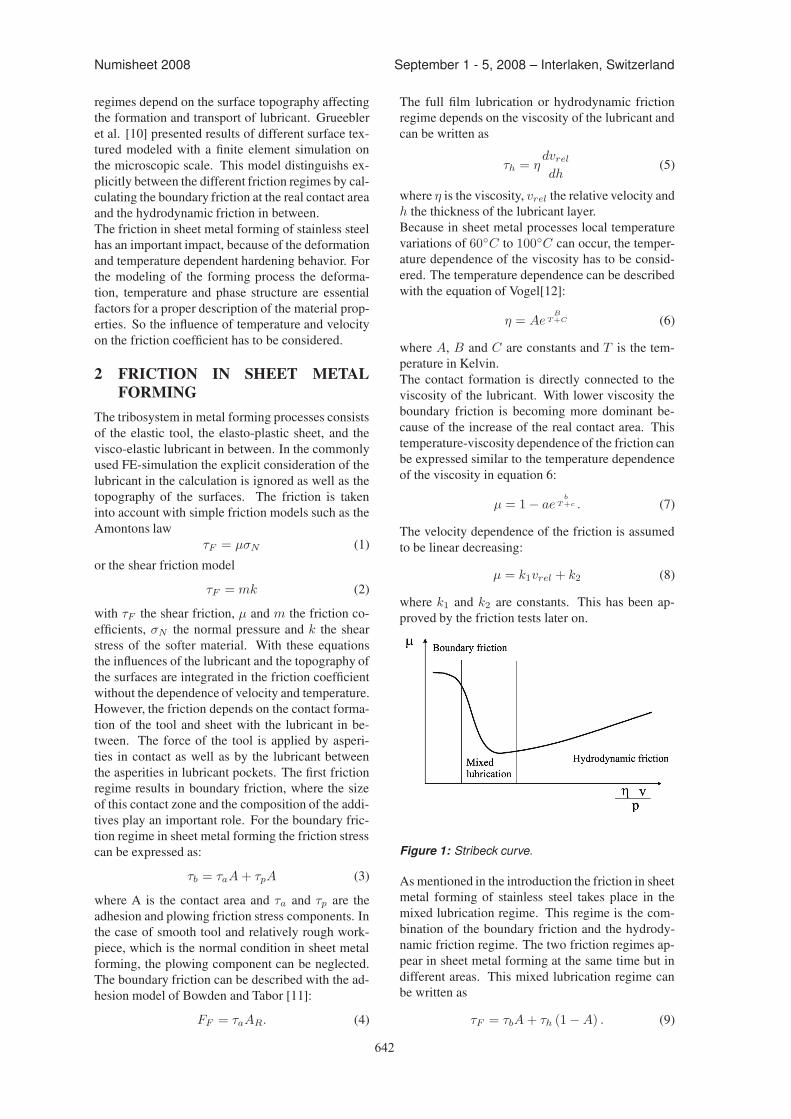
642


regimes depend on the surface topography affectingthe formation and transport of lubricant. Grueebleret al. [10] presented results of different surface tex-tured modeled with a finite element simulation onthe microscopic scale. This model distinguishs ex-plicitly between the different friction regimes by cal-culating the boundary friction at the real contact areaand the hydrodynamic friction in between.The friction in sheet metal forming of stainless steelhas an important impact, because of the deformationand temperature dependent hardening behavior. Forthe modeling of the forming process the deforma-tion, temperature and phase structure are essentialfactors for a proper description of the material prop-erties. So the influence of temperature and velocityon the friction coefficient has to be considered.

2 FRICTION IN SHEET METALFORMING

The tribosystem in metal forming processes consistsof the elastic tool, the elasto-plastic sheet, and thevisco-elastic lubricant in between. In the commonlyused FE-simulation the explicit consideration of thelubricant in the calculation is ignored as well as thetopography of the surfaces. The friction is takeninto account with simple friction models such as theAmontons law

τF = µσN (1)or the shear friction model

τF = mk (2)

with τF the shear friction, µ and m the friction co-efficients, σN the normal pressure and k the shearstress of the softer material. With these equationsthe influences of the lubricant and the topography ofthe surfaces are integrated in the friction coefficientwithout the dependence of velocity and temperature.However, the friction depends on the contact forma-tion of the tool and sheet with the lubricant in be-tween. The force of the tool is applied by asperi-ties in contact as well as by the lubricant betweenthe asperities in lubricant pockets. The first frictionregime results in boundary friction, where the sizeof this contact zone and the composition of the addi-tives play an important role. For the boundary fric-tion regime in sheet metal forming the friction stresscan be expressed as:

τb = τaA + τpA (3)

where A is the contact area and τa and τp are theadhesion and plowing friction stress components. Inthe case of smooth tool and relatively rough work-piece, which is the normal condition in sheet metalforming, the plowing component can be neglected.The boundary friction can be described with the ad-hesion model of Bowden and Tabor [11]:

FF = τaAR. (4)

The full film lubrication or hydrodynamic frictionregime depends on the viscosity of the lubricant andcan be written as

τh = ηdvrel

dh(5)

where η is the viscosity, vrel the relative velocity andh the thickness of the lubricant layer.Because in sheet metal processes local temperaturevariations of 60◦C to 100◦C can occur, the temper-ature dependence of the viscosity has to be consid-ered. The temperature dependence can be describedwith the equation of Vogel[12]:

η = AeB

T+C (6)

where A, B and C are constants and T is the tem-perature in Kelvin.The contact formation is directly connected to theviscosity of the lubricant. With lower viscosity theboundary friction is becoming more dominant be-cause of the increase of the real contact area. Thistemperature-viscosity dependence of the friction canbe expressed similar to the temperature dependenceof the viscosity in equation 6:

µ = 1 − aeb

T+c . (7)

The velocity dependence of the friction is assumedto be linear decreasing:

µ = k1vrel + k2 (8)

where k1 and k2 are constants. This has been ap-proved by the friction tests later on.

Figure 1: Stribeck curve.

Asmentioned in the introduction the friction in sheetmetal forming of stainless steel takes place in themixed lubrication regime. This regime is the com-bination of the boundary friction and the hydrody-namic friction regime. The two friction regimes ap-pear in sheet metal forming at the same time but indifferent areas. This mixed lubrication regime canbe written as

τF = τbA + τh (1 − A) . (9)

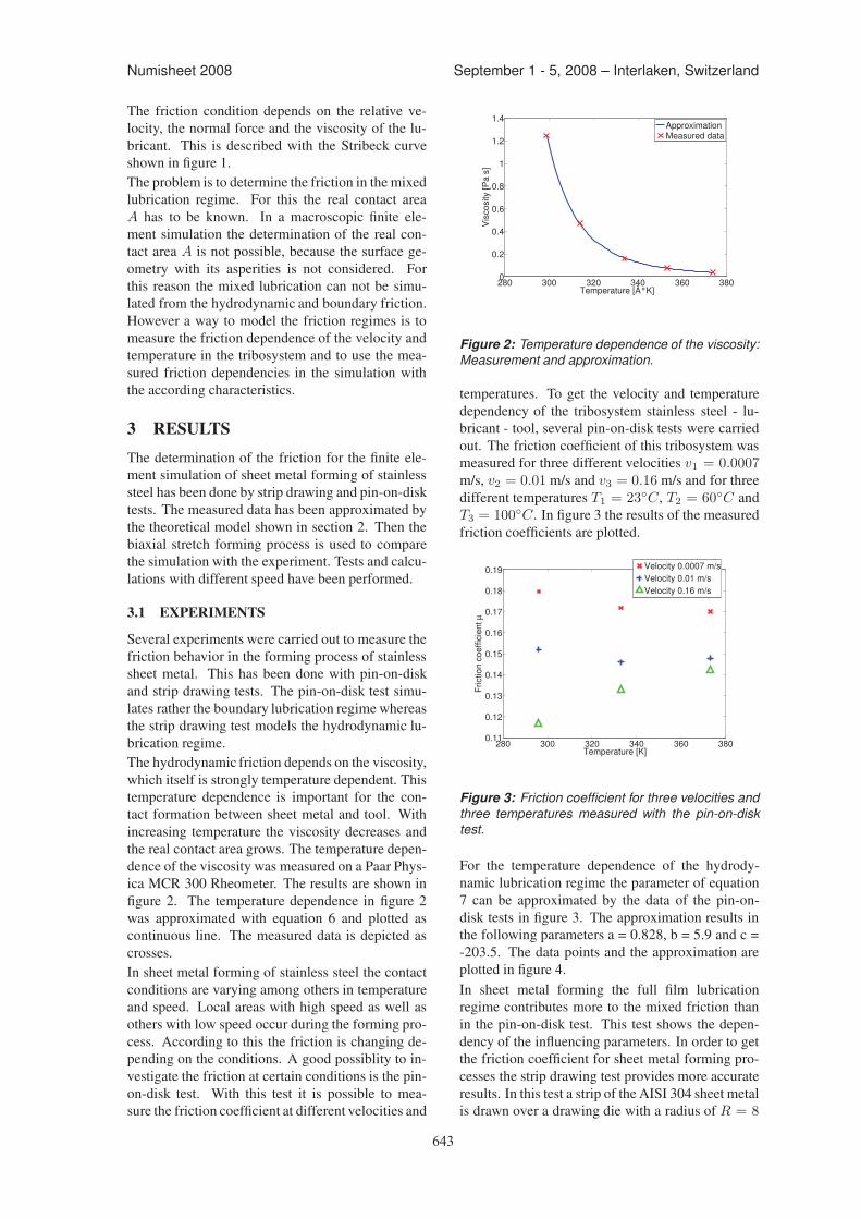
643


The friction condition depends on the relative ve-locity, the normal force and the viscosity of the lu-bricant. This is described with the Stribeck curveshown in figure 1.The problem is to determine the friction in the mixedlubrication regime. For this the real contact areaA has to be known. In a macroscopic finite ele-ment simulation the determination of the real con-tact area A is not possible, because the surface ge-ometry with its asperities is not considered. Forthis reason the mixed lubrication can not be simu-lated from the hydrodynamic and boundary friction.However a way to model the friction regimes is tomeasure the friction dependence of the velocity andtemperature in the tribosystem and to use the mea-sured friction dependencies in the simulation withthe according characteristics.

3 RESULTSThe determination of the friction for the finite ele-ment simulation of sheet metal forming of stainlesssteel has been done by strip drawing and pin-on-disktests. The measured data has been approximated bythe theoretical model shown in section 2. Then thebiaxial stretch forming process is used to comparethe simulation with the experiment. Tests and calcu-lations with different speed have been performed.

3.1 EXPERIMENTSSeveral experiments were carried out to measure thefriction behavior in the forming process of stainlesssheet metal. This has been done with pin-on-diskand strip drawing tests. The pin-on-disk test simu-lates rather the boundary lubrication regime whereasthe strip drawing test models the hydrodynamic lu-brication regime.The hydrodynamic friction depends on the viscosity,which itself is strongly temperature dependent. Thistemperature dependence is important for the con-tact formation between sheet metal and tool. Withincreasing temperature the viscosity decreases andthe real contact area grows. The temperature depen-dence of the viscosity was measured on a Paar Phys-ica MCR 300 Rheometer. The results are shown infigure 2. The temperature dependence in figure 2was approximated with equation 6 and plotted ascontinuous line. The measured data is depicted ascrosses.In sheet metal forming of stainless steel the contactconditions are varying among others in temperatureand speed. Local areas with high speed as well asothers with low speed occur during the forming pro-cess. According to this the friction is changing de-pending on the conditions. A good possiblity to in-vestigate the friction at certain conditions is the pin-on-disk test. With this test it is possible to mea-sure the friction coefficient at different velocities and

280 300 320 340 360 3800

0.2

0.4

0.6

0.8

1

1.2

1.4

Temperature [Â°K]

Visc

osity

[Pa

s]

ApproximationMeasured data

Figure 2: Temperature dependence of the viscosity:Measurement and approximation.

temperatures. To get the velocity and temperaturedependency of the tribosystem stainless steel - lu-bricant - tool, several pin-on-disk tests were carriedout. The friction coefficient of this tribosystem wasmeasured for three different velocities v1 = 0.0007m/s, v2 = 0.01 m/s and v3 = 0.16 m/s and for threedifferent temperatures T1 = 23◦C, T2 = 60◦C andT3 = 100◦C. In figure 3 the results of the measuredfriction coefficients are plotted.

280 300 320 340 360 3800.11

0.12

0.13

0.14

0.15

0.16

0.17

0.18

0.19

Temperature [K]

Frict

ion

coef

ficie

nt µ

Velocity 0.0007 m/sVelocity 0.01 m/sVelocity 0.16 m/s

Figure 3: Friction coefficient for three velocities andthree temperatures measured with the pin-on-disktest.

For the temperature dependence of the hydrody-namic lubrication regime the parameter of equation7 can be approximated by the data of the pin-on-disk tests in figure 3. The approximation results inthe following parameters a = 0.828, b = 5.9 and c =-203.5. The data points and the approximation areplotted in figure 4.In sheet metal forming the full film lubricationregime contributes more to the mixed friction thanin the pin-on-disk test. This test shows the depen-dency of the influencing parameters. In order to getthe friction coefficient for sheet metal forming pro-cesses the strip drawing test provides more accurateresults. In this test a strip of the AISI 304 sheet metalis drawn over a drawing die with a radius of R = 8

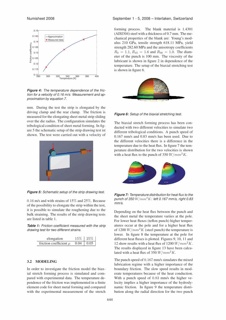
644


280 300 320 340 360 380 4000.11

0.115

0.12

0.125

0.13

0.135

0.14

0.145

0.15

Temperature [K]

Frict

ion

coef

ficie

nt µ

ApproximationMeasured data

Figure 4: The temperature dependence of the fric-tion for a velocity of 0.16 m/s: Measurement and ap-proximation by equation 7.

mm. During the test the strip is elongated by thedriving clamp and the rear clamp. The friction ismeasured for the elongating sheet metal strip slidingover the die radius. The configuration simulates thetribological condition of sheet metal forming. In fig-ure 5 the schematic setup of the strip drawing test istshown. The test were carried out with a velocity of

Figure 5: Schematic setup of the strip drawing test.

0.16m/s and with strains of 15% and 25%. Becauseof the possibility to elongate the strip within the test,it is possible to simulate the roughening due to thebulk straining. The results of the strip drawing testsare listed in table 1.

Table 1: Friction coefficient measured with the stripdrawing test for two different strains.

elongation 15% 25%friction coefficient µ 0.04 0.05

3.2 MODELING

In order to investigate the friction model the biax-ial stretch forming process is simulated and com-pared with experimental data. The temperature de-pendence of the friction was implemented in a finiteelement code for sheet metal forming and comparedwith the experimental measurement of the stretch

forming process. The blank material is 1.4301(AISI304) steel with a thickness of 0.7 mm. Theme-chanical properties of the blank are: Young’s mod-ulus 210 GPa, tensile strength 618.11 MPa, yieldstrength 282.60 MPa and the anisotropy coefficientsR0 = 1.1, R45 = 1.6 and R90 = 1.0. The diam-eter of the punch is 100 mm. The viscosity of thelubricant is shown in figure 2 in dependence of thetemperature. The setup of the biaxial stretching testis shown in figure 6.

Figure 6: Setup of the biaxial stretching test.

The biaxial stretch forming process has been con-ducted with two different velocities to simulate twodifferent tribological conditions. A punch speed of0.167 mm/s and 0.83 mm/s has been used. Due tothe different velocities there is a difference in thetemperature due to the heat flux. In figure 7 the tem-perature distribution for the two velocities is shownwith a heat flux to the punch of 350 W/mm2K .

Figure 7: Temperature distribution for heat flux to thepunch of 350 W/mm2K: left 0.167 mm/s, right 0.83mm/s.

Depending on the heat flux between the punch andthe sheet metal the temperature variies at the pole.For lower heat fluxes (teflon punch) higher temper-atures occur at the pole and for a higher heat fluxof 1200W/mm2K (steel punch) the temperature islower. In figure 8 the temperature at the pole fordifferent heat fluxes is plotted. Figures 9, 10, 11 and12 show results with a heat flux of 1200W/mm2K .The results displayed in figure 13 have been calcu-lated with a heat flux of 350 W/mm2K .

The punch speed of 0.167mm/s simulates the mixedlubrication regime with a higher importance of theboundary friction. The slow speed results in mod-erate temperatures because of the heat conduction.With a punch speed of 0.83 mm/s the higher ve-locity implies a higher importance of the hydrody-namic friction. In figure 9 the temperature distri-bution along the radial direction for the two punch

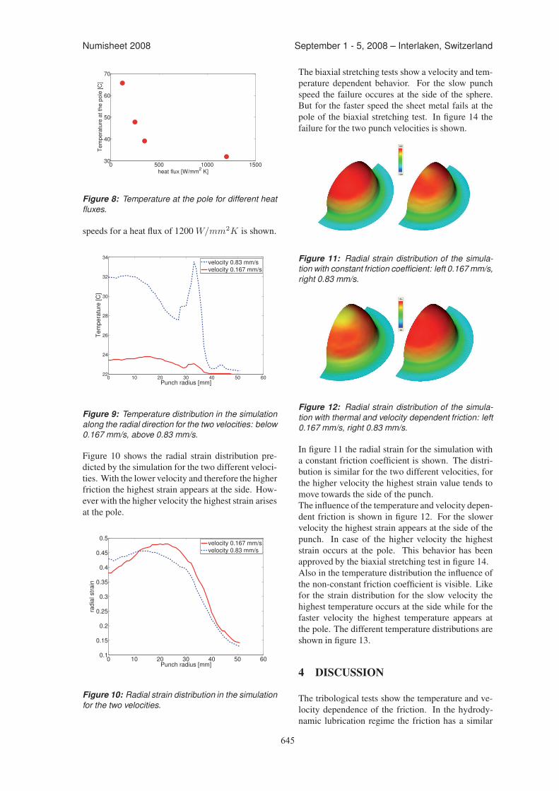
645


0 500 1000 150030

40

50

60

70

heat flux [W/mm2 K]

Tem

pera

ture

at t

he p

ole

[C]

Figure 8: Temperature at the pole for different heatfluxes.

speeds for a heat flux of 1200 W/mm2K is shown.

0 10 20 30 40 50 6022

24

26

28

30

32

34

Punch radius [mm]

Tem

pera

ture

[C]

velocity 0.83 mm/svelocity 0.167 mm/s

Figure 9: Temperature distribution in the simulationalong the radial direction for the two velocities: below0.167 mm/s, above 0.83 mm/s.

Figure 10 shows the radial strain distribution pre-dicted by the simulation for the two different veloci-ties. With the lower velocity and therefore the higherfriction the highest strain appears at the side. How-ever with the higher velocity the highest strain arisesat the pole.

0 10 20 30 40 50 600.1

0.15

0.2

0.25

0.3

0.35

0.4

0.45

0.5

Punch radius [mm]

radi

al s

train

velocity 0.167 mm/svelocity 0.83 mm/s

Figure 10: Radial strain distribution in the simulationfor the two velocities.

The biaxial stretching tests show a velocity and tem-perature dependent behavior. For the slow punchspeed the failure occures at the side of the sphere.But for the faster speed the sheet metal fails at thepole of the biaxial stretching test. In figure 14 thefailure for the two punch velocities is shown.

Figure 11: Radial strain distribution of the simula-tion with constant friction coefficient: left 0.167mm/s,right 0.83 mm/s.

Figure 12: Radial strain distribution of the simula-tion with thermal and velocity dependent friction: left0.167 mm/s, right 0.83 mm/s.

In figure 11 the radial strain for the simulation witha constant friction coefficient is shown. The distri-bution is similar for the two different velocities, forthe higher velocity the highest strain value tends tomove towards the side of the punch.The influence of the temperature and velocity depen-dent friction is shown in figure 12. For the slowervelocity the highest strain appears at the side of thepunch. In case of the higher velocity the higheststrain occurs at the pole. This behavior has beenapproved by the biaxial stretching test in figure 14.Also in the temperature distribution the influence ofthe non-constant friction coefficient is visible. Likefor the strain distribution for the slow velocity thehighest temperature occurs at the side while for thefaster velocity the highest temperature appears atthe pole. The different temperature distributions areshown in figure 13.

4 DISCUSSION

The tribological tests show the temperature and ve-locity dependence of the friction. In the hydrody-namic lubrication regime the friction has a similar

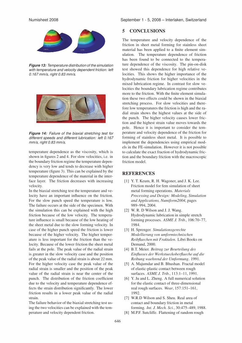
646


Figure 13: Temperature distribution of the simulationwith temperature and velocity dependent friction: left0.167 mm/s, right 0.83 mm/s.

Figure 14: Failure of the biaxial stretching test fordifferent speeds and different lubrication: left 0.167mm/s, right 0.83 mm/s.

temperature dependence as the viscosity, which isshown in figures 2 and 4. For slow velocities, i.e. inthe boundary friction regime the temperature depen-dency is very low and tends to decrease with highertemperature (figure 3). This can be explained by thetemperature dependence of the material in the inter-face layer. The friction decreases with increasingvelocity.In the biaxial stretching test the temperature and ve-locity have an important influence on the friction.For the slow punch speed the temperature is low.The failure occurs at the side of the specimen. Withthe simulation this can be explained with the highfriction because of the low velocity. The tempera-ture influence is small because of the low heating ofthe sheet metal due to the slow forming velocity. Incase of the higher punch speed the friction is lowerbecause of the higher velocity. The higher temper-ature is less important for the friction than the ve-locity. Because of the lower friction the sheet metalfails at the pole. The peak value of the radial strainis greater in the slow velocity case and the positionof the peak value of the radial strain is about 22mm.For the higher velocity case the peak value of theradial strain is smaller and the position of the peakvalue of the radial strain is near the center of thepunch. The distribution of the friction coefficientdue to the velocity and temperature dependence ef-fects the strain distribution significantly. The lowerfriction results in a lower peak value of the radialstrain.The failure behavior of the biaxial stretching test us-ing the two velocities can be explained with the tem-perature and velocity dependent friction.

5 CONCLUSIONSThe temperature and velocity dependence of thefriction in sheet metal forming for stainless sheetmaterial has been applied to a finite element sim-ulation. The temperature dependence of frictionhas been found to be connected to the tempera-ture dependence of the viscosity. The pin-on-disktest showed this dependence for high relative ve-locities. This shows the higher importance of thehydrodynamic friction for higher velocities in themixed lubrication regime. In contrast for slow ve-locities the boundary lubrication regime contributesmore to the friction. With the finite element simula-tion these two effects could be shown in the biaxialstretching process. For slow velocities and there-fore low temperatures the friction is high and the ra-dial strain shows the highest values at the side ofthe punch. The higher velocity causes lower fric-tion and the highest strain value moves towards thepole. Hence it is important to consider the tem-perature and velocity dependence of the friction forforming of stainless sheet metal. It is possible toimplement the dependencies using empirical mod-els in the FE-simulation. However it is not possibleto calculate the exact fraction of hydrodynamic fric-tion and the boundary friction with the macroscopicfriction model.

REFERENCES[1] Y. T. Keum, R. H. Wagoner, and J. K. Lee.

Friction model for fem simulation of sheetmetal forming operations. MaterialsProcessing and Design: Modeling, Simulationand Applications, Numiform2004, pages989–994, 2004.

[2] W. R. D Wilson and J. J. Wang.Hydrodynamic lubrication in simple stretchforming processes. ASME J. Trib., 106:70–77,1984.

[3] H. Sprenger. SimulationsgerechteModellierung von umformtechnischenReibflaechen mit Fraktalen. Libri Books onDemand, 2000.

[4] B.T. Meier. Beitrag zur Beurteilung desEinflusses der Werkstueckoberflaeche auf dieReibung waehrend der Umformung. 1991.

[5] A. Majumdar and B. Bhushan. Fractal modelof elastic-plastic contact between roughsurfaces. ASME J. Trib., 113:1–11, 1991.

[6] Y. Ju and L. Zheng. A full numerical solutionfor the elastic contact of three-dimensionalreal rough surfaces. Wear, 157:151–161,1992.

[7] W.R.D Wilson and S. Sheu. Real area ofcontact and boundary friction in metalforming. Int. J. Mech. Sci., 30:475–489, 1988.

[8] M.P.F. Sutcliffe. Flattening of random rough

647


surfaces in metal forming processes. ASME J.Trib., 121:433–440, 1999.

[9] S. W. Lo and T. S. Yang. A new mechanismof asperity flattening in sliding contact - therole of elastic tool microwedge. ASME J.Trib., 125:713–719, 2003.

[10] R. Grueebler and P. Hora. Modeling ofsurface texturing of sheet metal and tool insheet metal processes. Proceeding ofICTMP07, 2007.

[11] F. P. Bowden and D. Tabor. The Friction andLubrication of Solids. Clarendon Press, 1986.

[12] H. Vogel. DasTemperaturabhaengigkeitsgesetz derViskositaet von Fluessigkeiten. PhysikalischeZeitschrift, XXII:645–646, 1921.

Documents

08 Numisheet2008 Hot Forming Chapter8