08-fs

8/3/2019 08-fs

http://slidepdf.com/reader/full/08-fs 1/13

Fourier Series

Much of this course concerns the problem of representing a function as a sum of its different frequency

components. Expressing a musical tone as a sum of a fundamental tone and various harmonics is such a

representation. So is a spectral decomposition of light waves. The ability to isolate the signal of a single

radio or television station from the dozens that are being simultaneously received depends on being able to

amplify certain frequencies and suppress others.

We start our look at the theory of Fourier series with two questions:

Question #1

Which functions f (t) have a representation as a sum of constants times cos( kt)’s and sin(kt)’s? Since cos(kt)

and sin(kt) can be written in terms of complex exponentials(1) using

cos(kt) = 12

eikt + e−ikt

sin(kt) = 1

2i

eikt − e−ikt

and, conversely, e±ikt

can be written in terms of cos(kt)’s and sin(kt)’s usinge±ikt = cos(kt) ± i sin(±kt)

it is equivalent to ask which functions f (t) have a representation

f (t) =∞

k=−∞ckeikt (1)

for some constants ck. Because it will save us considerable writing we shall start with this form of the

question and return to sines and cosines later.

First, observe that, for every integer k, eikt = cos(kt) + i sin(kt) is periodic with period 2π. So the right

hand side is necessarily periodic of period 2π. Unless f (t) is periodic with period 2π, it cannot possibly have

a representation of the form (1). We shall shortly state a result that says that, on the other hand, everysufficiently continuous (details later) function of period 2π has a representation (1). In this course, we shall

never fully justify this claim. On the other hand, it is fairly easy justify an analogous claim for “Discrete

Fourier Series”, which is the version of Fourier series for functions f (t) that are only defined for t = nτ , with

n running over the integers and τ a fixed spacing. This is done in the notes “Discrete–Time Fourier Series

and Fourier Transforms”. Before giving the detailed answer to this question, we consider

Question #2

Suppose that we know that some specific function f (t) has a representation of the form (1). What are the

values of the coefficients ck? With a little trickery, we shall be able to answer this question completely and

easily. We wish to solve (1) for the ck’s. At first this task looks somewhat daunting because (1) is really a

system of infinitely many equations (one equation for each value of t) in infinitely many unknowns (the ck’s).The trick will allow us to reduce this system to a single equation in any one unknown. Suppose, for example,

that we wish to solve for c17. The index 17 has been chosen at random. Then we use the “orthogonality

relation” that, when k = 17, π−π

eikte−i17t dt =

π−π

ei(k−17)t dt = 1i(k−17)

ei(k−17)tπ−π = 1

i(k−17)

ei(k−17)π − e−i(k−17)π

= 0 (2)

(1) See the notes entitled “Complex Numbers and Exponentials”

February 4, 2007 Fourier Series 1

8/3/2019 08-fs


(because ei(k−17)π/e−i(k−17)π = ei(k−17)2π = 1 so that ei(k−17)π = e−i(k−17)π for all integers k) to eliminate

all the ck’s with k = 17 from (1). To do so, take (1), multiply it by e−i17t and integrate the result from −π

to π. This gives π−π

f (t)e−i17t dt =

∞k=−∞

ck

π−π

eikte−i17t dt

Because of (2), all of the terms on the right hand side with k = 17 are zero. Thus π−π

f (t)e−i17t dt = c17

π−π

ei17te−i17t dt = c17

π−π

dt = 2π c17

As promised, this is a single equation in the single unknown c17, which we can trivially solve.

c17 = 12π

π−π

f (t)e−i17t dt

Of course, we could have done the same thing with the integer 17 replaced by any other integer m. This

would have given

cm = 12π π−π f (t)e−imt dt (3)

We now know all of the Fourier coefficients and are ready to return to the answer to question #1.

The Main Fourier Series Expansion.

We shall shortly construct a number of different Fourier series expansions that are used for various

different classes of functions. For all of these expansions, we are going to restrict our attention to functions

that are piecewise continuous with piecewise continuous first derivative. In applications, most functions

satisfy these regularity requirements. We start with the definition of “piecewise continuous”.

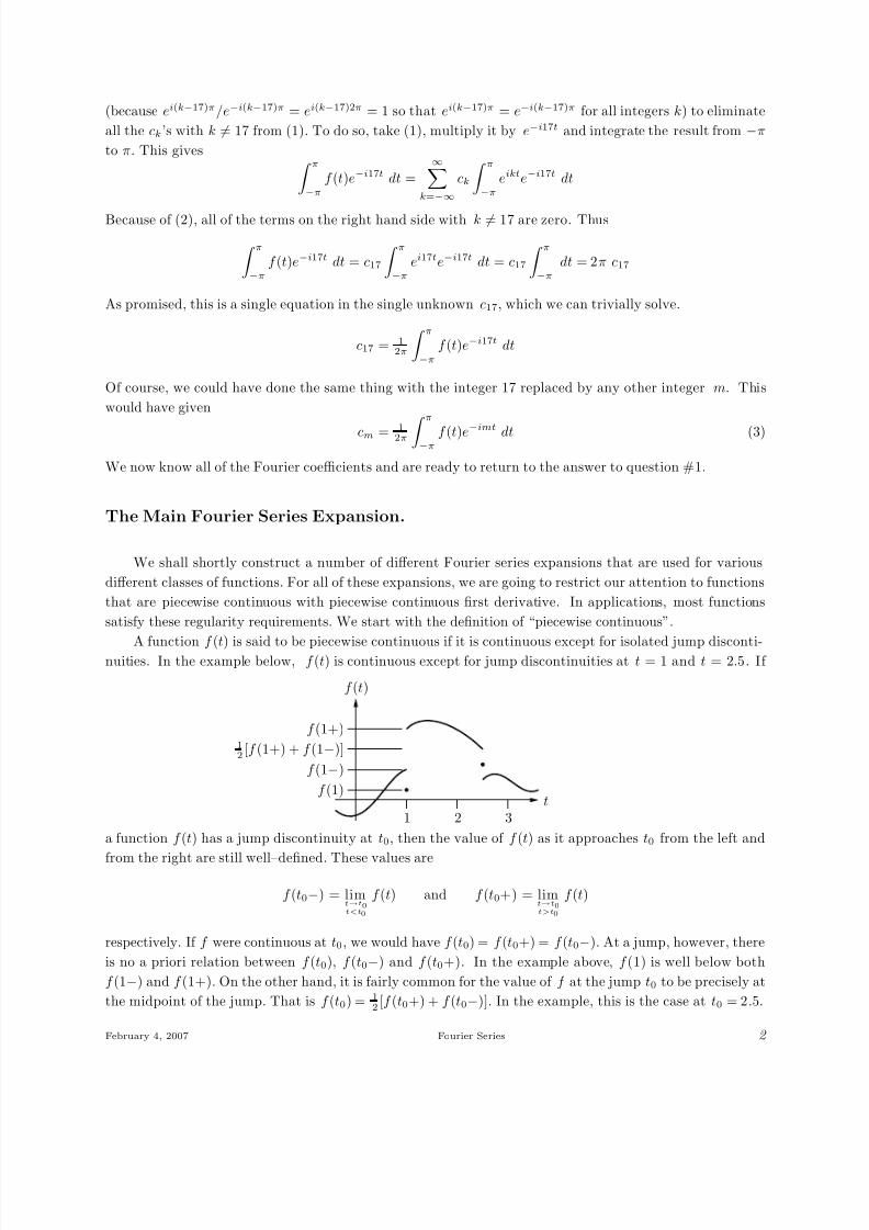
A function f (t) is said to be piecewise continuous if it is continuous except for isolated jump disconti-nuities. In the example below, f (t) is continuous except for jump discontinuities at t = 1 and t = 2.5. If

t

f (t)

1 2 3

f (1+)

f (1−)

12 [f (1+) + f (1−)]

f (1)

a function f (t) has a jump discontinuity at t0, then the value of f (t) as it approaches t0 from the left and

from the right are still well–defined. These values are

f (t0−) = limt→t0t<t0

f (t) and f (t0+) = limt→t0t>t0

f (t)

respectively. If f were continuous at t0, we would have f (t0) = f (t0+) = f (t0−). At a jump, however, there

is no a priori relation between f (t0), f (t0−) and f (t0+). In the example above, f (1) is well below both

f (1−) and f (1+). On the other hand, it is fairly common for the value of f at the jump t0 to be precisely at

the midpoint of the jump. That is f (t0) = 12 [f (t0+) + f (t0−)]. In the example, this is the case at t0 = 2.5.


8/3/2019 08-fs


8/3/2019 08-fs


This is of the form∞

k=−∞ ckeikt with

ck =

12√

2(1 − i) if k = 1

12√

2(1 + i) if k = −1

0 if k

=

−1, 1

The Fourier coefficients of a periodic function are unique. We showed this in the course of answering Question

# 2. So the right hand side of (5) is THE Fourier expansion for f (t) = sin

t + π4

. There is no need to

evaluate the integrals in (4). Not only would that be a lot of wasted effort, but we would probably make a

mechanical error along the way and end up with the wrong answer.

Example 4 Suppose that the function

f (t) =

∞k=−∞

ckeikt (6)

is real–valued for all −∞ < t < ∞. What conclusions can be drawn concerning the Fourier coefficients ck? Anumber is real if and only if it is the same as its complex conjugate. So f (t) is real if and only if f (t) = f (t).

Substituting in (6) gives that f (t) is real if and only if

∞k=−∞

ckeikt =∞

k=−∞cke−ikt =

∞k=−∞

c−keikt

For the second equality, we replaced k by −k in the sum. This is legitimate because, as k runs over all of the

integers from −∞ to +∞, −k also runs exactly once over all integers. Again by the uniqueness of Fourier

coefficients (the “only if” part of Theorem 1), the two sums are equal for all t if and only if ck = c−k for all

k. So we conclude that

f (t) is real for all −∞ < t < ∞ ⇐⇒ ck = c−k for all − ∞ < k < ∞

For example

sin t = 12i

eit − e−it

=

∞k=−∞

ckeikt with ck =

12i if k = 1− 1

2i if k = −10 otherwise

is a real–valued function and c1 and c−1 are indeed complex conjugates of each other.

Example 5 The function

f (t) =

∞

k=−∞

ckeikt (7)

is necessarily periodic of period 2π. Suppose that it is also periodic of period π. For example, the function

cos(2t) is periodic of period 2π and also periodic of period π. What conclusions can be drawn concerning the

Fourier coefficients ck? The function f (t) has period π if and only if f (t) = f (t + π) for all t. Substituting

in (7) gives that f (t) has period π if and only if

∞k=−∞

ckeikt =

∞k=−∞

ckeik(t+π) =

∞k=−∞

ckeikπ

eikt


8/3/2019 08-fs


Once again by the uniqueness of Fourier coefficients, the two sums are equal for all t if and only if ck = ckeikπ

for all k. For k even, eikπ = 1 and ck = ckeikπ is trivially true. But for k odd, eikπ = −1 and ck = ckeikπ is

true if and only if ck = 0. So we conclude that

f (t) has period π ⇐⇒ ck = 0 for all odd k

For example

cos(2t) = 12

ei2t + e−2it

=

∞k=−∞

ckeikt with ck =

12 if k = ±20 otherwise

does indeed have ck = 0 for all odd k.

Using Theorem 1, we can easily come up with lots of variations. In these variations, we shall assume

that all functions are piecewise continuous with piecewise continuous first derivative and we shall also assume

that f (t) = f (t+)+f (t−)2 for all t.

Variation #1 – period 2ℓ

It is easy to modify our Fourier series result to apply to functions that have period 2 ℓ, for some ℓ > 0,

rather than 2π. Just rename the variable t in the Fourier Series Theorem to τ and then make the change of

variables τ = πℓ

t. This gives

f (t) =∞

k=−∞ckeik

πℓt with ck = 1

2ℓ

ℓ−ℓ

f (t)e−ikπℓt dt (8)

As a check, note that since eikπℓ

(t+2ℓ) = eikπℓtei2kπ = eik

πℓt, so that eik

πℓt has period 2ℓ. The formula for ck

in (8) can be derived directly, using

ℓ−ℓ eikπℓte−im

πℓt dt = 2ℓ if k = m

0 if k = m

and the same strategy as led to (3).

Variation #2 – sin’s and cos’s

To convert (8) into sin’s and cos’s just sub in eikπℓt = cos(kπt

ℓ) + i sin(kπt

ℓ).

f (t) =

∞k=−∞

ckeikπℓt =

∞k=−∞

ck

cos(kπtℓ

) + i sin(kπtℓ

)

The k = 0 term in this sum is

c0

cos(0πtℓ ) + i sin(

0πtℓ )

= c0

The k = 1 and k = −1 terms together are

c1

cos(πt

ℓ) + i sin(πt

ℓ)

+ c−1

cos(−πt

ℓ) + i sin(−πt

ℓ)

= [c1 + c−1]cos(πtℓ

) + [ic1 − ic−1]sin(πtℓ

)

since cos(−πtℓ

) = cos(πtℓ

) and sin(−πtℓ

) = − sin(πtℓ

). Similarly, the k = 2 and k = −2 terms together are

c2

cos( 2πt

ℓ) + i sin( 2πt

ℓ)

+ c−2

cos(− 2πt

ℓ) + i sin(− 2πt

ℓ)

= [c2 + c−2] cos(2πtℓ

) + [ic2 − ic−2]sin( 2πtℓ

)


8/3/2019 08-fs


8/3/2019 08-fs


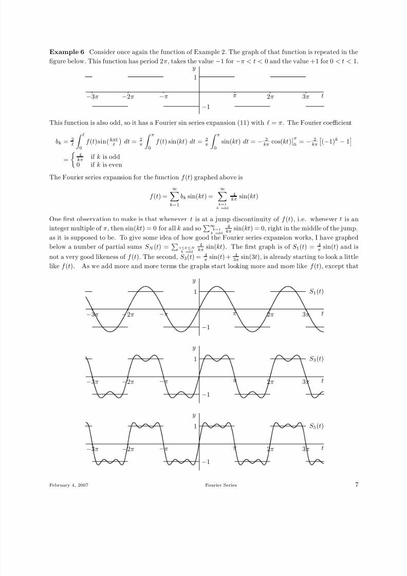
Example 6 Consider once again the function of Example 2. The graph of that function is repeated in the

figure below. This function has period 2π, takes the value −1 for −π < t < 0 and the value +1 for 0 < t < 1.y

t−

3π−

2π−

π π 2π 3π

1

−1

This function is also odd, so it has a Fourier sin series expansion (11) with ℓ = π. The Fourier coefficient

bk = 2ℓ

ℓ0

f (t)sin(kπtℓ

dt = 2

π

π0

f (t) sin(kt) dt = 2π

π0

sin(kt) dt = − 2kπ

cos(kt)π

0= − 2

kπ

(−1)k − 1

=

4kπ

if k is odd0 if k is even

The Fourier series expansion for the function f (t) graphed above is

f (t) =∞

k=1

bk sin(kt) =∞

k=1k odd

4kπ

sin(kt)

One first observation to make is that whenever t is at a jump discontinuity of f (t), i.e. whenever t is an

integer multiple of π, then sin(kt) = 0 for all k and so∞

k=1k odd

4kπ

sin(kt) = 0, right in the middle of the jump,

as it is supposed to be. To give some idea of how good the Fourier series expansion works, I have graphed

below a number of partial sums S N (t) =

1≤k≤Nk odd

4kπ

sin(kt). The first graph is of S 1(t) = 4π

sin(t) and is

not a very good likeness of f (t). The second, S 3(t) = 4π

sin(t) + 43π sin(3t), is already starting to look a little

like f (t). As we add more and more terms the graphs start looking more and more like f (t), except that

y

t−3π −2π −π π 2π 3π

1

−1

S 1(t)

y

t−3π −2π −π π 2π 3π

1

−1

S 3(t)

y

t−3π −2π −π π 2π 3π

1

−1

S 5(t)


8/3/2019 08-fs


y

t−3π −2π −π π 2π 3π

1

−1

S 19(t)

y

t−3π −2π −π π 2π 3π

1

−1

S 59(t)

they exhibit a little “ringing” right at the discontinuities. This “ringing” is always present in partial sums

of Fourier series at jump discontinuities. It is called the Gibbs phenomenon.

Example 7 As another example, we replace the jump discontinuity of the first example by a ramp. We

shall see that, even if the ramp is moderately steep, the ringing of Gibbs phenomenon disappears. Just to

put in an additional change, I’ll make the function even rather than odd. Its graph is given in the figure

below. This function has period 2π, takes the value 1 for 0 < t < a and decreases from 1 down to 0 and t

runs from a up to π. For 0 ≤ t ≤ π, the function is given by the formula

f (t) =

1 if 0 ≤ t ≤ aπ−tπ−a if a ≤ t ≤ π

This function is also even, so it has a Fourier cosine series expansion (12) with ℓ = π. The Fourier coefficient,y

t−3π −2π −π πa 2π 3π

1

for k = 0, is

ak = 2ℓ

ℓ0

f (t) cos(kπtℓ

dt = 2

π

π0

f (t) cos(kt) dt = 2π

a0

cos(kt) dt + 2π

πa

π−tπ−a cos(kt) dt

To evaluate these integrals we need the indefinite integrals of cos( kt) and t cos(kt). The first one is trivial

cos(kt) dt = 1

k sin(kt) + C

The second is normally computed using integration by parts. But it is easier to just apply ddk

to both sides

of sin(kt) dt = − 1

k cos(kt) + C

Note that, while we only need this integral for integer k, it is valid for all nonzero k. So it is legitimate to

differentiate with respect to k. Also note that, while the “constant” C is independent of t, it is allowed to


8/3/2019 08-fs


depend on k, so its derivative with respect to k need not be zero. In any event, applying ddk

gives t cos(kt) dt = t

ksin(kt) + 1

k2cos(kt) + C ′

so thatak = 2

kπsin(kt)

a

0+ 2

k(π−a) sin(kt)

π

a− 2

π(π−a)

tk

sin(kt) + 1k2

cos(kt)

π

a

= 2kπ −

2k(π−a)

sin(ka) −

2(−

1)k

k2π(π−a) +2

π(π−a)ak sin(ka) +

1k2 cos(ka)

For k = 0,

a0 = 2ℓ

ℓ0

f (t)cos( 0πtℓ

dt = 2

π

π0

f (t) dt

The integral is the area under the graph for 0 ≤ t ≤ π. The region under the graph consists of a rectangle

of height 1 and base a and a triangle of height 1 and base π − a. So

a0 = 2π

a + 1

2 (π − a)

= 1 + aπ

The Fourier series expansion for the function f (t) graphed above is

f (t) = a02 +

∞k=1

ak cos(kt)

with the ak’s given above. these ak’s are a little messy to compute by hand, but easy to program. Onceagain, I have had my computer graph a number of partial sums S N (t) = a0

2 +N −1

k=1 ak cos(kt), for a specific

choice of the ramp parameter a, namely a = 0.9π. The first graph is of S 1(t) = 1 + aπ

is just a straight line

whose height is the average value of f (t). This time we get a really good likeness of the graph of f (t) before

we have included a hundred terms.

y


1

S 1(t)

y


1

S 4(t)

y


1

S 8(t)

y


1

S 16(t)


8/3/2019 08-fs


y


1S 32(t)

y


1S 64(t)

Example 8 By a standard trig identity, the periodic function f (t) = cos2 t obeys

f (t) = cos2 t = 12 + 1

2 cos(2t) (13)

The right hand side is a Fourier cosine expansion a02 +

∞k=1 ak cos(kt) with a0 = 1, a2 = 1

2 and all other ak’s

zero. Just as in the complex case, the coefficients in the real Fourier expansions are uniquely determined.

So the right hand side of (13) is the Fourier expansion for f (t) = cos2 t.

Application of Fourier Series to Ordinary Differential Equations.

Consider the RLC circuit

+

−x(t)

R L

C i(t)

+

−

y(t)

We’re going to think of the voltage x(t) as a input signal and the voltage y(t) as an output signal. The goal

is to determine the output voltage for any given input voltage. If i(t) is the current flowing at time t in the

loop as shown and q(t) is the charge on the capacitor, then the voltage across R, L and C , respectively, at

time t are Ri(t), L didt

(t) and y(t) =q(t)C

. By Kirchhoff’s law, these three voltages must add up to x(t) so that

Ri(t) + L di

dt

(t) + q(t)

C

= x(t) (14)

This is one equation in the two unknowns, i(t) and q(t). Fortunately, there is a relationship between the

two. Namely

i(t) = dqdt

(t) = Cy ′(t) (15)

This just says that the capacitor cannot create or destroy charge on its own. All charging of the capacitor

must come from the current. Subbing (15) into (14) gives

LCy ′′(t) + RCy ′(t) + y(t) = x(t) (16)


8/3/2019 08-fs


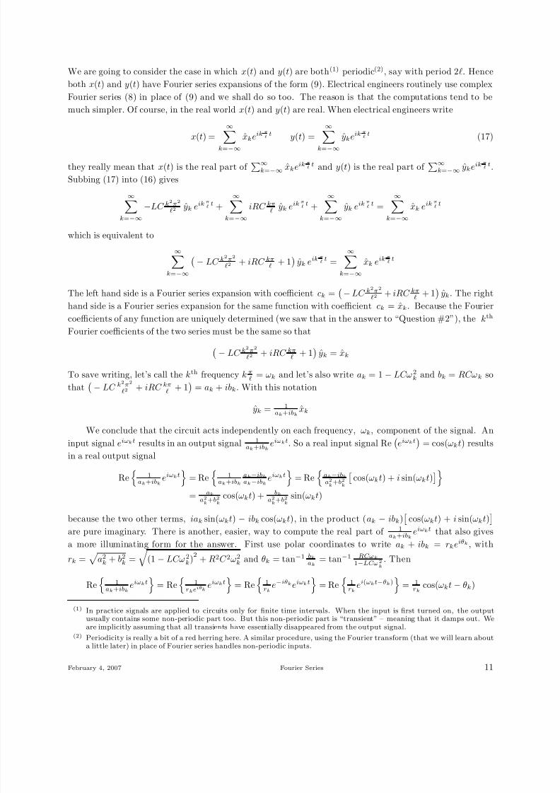
We are going to consider the case in which x(t) and y(t) are both(1) periodic(2), say with period 2ℓ. Hence

both x(t) and y(t) have Fourier series expansions of the form (9). Electrical engineers routinely use complex

Fourier series (8) in place of (9) and we shall do so too. The reason is that the computations tend to be

much simpler. Of course, in the real world x(t) and y(t) are real. When electrical engineers write

x(t) =

∞k=−∞ xke

ik πℓt

y(t) =

∞k=−∞ yke

ik πℓt

(17)

they really mean that x(t) is the real part of ∞

k=−∞ xkeikπℓt and y(t) is the real part of

∞k=−∞ ykeik

πℓt.

Subbing (17) into (16) gives

∞k=−∞

−LC k2π2

ℓ2yk eik

πℓt +

∞k=−∞

iRC kπℓ

yk eikπℓt +

∞k=−∞

yk eikπℓt =

∞k=−∞

xk eikπℓt

which is equivalent to

∞

k=−∞

− LC k2π2

ℓ2+ iRC kπ

ℓ+ 1

yk eikπℓt =

∞

k=−∞

xk eikπℓt

The left hand side is a Fourier series expansion with coefficient ck =− LC k

2π2

ℓ2+ iRC kπ

ℓ+ 1

yk. The right

hand side is a Fourier series expansion for the same function with coefficient ck = xk. Because the Fourier

coefficients of any function are uniquely determined (we saw that in the answer to “Question #2”), the kth

Fourier coefficients of the two series must be the same so that

− LC k2π2

ℓ2+ iRC kπ

ℓ+ 1

yk = xk

To save writing, let’s call the kth frequency k πℓ

= ωk and let’s also write ak = 1 − LCω 2k and bk = RCωk so

that− LC k

2π2

ℓ2+ iRC kπ

ℓ+ 1

= ak + ibk. With this notation

yk = 1ak+ibk

xk

We conclude that the circuit acts independently on each frequency, ωk, component of the signal. An

input signal eiωkt results in an output signal 1ak+ibk

eiωkt. So a real input signal Re

eiωkt

= cos(ωkt) results

in a real output signal

Re

1ak+ibk

eiωkt

= Re

1ak+ibk

ak−ibkak−ibk eiωkt

= Re

ak−ibka2k

+b2k

cos(ωkt) + i sin(ωkt)

= ak

a2k

+b2k

cos(ωkt) + bka2k

+b2k

sin(ωkt)

because the two other terms, iak sin(ωkt) − ibk cos(ωkt), in the product (ak − ibk)

cos(ωkt) + i sin(ωkt)

are pure imaginary. There is another, easier, way to compute the real part of 1ak+ibk

eiωkt that also gives

a more illuminating form for the answer. First use polar coordinates to write ak + ibk = rkeiθk , with

rk =

a2k + b2

k =

(1 − LCω 2k)2 + R2C 2ω2

k and θk = tan−1 bkak

= tan−1 RCωk1−LCω2

k. Then

Re

1ak+ibk

eiωkt

= Re

1rke

iθkeiωkt

= Re

1rk

e−iθkeiωkt

= Re

1rk

ei(ωkt−θk)

= 1rk

cos(ωkt − θk)

(1) In practice signals are applied to circuits only for finite time intervals. When the input is first turned on, the outputusually contains some non-periodic part too. But this non-periodic part is “transient” – meaning that it damps out. Weare implicitly assuming that all transients have essentially disappeared from the output signal.

(2) Periodicity is really a bit of a red herring here. A similar procedure, using the Fourier transform (that we will learn abouta little later) in place of Fourier series handles non-periodic inputs.


8/3/2019 08-fs


So the RLC cricuit has two effects on the frequency ωk part of the input signal. Its amplitude is

multiplied by 1rk

= 1√(1−LCω2

k)2+R2C 2ω2

k

and it also undergoes a phase shift θk = tan−1 RCωk1−LCω2

k

. Here is a

graph of A = 1√(1−LCω2)2+R2C 2ω2

against ω

ω

A

Note that there is a small range of frequencies that give a large amplitude response. This is the phenomenon

of resonance. That is why this circuit is often used as a filter to extract a specific frequency from the input

signal.

Power and Parseval’s Relation

The energy carried by a signal f (t) is ∞−∞ |f (t)|2 dt. For a (nonzero) periodic signal this is always

infinite. So for a periodic signal the average power (energy per unit time) is a much more useful quantity. If

f (t) has period 2ℓ, it has average power

P = 12ℓ

ℓ−ℓ

|f (t)|2 dt

We can express this power in terms of the Fourier coefficients of f just by substituting f (t) =∞

k=−∞ ckeikπℓt

P = 12ℓ

ℓ

−ℓ

f (t)f (t) dt = 12ℓ

∞

k,m=−∞

ℓ

−ℓ

ckeikπℓtcmeim

πℓt dt = 1

2ℓ

∞

k,m=−∞

ckcm ℓ

−ℓ

ei(k−m) πℓt dt

By the orthogonality relation (2), with 17 replaced by m,

ℓ−ℓ

ei(k−m)πℓt dt =

2ℓ if k = m0 otherwise

So all of the terms in the double sum with k = m are zero and we are left with

P = 12ℓ

ℓ−ℓ

|f (t)|2 dt = 12ℓ

∞k,m=−∞k=m

ckcm 2ℓ =∞

k=−∞|ck|2 (18)

This is called Parseval’s relation. To convert it into a statement about the Fourier coefficients ak, bk, we

just need observe, from (10), that c0 = 12

a0 and, for k > 0, ck = 12 (ak − ibk), c−k = 1

2 (ak + ibk). Assuming

that ak and bk are real, |c0|2 = 14 |a0|2 and, for k > 0, |ck|2 = |c−k|2 = 1

4 [a2k + b2

k] so that

P = 12ℓ

ℓ−ℓ

|f (t)|2 dt = 14 a2

0 + 12

∞k=1

a2k + b2

k

Suppose that we have some complicated signal f (t) =∞

k=−∞ ckeikπℓt and we wish to approximate it by

a simple signal that only contains the finite number of frequencies k πℓ

with, for example, k = −2, −1, 0, 1, 2.


8/3/2019 08-fs


That is, our approximating signal is to be of the form F (t) = d−2e−2iπℓt + d−1e−i

πℓt + d0 + d1ei

πℓt + d2e2iπ

ℓt.

What should we choose for the coefficients d−2, d−1, d0, d1 and d2? To ensure the the error carries minimum

average power, we should choose the coefficients so that

12ℓ

ℓ

−ℓ

|f (t) − F (t)|2 dt

is as small as possible. Since

f (t) − F (t) =

∞k=−∞

ckeikπℓt

− 2k=−2

dkeikπℓt

=

∞k=−∞

ekeikπℓt

with

ek =

ck − dk if |k| ≤ 2ck otherwise

Parseval’s relation (18) gives that the average power carried by the error is

12ℓ ℓ−ℓ |f (t) − F (t)|2 dt =

∞k=−∞

|ek|2 =

∞−2≤k≤2

|ck − dk|2 +

∞−∞<k<∞|k|>2

|ck|2

This is minimised by choosing dk = ck for all −2 ≤ k ≤ 2.

Example 9 By Example 2, the function

f (t) =

1 if 0 < t < π−1 if −π < t < 0

f (t) = f (t + 2π)

has Fourier coefficients

ck = − 2

kπi if k is odd

0 if k is even

So Parseval’s relation (18) gives that

12π

π−π

|f (t)|2 dt =

−∞<k<∞k odd

− i 2kπ

2 =

−∞<k<∞k odd

4k2π2

=

0<k<∞k odd

8k2π2

Since 12π

π−π |f (t)|2 dt = 1

2π

π−π 1 dt = 1, we conclude that

0<k<∞k odd

8k2π2

= 1 or 112 + 1

32 + 152 + · · · = π2

8


Documents

08-fs