3D GPR surveys on Friesland dike

2007

Tomi Herronen & Timo Saarenketo

1. Introduction In May 2007 Roadscanners did a series of Ground Penetrating Radar (GPR) surveys on two dikes in the Netherlands, one in Friesland and the other in Hellegatsdam. The purpose of these surveys was to determine pavement layer thickness for safety assessment reasons and to produce seed thickness values for FWD back calculation. Another goal was to locate degradation, cracks, voids and other indicators of poor quality structure in the top layers of the dikes. For this task a 3d ground penetrating radar technique was chosen to provide better area coverage over the dike. With a traditional single channel GPR system the limiting factor is that it only gives information along a single narrow line. A 3d GPR collects data from a 2.4 m wide area in a single run, providing a three dimensional view of the dike structures. The surveys were ordered by KOAC-NPC, contact person Arjan De Looff. This report provides a summary of the key research results from the Friesland (Koehool-Westhoek) dike.

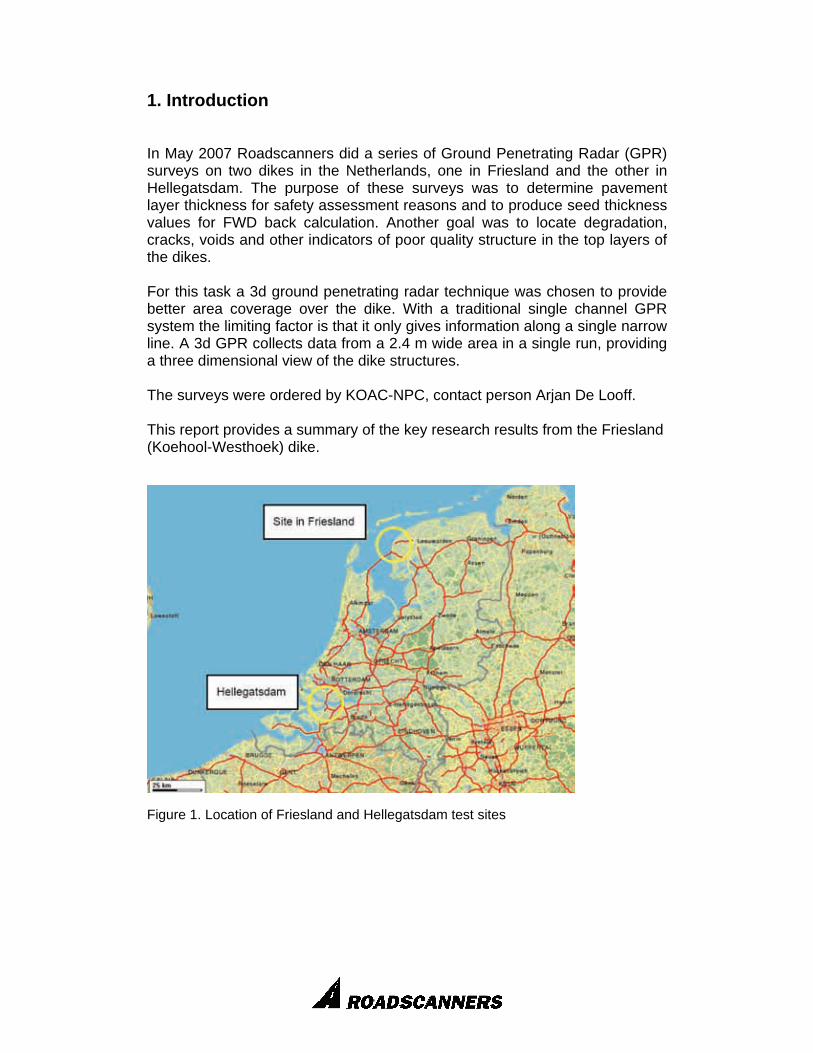
Figure 1. Location of Friesland and Hellegatsdam test sites

2. 3d Ground Penetrating Radar (GPR) Technique There are several multichannel GPR systems on the market that can be called 3d GPR. In most of the 3d GPR feasibility surveys conducted during the last few years, Roadscanners Oy has been using a Geoscope 3d-radar system which was developed and manufactured by the Norwegian firm, 3d-radar As (see Fig. 2). To analyse the data, Roadscanners has developed a special 3d Module for its Road Doctor software. During 3d Radar data collection the transmitter antenna sends a pulse into the road and the reflections from the layer interfaces are received by a receiver antenna and its’ amplitude and frequency are measured. This process is repeated rapidly through a frequency range of 100 MHz to 2000 MHz at 2 MHz steps and through all the channels (antennas) (see Fig. 3). The resulting frequency domain data will later be processed into time-domain format and interpreted as a conventional pulse radar profile.

Fig 2. Geoscope 3d –GPR with 2.4 m wide and 31 channel antenna array mounted on a survey vehicle. During data collection the Geoscope’s wheel mounted encoder controls the interval at which scans are recorded. The resulting files have a maximum of 31 parallel longitudinal profiles that present the possibility to easily compare differences (anomalies) in the structure layers.

Fig 3. Schematic picture of a 3d antenna array. The antenna consists of several transmitter-receiver antenna pairings.

3. Surveys conducted

In this work a specific section, marked on the site, of the Friesland dike was surveyed. The width of this special test section was approximately 17 m and 50 m in length. Data collection was done utilising 31 channels and using the full width of the antenna. The channel separation was 7,5 cm and the sampling interval was 10 cm, as a result of these settings the data is collected in a 7,5 * 7,5 cm grid. Survey speed was about 3 km/h. Additionally the same section was surveyed with a traditional single channel GPR, specifically a GSSI 1.0 GHz horn antenna. A total of 16 lines were measured with a separation of 1 m. Digital video was also collected in several runs over the section in order to visually inspect pavement surface damage. The collected data was then processed and interpreted with Road Doctor-software using the 3d module. With this module GPR data can be viewed as longitudinal lines, cross sections and as time slices from different depths. In the depth and time slice calculations a dielectric value of 7 was used. Figure 4 presents a view of the Road Doctor user interface while working with the Friesland data. Processing included filtering and gaining operations. The horn antenna data was preprocessed for height correction and to produce dielectric value data. Different filters and gaining settings were used in time slice view production to enhance anomalies of different type; frequency, depth or amplitude. The time slices are presented in the form that 0 m is on lower part of the dike and 16 m the upper part/top of the dike.

Fig 4. An example of 3d Radar data from the Friesland test site presented with Road Doctor software. Data shows GPR longitudinal section and cross section on the top and a time slice calculated from a depth of 10 cm. Bright colors indicate high reflection amplitude and high moisture content. 4. Results 4.1 General Friesland dike asphalt thickness results have been delivered to the customer, according to their specifications, in the form of Excel files. The results of this survey were sent to the customers in digital format. When comparing the two different GPR methods, it seems that the 3d radar provides an easier way to collect and analyse wide areas efficiently. It also gives better depth penetration than the horn-antenna. However the horn antenna is better for inspecting the upper part of the surface layer because of its’ higher resolution and more reliable amplitude and dielectric value calculations. Roadscanners Oy is continuously developing processing and analysis software to improve data handling possibilities and quality with 3d GPR.

The following text provides some special notes and findings from the survey results. 4.2 3d GPR data The collected 3d GPR data proved to be good for finding anomalies in different structure layers. In appendix 1 there are a lot of “radargrams” or time slices from various depths showing strongly or weakly reflecting areas, indicating differences in the structural integrity of a layer. The reasons for these anomalies are usually higher air, water or saline content. One problem with the Friesland with 3d GPR data was that authors could not find good processing algorithms to make the asphalt-unbound layer interface clear and, as such, the thickness interpretation was made using only the 1.0 GHz horn antenna data (see chapter 4.3). Fig 5. 3d Radar data and time slice calculated from a depth of 6 cm at the Friesland test site. One larger anomaly can bee seen from 40 to 43 m in the GPR time-slice data.

Defect?

Bottom/sea

Top

Time slice6 cm depth (Er=7)

Defect?

Bottom/sea

Top

Time slice6 cm depth (Er=7)

Fig 6. 3d Radar data and time slice calculated from a depth of 19 cm at the Friesland test site. Some interesting features are circled in the time-slice window. 4.3 GSSI 1.0 Ghz horn antenna data Unlike 3d Radar data the thickness of the asphalt was really easy to interpret from the 1.0 Ghz horn antenna data. Figure 7 provides an example of the data set and a contour map of the thickness of the profile. In the thickness calculation the surface dielectric value of the asphalt was used for the whole layer – and this might be a source of small error in the thickness calculations. These high dielectric values can be seen in the contour map of the asphalt surface dielectric values presented in figure 8. This shows that high dielectric values are located close to the sea but also in some linear sections going up the dike. These sharp linear sections with high dielectric variations can be seen even more clearly in figure 9 which presents the absolute value profiles from each section. These areas of high dielectric value and high deviation have proven to be very good indicators of distress close to the asphalt surface in many past Roadscanners projects done in Finland, Sweden, Poland, Germany and USA. Figure 10 presents a comparison of surface dielectrics and drill core verification data provided by KOAC. Even though the data does not match

perfectly it shows that solid cores were all taken from places with low dielectric values and no deviation. Fig 7. A 1.0 Ghz horn antenna GPR profile (line 0 m, closest to the sea) with asphalt thickness interpretation and a contour map presenting the thickness throughout the survey section. Red indicates thick asphalt and blue thin asphalt. In the contour map y-axis, 0 m is close to sea and 14 m on the upper side of the dike. Figure 8. A 1.0 Ghz horn antenna GPR profile (line 3 m up from the bottom of the dike) with asphalt thickness interpretation. The lower contour map presents the dielectric value of the asphalt surface where blue colours represent low dielectric values (sound asphalt) and red colors high dielectric values (asphalt adsorbs water).

Figure 9. Asphalt surface dielectric profiles measured from 15 surveys lines at the Friesland test site.

Figure 10. Comparison of surface dielectric values and drill core data taken from the Friesland dike. Black dots present separated drill cores, grey dots present partly separated and white dots present solid cores. Road Doctor software also allows calculation of some attenuation parameters from the GPR data that can be used to evaluate if the asphalt is saturated with sea water or with rain water. Figure 11 present one example of such a map, where attenuation was calculated from the asphalt at a level of 3 ns (16-18 cm) and from the unbound material at a level of 6 ns (34-36 cm).

seaside

Upper dike

seaside

Upper dike

Figure 11. A GPR data profile and attenuation map calculated from 3 ns and 6 ns. Red colors present high attenuation (salty sea water?) and blue colors lower attenuation (rain water).

Attenuation 3 ns

Attenuation 6 ns

1.0 Ghz Horn antenna data, channel 1

Attenuation 3 ns

Attenuation 6 ns

1.0 Ghz Horn antenna data, channel 1

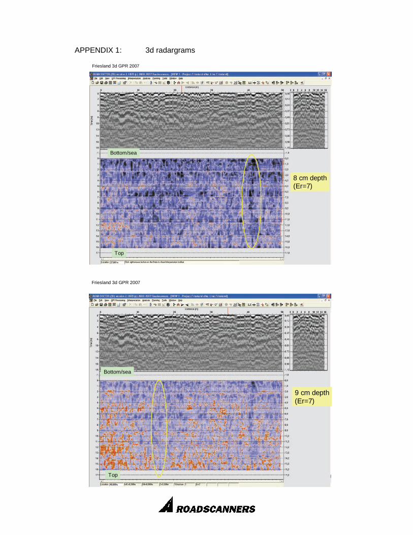
APPENDIXES APPENDIX 1: 3d radargrams

Bottom/sea

Top

9 cm depth(Er=7)

Friesland 3d GPR 2007

Bottom/sea

Top

8 cm depth(Er=7)

Friesland 3d GPR 2007

APPENDIX 1: 3d radargrams

Bottom/sea

Top

19 cm depth(Er=7)

Friesland 3d GPR 2007

Bottom/sea

Top

7 cm depth (Er=7)

Friesland 3d GPR 2007

Higher amplitudesin the lower partof the dike

APPENDIX 1: 3d radargrams

Bottom/sea

Top

49 cm depth(Er=7)

Friesland 3d GPR 2007

APPENDIX 1: 3d radargrams

Bottom/sea

Top

16 cm depth (Er=7)

Friesland 3d GPR 2007

Bottom/sea

Top

93 cm depth(Er=7)

Friesland 3d GPR 2007

APPENDIX 1: 3d radargrams