Embed Size (px)
Citation preview
8/4/2019 07 CCAPMmissing No Yogo
http://slidepdf.com/reader/full/07-ccapmmissing-no-yogo 1/43
What is the Consumption-CAPM missing?An Information-Theoretic Framework for the Analysis of
Asset Pricing Models
Anisha Ghoshy Christian Julliardz Alex P. Taylorx
December 8, 2010
Abstract
We study a broad class of asset pricing models in which the stochastic discountfactor (SDF) can be factorized into an observable component (e.g., a parametricfunction of consumption) and a potentially unobservable one (e.g., habit level orthe return on total wealth). Exploiting this decomposition we derive new entropybounds that restrict the admissible regions for the SDF and its components.Without using this decomposition, we show that, to a second order approxi-mation, entropy bounds are equivalent to the canonical Hansen-Jagannathanbounds. However, bounds based on our decomposition have higher informationcontent, are generally tighter, and naturally exploit the restriction that the SDF
is a positive random variable. In addition, our information-theoretic frameworkenables us to extract a non-parametric estimate of the unobservable componentof the asset pricing model. Empirically we …nd that this component, in addi-tion to following a clear business cycle pattern, has signi…cant correlation with…nancial market crashes unrelated to economy-wide contractions. We apply ourmethodology to the leading consumption-based asset pricing models, gaining newinsights about their empirical performance and …nding empirical support for theLong Run Risk framework.
We bene…ted from helpful comments from Darrell Du¢e, Nobu Kiyotaki, Albert Marcet, Mike Chernov and seminar
participants at the London School of Economics.
yTepper School of Business, Carnegie Mellon University, 5000 Forbes Avenue, Pittsburgh, PA 15213-3890, U.S.A.;
[email protected], http://wpweb2.tepper.cmu.edu/rlang/faculty/AnishaGhoshWeb/default.html.zDepartment of Finance and FMG, London School of Economics, Houghton Street, London WC2A 2AE, U.K., and
CEPR; [email protected], http://personal.lse.ac.uk/julliard/.xDepartment of Finance, Manchester Business School, Booth Street West, Manchester, M15 6PB, UK;
[email protected], http://www.php.portals.mbs.ac.uk/ataylor.aspx.
1

8/4/2019 07 CCAPMmissing No Yogo
http://slidepdf.com/reader/full/07-ccapmmissing-no-yogo 2/43
1 Introduction
The absence of arbitrage opportunities implies the existence of a pricing kernel, alsoknown as the stochastic discount factor (SDF), such that the equilibrium price of atraded security can be represented as the conditional expectation of the future pay-o¤ discounted by the pricing kernel. The standard consumption-based asset pricingmodel, within the representative agent and time-separable power utility framework,identi…es the pricing kernel as a simple parametric function of consumption growth.However, pricing kernels based on consumption risk alone cannot explain (i) the his-torically observed levels of returns, giving rise to the Equity Premium and Risk FreeRate Puzzles (e.g. Mehra and Prescott (1985) and Weil (1989)), and (ii) the cross-sectional dispersion of returns between di¤erent classes of …nancial assets (e.g. Mankiwand Shapiro (1986), Breeden, Gibbons, and Litzenberger (1989), Campbell (1996),Cochrane (1996)).
Nevertheless, there is considerable empirical evidence that consumption risk doesmatter for explaining asset returns (e.g. Lettau and Ludvigson (2001), Parker andJulliard (2005)). Therefore, a burgeoning literature has developed based on modify-ing the preferences of investors and/or the structure of the economy. In such modelsthe resulting pricing kernel can be factorized into an observable component consist-ing of a parametric function of consumption, and a potentially unobservable, model-speci…c, component. Prominent examples in this class include: the external habitmodel where the additional component consists of a function of the habit level (Camp-bell and Cochrane (1999); Menzly, Santos, and Veronesi (2004)); the long run riskmodel based on recursive preferences where the additional component consists of thereturn on total wealth (Bansal and Yaron (2004)); and models with housing risk where
the additional component consists of growth in the expenditure share on non-housingconsumption (Piazzesi, Schneider, and Tuzel (2007)). The additional, and potentiallyunobserved, component may also capture deviations from rational expectations (e.g.as in Brunnermeier and Julliard (2007)) and models with robust control (e.g. Hansenand Sargent (2010)).
In this paper, we propose an new way to analyze dynamic asset pricing modelsfor which the SDF can be factorized into an observable component and a potentiallyunobservable one. Our analysis utilizes an information-theoretic entropy approach,that builts upon Stutzer (1995, 1996), to assess the empirical plausibility of candidateSDFs of this form.
Firstly, we construct entropy bounds that restrict the admissible regions for the SDFand its unobservable component. Dynamic equilibrium asset pricing models generallyimpose strong assumptions on the preferences of consumers and the dynamics of thestate variables driving asset prices in order to identify the SDF. In contrast we relyon a model-free no-arbitrage approach to construct the bounds on the SDF and itscomponent. Our results complement and improve upon the seminal work by Hansen
2
8/4/2019 07 CCAPMmissing No Yogo
http://slidepdf.com/reader/full/07-ccapmmissing-no-yogo 3/43
and Jagannathan (1991), that provide minimum variance bounds for the SDF, andStutzer (1995, 1996) that …rst suggested to construct entropy bounds for the SDFbased on the asset pricing restriction for the risk neutral probability measure. The
use of an entropy metric is also related to the work of Alvarez and Jermann (2005)who derive a lower bound for the volatility of the permanent component of investors’marginal utility of wealth. We show that, in the mean-standard deviation space, asecond order approximation of the risk neutral entropy bounds (Q-bounds) have thecanonical Hansen-Jagannathan bounds as a special case, but are generally tighter sincethey impose the non negativity restriction on the pricing kernel. Using the structureof the pricing kernel, we are able to provide bounds (M -bounds) that have higherinformation content, and are tighter, than both the Hansen and Jagannathan (1991)and Stutzer (1996) bounds. Moreover, our approach improves on Alvarez and Jermann(2005) in that we can accomodate an asset space of arbitrary dimension and includeassets that have negative expected rates of return. We also show that our methodology
can be used to construct bounds (-bounds) for the potentially unobserved componentsof the pricing kernel.
Secondly, we show how the relative entropy minimization approach used for theconstruction of the bounds can be used to extract nonparametrically the time series of both the SDF and its unobservable component. This methodology identi…es the most likely , in a information theoretic sense, time series of the SDF and its unobservablecomponent. We …nd that the estimated SDF has a clear business cycle pattern, butalso shows signi…cant and sharp reactions to …nancial market crashes that do not resultin economy wide contractions.
Thirdly, we apply our methodology to some of the leading consumption-based assetpricing models, gaining new insights about their empirical performance. For the stan-dard time separable power utility model, we show that the pricing kernel satis…es theHansen and Jagannathan (1991) bound for large values of the risk aversion coe¢cient,and the Q andM bounds for even higher levels of risk aversion. However, the -bound,which is a bound on the unobservable component of the pricing kernel, is tighter andthis bound is not satis…ed for any level of risk aversion. We show that these …ndingsare robust to the use of the long run consumption risk measure of Parker and Julliard(2005), despite the fact that this measure of consumption risk is able to explain alarge share of the cross-sectional variation in asset returns with a small risk aversioncoe¢cient. Considering more general models of dynamic economies, such as modelswith habit formation, long run risks in consumption growth, and complementarities in
consumption, we …nd substantial empirical support for the long run risks frameworkof Bansal and Yaron (2004).
In linking entropy and variance bounds, our work is also related to Kitamura andStutzer (2002) which examines the connection between entropic and linear projectionsin asset pricing estimation. However, our paper di¤ers from this study in that we (i)focus on a broader set of entropy measures, (ii) consider an empirically and theoretically
3
8/4/2019 07 CCAPMmissing No Yogo
http://slidepdf.com/reader/full/07-ccapmmissing-no-yogo 4/43
relevant decomposition of the pricing kernel, and (iii) derive time series implicationsfor the stochastic discount factor and its components.
Finally, the methodology developed in this paper has considerable generality and
may be applied to any model that delivers well-de…ned Euler equations and for whichthe SDF can be factorized into an observable component and an unobservable one.These include investment-based asset pricing models, and models with heterogenousagents, limited stock market participation, and fragile beliefs.
The remainder of the paper is organized as follows. Section 2 presents the information-theoretic methodology and Section 2.1 introduces the entropy bounds developed andtheir properties. A description of the data used in the empirical applications is providedin Section 3. Section 4 uses the Consumption-CAPM with power utility as an illustra-tive example of the application of our methodology. Section 5 applies the methodologydeveloped in this paper to the analysis of more general models of dynamic economies.The model considered, and their mapping into our framewrok, are presented in Sec-
tion 5.1 while the empirical results are presented in Section 5.2. Section 6 concludesand discusses extensions. The Appendix contains the proofs and additional details onthe methodology.
2 Entropy and the Pricing Kernel
In the absence of arbitrage opportunities, there exists a pricing kernel, M t+1, or stochas-tic discount factor (SDF), such that the equilibrium price, P it, of any asset i deliveringa future payo¤, X it+1, is given by
P it = Et [M t+1X it+1] : (1)
where Et is the rational expectation operator conditional on the information availableat time t. Generally, the SDF can be factorized as follow
M t = m (; t) t (2)
where m (; t) is a known non-negative function of data observable at time t and theparameters vector 2 R
k, and t is a potentially unobservable component. In themost common case m (; t) is simply a function of consumption growth, i.e. m (; t) =m (ct; ) where ct := log C t
C t1and C t denotes the time t consumption ‡ow.
Equations (1) and (2) imply that for any set of tradable assets the following vectorof Euler equations must hold in equilibrium
0 = E [m (; t)tRet ] Z m (; t)tR
etdP (3)
where E is the unconditional rational expectation operator, Ret 2 R
N is a vector of excess returns on di¤erent tradable assets, and P is the unconditional physical proba-bility measure. Under weak regularity conditions the above pricing restrictions for the
4

8/4/2019 07 CCAPMmissing No Yogo
http://slidepdf.com/reader/full/07-ccapmmissing-no-yogo 5/43
SDF can be rewritten as
0 =
Z m (; t)
t
R
et dP =
Z m (; t)Re
t d = E [m (; t)Re
t ]
where x := E [xt], and t
= ddP is the Radon-Nikodym derivative of with respect to
P . For the above change of measure to be legitimate we need absolute continuity of the measures and P .
The transformation above implies that, given a set of consumption and asset returnsdata, for any we can estimate the probability measure as
= arg min
D (jjP ) arg min
Z d
dP lnd
dP dP s.t. 0 =
Z m (ct; )Re
td: (4)
The above is a relative entropy (or Kullback-Leibler Information Criterion (KLIC))
minimization under the asset pricing restrictions coming from the Euler equations.That is, we can estimate the unknown measure as the one that adds the minimumamount of additional information needed for the pricing kernel to price assets. Notealso that D (jjP ) is always non negative and has a minimum at zero that is reachedwhen is identical to P , that is when all the information needed to price assets iscontained in m (; t) and t is simply a constant term. The above approach can alsobe used, as …rst suggested by Stutzer (1995), to recover the risk neutral probabilitymeasure (Q) from the data as
Q = arg minQ
D (QjjP ) arg min Z
dQ
dP lndQ
dP dP s.t. 0 =
Z R
etdQ E
Q [Ret ] (5)
under the restriction that Q and P are absolutely continuous.Moreover, since relative entropy is not symmetric, we could also recover and Q
as
= arg min
D (P jj) arg min
Z lndP
ddP s.t. 0 =
Z m (; t)Re
td, (6)
Q = arg minQ
D (P jjQ) arg minQ
Z lndP
dQdP s.t. 0 =
Z R
etdQ (7)
Note that the approaches in Equations (4) and (6) can identify ftgT t=1 only up to a
positive scale constant.But why should relative entropy minimization be an appropriate criterion for re-
covering the unknown measures and Q? There are several reasons for this choice.First, this approach is numerically simple when implemented via duality (see e.g.
Csiszar (1975)). That is, when implementing the entropy minimization in Equation
5

8/4/2019 07 CCAPMmissing No Yogo
http://slidepdf.com/reader/full/07-ccapmmissing-no-yogo 6/43
(4) each element of the series ftgT t=1 can be estimated, up to positive constant scale
factor, as
t =e()
0m(;t)Ret
T Xt=1
e()0m(;t)Ret
, 8t (8)
where () 2 RN is the solution to
() = arg min
1
T
T Xt=1
e0m(;t)Re
t ; (9)
where this last expression is the dual formulation of the entropy minimization problemin Equation (4).
Similarly, the entropy minimization in Equation (6) is solved by setting each t, upto a constant positive scale factor, as being equal to
t =1
T (1 + ()0m (; t)Ret )
, 8t (10)
where () 2 RN is the solution to the following unconstrained convex problem
() = arg min
T X
t=1
log(1 + 0m (; t)Ret ); (11)
where this last expression is the dual formulation of the entropy minimization problemin Equation (6).
Note also that the above duality results imply that the number of free parameters
available in estimating fg
T
t=1 is the dimension of (the lagrange multiplier) - that is,it is simply equal to the number of asset considered in the Euler equation. Moreover,since the () in Equations (9) and (11) are akin to Extremum Estimators (see e.g.Hayashi (2000, Ch. 7)), under standard regularity conditions (see e.g. Amemiya (1985,Theorem 4.1.3)), one can construct asymptotic con…dence intervals for both ftg
T t=1
and the Entropy bounds presented in the next Section.Second, using entropy minimization to uncover the t component of the pricing
kernel satis…es the Occam’s razor, or law of parsimony, since it adds the minimum amount of information needed for the pricing kernel to price assets. This is due to thefact that the relative entropy is measured in units of information.
Third, the use of relative entropy, due to the presence of the logarithm in the
objective functions in Equations (4)-(7), naturally imposes the non negativity of thepricing kernel. This, for example, is not imposed in the identi…cation of the minimumvariance pricing kernel of Hansen and Jagannathan (1991).1
1 Hansen and Jagannathan (1991) o¤er an alternative bound that imposes this restriction, but it iscomputationally cumbersome (the minimum variance portfolio is basically an option) and generallynot applied.
6

8/4/2019 07 CCAPMmissing No Yogo
http://slidepdf.com/reader/full/07-ccapmmissing-no-yogo 7/43
Fourth, there is no ex-ante restriction of the number of assets that can be usedin constructing t, and can naturally handle assets with expected negative rates of return. This is an advantage for example with respect to the Alvarez and Jermann
(2005) approach that focuses on only three assets with positive expected returns.Fifth, as implied by the work of Brown and Smith (1990), the use of entropy isdesirable if we think that tail events are an important component of the risk measure.
Sixth, and most importantly, the approaches in Equations (4) and (6) deliver themaximum likelihood estimate of the t component of the pricing kernel – that is,the most likely estimate given the data at hand. To see this let’s consider the twominimization problems separately. Note …rst that, normalizing ftg
T t=1 to lie in the
unit simplex T
T =
((1, 2,..., T ) : t > 0,
T
Xt=1
t = 1
),
the solution of the estimation problem in Equation (6) also solves the following opti-mizationn
t
oT t=1
= arg max1
T
T Xt=1
lnt, s.t.nt
oT t=1
2 T ;T Xt=1
m (; t)Rett = 0.
But the objective function above is simply the non parametric likelihood (aka empirical likelihood ) of Owen (1988, 1991, 2001) maximized under the asset pricing restrictionsfor a vector of asset returns.
To see why the estimation problem in Equation (4) also delivers a maximum likeli-hood estimate of the t component, consider the following procedure for constructing(up to a scale) the series ftg
T t=1. First, given an integer N >> 0, distribute to the
various points in time t = 1;:::;T , at random and with equal probabilities, the value1=N in N independent draws. That is, draw a series of values (probability weights)n
~oT
t=1given by
~t :=ntN
where nt measures the number of times that the value 1=N has been assigned to
time t: Second, check whether the drawn series n~o
T
t=1satis…es the pricing restrction
(1=T )PT t=1m (; t)Ret ~t = 0. If it does, use this series as the estimator of ftgT
t=1 ;andif it doesn’t draw another series. Obviously, a more e¢cient way of …nding an estimate
for t would be to choose the most likelyn
~t
oT t=1
of the above procedure. This
can be easily done by noticing that the distribution of the ~t is, by construction,
7

8/4/2019 07 CCAPMmissing No Yogo
http://slidepdf.com/reader/full/07-ccapmmissing-no-yogo 8/43
the multinomial distribution with support given by the data sample. Therefore, the
likelihood of any particular sequencen
~t
oT t=1
is
Ln~toT
t=1
= N !n1!n2!:::nT !
T N = N !N ~1!N ~2!:::N ~T !
T N .
This implies that the most likely value forn
~t
oT t=1
would be the maximizer of the log
likelihood
lnL
n~t
oT t=1
_
1
N
lnN !
T Xt=1
lnN ~t!!:
Since the above procedure of assigning probability weights will become more and moreaccurate as N grows bigger, we would ideally like to have N ! 1. But in this case
one can show2
thatlim
N !1lnLn
~oT
t=1
=
T Xt=1
~t ln ~t.
Therefore, taking into account the constraint for the pricing kernel, the maximumlikelihood estimate (MLE) of the time series of t would solve
nt
oT t=1
= arg max T X
t=1
~t ln ~t; s.t.net
oT t=1
2 T ;T X
t=1
m (; t)Retet = 0:
But the solution of the above MLE problem is also the solution of the relative entropy
minimization problem in Equation (4) (see e.g. Csiszar (1975)). That is, the KLICminimization problem we propose is equivalent to maximizing the likelihood in anunbiased procedure for …nding the t component of the pricing kernel. Moreover, notethat this is also the rational behind the principle of maximum entropy (see e.g. Jaynes(1957b, 1957b)) in physical sciences and Bayesian probability that states that, subjectto known testable constraints – the asset pricing Euler restrictions in our case – theprobability distribution that best represent our knowledge is the one with maximumentropy, or minimum relative entropy in our notation.
2 Recall that from Stirling’s formula we have:
limN ~t!1
N ~t!q 2N ~tN ~
t
e
N ~t
= 1.
8
8/4/2019 07 CCAPMmissing No Yogo
http://slidepdf.com/reader/full/07-ccapmmissing-no-yogo 9/43
2.1 Entropy Bounds
Based on the relative entropy estimation of the pricing kernel and its component outlined in the previous section, we now turn our attention to the derivation of a set
of entropy bounds for the SDF and its components.The absence of arbitrage opportunities implies the existence of a convex set of
pricing operators, also called SDFs, M , such that
0 =E [RetM t] =
Z R
etM tdP:
Dynamic equilibrium asset pricing models identify the SDFs as parametric func-tions of variables determined by the consumers’ preferences and the dynamics of statevariables driving the economy. A substantial research e¤ort has been devoted to de-veloping diagnostic methods to assess the empirical plausibility of candidate SDFs in
pricing assets as well as provide guidance for the construction and testing of other –more realistic – asset pricing theories.The seminal work by Hansen and Jagannathan (1991) identi…es, in a model-free
no-arbitrage setting, a variance minimizing benchmark SDF, whose variance places alower bound on the variances of other SDFs. In particular, the HJ -bounds are de…nedas follows.
De…nition 1 (Canonical HJ -bound) for each E [M t] = M , the Hansen and Jagan-nathan (1991) minimum variance SDF is
M t M := arg min
fM t( M )gT
t=1q V ar M t M s.t. 0 =E RetM t M (12)
and any candidate stochastic discount factor M t must satisfy V ar (M t) V arM t
M :
The HJ -bounds o¤er a natural benchmark for evaluating the potential of an equi-librium asset pricing model since, by construction, any SDF that is consistent withobserved data should have a variance that is not smaller than the one identi…ed bythe bound. However, the identi…ed minimum variance SDF does not impose the nonnegativity constraint on the pricing kernel, and since M t
M
is a linear function of returns,3 it does not generally satisfy the restriction.4
3
The solution of the problem in Equation (12) isM t
M
= M + (Ret E [Re
t ])0 M ,
where M = Cov (Ret )
1
M E [Ret ]
.4 We call the bound in De…nition 1 the “canonical” HJ -bound since Hansen and Jagannathan
(1991) also provide an alternative bound, that imposes the non-negativity of the pricing kernel, butthat is not generally used due to its computational complexity.
9

8/4/2019 07 CCAPMmissing No Yogo
http://slidepdf.com/reader/full/07-ccapmmissing-no-yogo 10/43
To address this issue Stutzer (1995), using the Kullback-Leibler Information Cri-terion minimization in Equation (5), proposes an entropy bound for the risk neutralprobability measure implied by the pricing kernel that naturally imposes the non neg-
ativity constraint (see also Kitamura and Stutzer (2002)). In what follows, we build onthe original idea in Stutzer (1995, 1996) and characterize a series of bounds that usean entropy minimization approach. But our approach is di¤erent from Stutzer’s onealong several dimension. First, we do not restrict our attention to only one de…nition of relative entropy. Second, and most importantly, our approach takes into account moreinformation about the form of the pricing kernel, therefore delivering sharper bounds.Third, we are also able to construct information bounds for the individual componentsof the SDFs.
We refer to the …rst set of Entropy bounds as Q-bounds, since they are based onthe risk neutral probability measure implied by asset returns.
De…nition 2 (Q-bounds) We de…ne the following probability bounds for any candi-date stochastic discount factor M t.
1. Q1-bound:
D
P jjM t
M
:=
Z ln
M tM dP > D (P jjQ)
where Q solves Equation (7).
2. Q2-bound (Stutzer (1995)):
D
M t
M jjP
:=
Z M t
M lnM t
M dP > D (QjjP )
where Q solves Equation (5).
Note that the above bounds, like the HJ -bound, use only the information containedin asset returns but, di¤erently from the latter they impose the restriction that thepricing kernel must be positive. Moreover, we show in the next proposition that, to asecond order approximation, the problem of constructing canonical HJ -bounds and Q-bounds are equivalent, in the sense that approximated Q-bounds identify the minimumvariance bound for the SDF.
Proposition 1 ( HJ -bounds as approximated Q-bounds). De…ne M =M tM
with associ-ated pdf p (M) under the physical probability measure, P; and de…ne the function g (M)as
g (M) := lnM
K p (M)
when the Q1-bound is under consideration, and
g (M) := M lnM
K p (M)
10
8/4/2019 07 CCAPMmissing No Yogo
http://slidepdf.com/reader/full/07-ccapmmissing-no-yogo 11/43
when the Q2-bound is under consideration, and where K > 0 is a constant.Assuming that:
1. M has …nite …rst and second moments under p (M) ;
2. ln g (M) is twice continuously di¤erentiable;
3. g (M) is log-concave and exists a …nite s.t.:@ ln g(M)
@ M
M=
= 0 and @ 2 ln g(M)@ M2
M=
6= 0;
4. There exists a K > 0 s.t. K min(M) :
We have that a second order approximation of the Q-bounds criterion is given by
DP jjM tM _ g1
M p V ar (M t) (13)
D
M t
M jjP
_
g2M
p V ar (M t) (14)
where g1 and g2 are positive constants.
Proof. See Appendix A.1.The above result implies that, replacing the second order approximation of the
KLIC into the de…nition of Q-bounds above, the HJ -bound can be seen as an approx-imation to Q-bounds, since the approximated Q-bounds would be equivalent to theHJ -bound. Note also that the (su¢cient, but not necessary) conditions required forthe approximation result stated in the proposition are extremely mild and generallysatis…ed in most consumption-based asset pricing models. The …rst assumption is astandard one, that requires the SDF to have a …nite …rst and second moments. Thesecond assumption basically requires p (M) (the distribution of the normalized SDF)to be a smooth probability distribution. The assumption of log-concavity is also veryweak since a su¢cient requirement for this is that p (M) is log-concave (since the prod-uct of log-concave functions is log-concave). The requirement that ln g (M) has a …nitemaximum, , is basically a requirement that the tails of the p (M) distribution decayat a fast enough rate, but the required rate is very low – much lower than exponential
– that is much lower than what is normally required for Central Limit Theorem ar-
guments necessary for asymptotic Gaussian inference on the SDF. Probably the morerestrictive assumption is the presence of the positive lower bound K on the SDF. Thisassumption can be thought of as imposing a …nite, but arbitrarily large, upper boundon the maximum consumption growth between two consecutive periods. Nevertheless,
11
8/4/2019 07 CCAPMmissing No Yogo
http://slidepdf.com/reader/full/07-ccapmmissing-no-yogo 12/43
note that this requirement will always be satis…ed in any …nite sample application, andwe did not use any asymptotic arguments in deriving the above approximation.5
Note that both the HJ and Q bounds described above use only information about
asset returns and no information about consumption growth, nor the structure of thepricing kernel. Therefore, we now turn our attention to a set of tighter bounds thatincorporate this type of information while also imposing the non negativity of thepricing kernel. Consider an SDF that can be factorized in two components that is
M t = m (; t) t, (15)
where m (; t) is a non negative known function of observable variables (generally con-sumption growth) and the parameter vector , and t is a potentially unobservablecomponent. A large class of equilibrium asset pricing models including ones with stan-dard time separable power utility with a constant coe¢cient of relative risk aversion,
external habit formation, recursive preferences, durable consumption good, housing,and disappointment aversion fall into this framework. Based on the above factoriza-tion of the SDF we can de…ne the follwoing bounds.
De…nition 3 (M -bounds) For any candidate stochastic discount factors of the form in Equation (15), given any choice of the parameters of m (; t), we de…ne the fol-lowing bounds:
1. M 1-bound:
DP jjM t
M := Z lnM t
M
dP > DP jjm (; t)t
m (; t)t ! := Z ln
m (; t)t
m (; t)t
dP
where t solves Equation (6) and m (; t)t := E [m (; t)t ] :
2. M 2-bound:
D
M t
M jjP
:=
Z M t
M lnM t
M dP > D
m (; t)t
m (; t)tjjP
!:=
Z m (; t)t
m (; t)t
lnm (; t)t
m (; t)tdP
where t solves Equation (4) and m (; t)t := E [m (; t)t ] :
5
For theQ
2 bound only, using the dual objective function of the entropy minimization problem,Stutzer (1995) provides a similar approximation result to the one in Equation (13) that is valid whenthe variance bound is su¢ciently small – a condition not required for our results. Moreover, for thecase of Gaussian iid returns, Kitamura and Stutzer (2002) show that the approximation of the Q2bound in Equation (14) is exact.
12

8/4/2019 07 CCAPMmissing No Yogo
http://slidepdf.com/reader/full/07-ccapmmissing-no-yogo 13/43
The above bounds for the SDF are tighter that the Q-bounds since
DP jjm (; t)t
m (; t)
t! D (P jjQ) and Dm (; t)t
m (; t)
t
jjP ! D (QjjP )
by construction, and are also more informative since not only is the information con-tained in asset returns used in their construction but also the structure of the pricingkernel in Equation (15) and the information contained in m (; t).
Information about the SDF can also be elicited by constructing bounds for the t
component itself. Given the m (; t) component, these bounds identify the minimumamount of information that t should add for the pricing kernel M t to be able to priceasset returns.
De…nition 4 (-bounds) For any candidate stochastic discount factors of the form
in Equation (15), given any choice of the parameters of m (; t), two lower bounds for the relative entropy of t are de…ned as follows:
1. 1-bound:
D
P jjt
:=
Z lnt
dP > D
P jjt
where t solves Equation (6);
2. 2-bound
D
t
jjP
:=
Z t
lnt
dP > D
t
jjP
where
t solves Equation (4).
Besides providing an additional check for any candidate SDF, the -bounds are
useful in that a simple comparison of D
t
jjP
, D
m(;t)
m(;t)jjP
and D (QjjP ) can
provide a very informative decomposition in terms of the entropy contribution to thepricing kernel, that is logically similar to the widely used variance decomposition analy-
sis. For example, if D
t
jjP
happens to be close to D (QjjP ), while D
m(;t)
m(;t)jjP
is substantially smaller, the decomposition would imply that, most of the candidateSDFs ability to price assets comes from the t component.
Moreover, note that if we want to evaluate a model of the form M t = m (; t) –
a model without the unobservable t component – the -bounds will o¤er a tightselection criterion since, under the null of the model being true, we should have
D
t
jjP
= DP jj
t
= 0 and this is a tighter bound than the HJ , Q and M
bounds de…ned above. The intuition for this is simple: Q-bounds (and HJ -bounds)require the model under test to deliver at least as much relative entropy (variance) asthe minimum relative entropy (variance) SDF, but they do not require that the m (; t)
13
8/4/2019 07 CCAPMmissing No Yogo
http://slidepdf.com/reader/full/07-ccapmmissing-no-yogo 14/43
under scrutiny should also be able to price the assets. That is, it might be the case – asin practice we will show is the case – that for some values of both the Q-bounds andthe HJ -bounds will be satis…ed, but nevertheless the SDF grossly violates the pricing
restrictions in the Euler Equations (3).Note that in principle a volatility bound, similar to the Hansen and Jagannathan(1991) bound for the pricing kernel, can be constructed for the t component.
De…nition 5 ( Volatility bound for t) For each E [t] = , the minimum vari-ance t is
t
:= arg minf()g
T
t=1
q V art
s.t. 0 =ER
etm (; t)t
and any candidate SDF must satisfy the condition V ar (t) V ar
t
:
The of solution of the above minimization for a given is
t
= + (Retm (; t) E [Re
tm (; t)])0
where = V ar (Retm (; t))1
E [Retm (; t)]
and the lower volatility bound isgiven by
=
q E [Re
tm (; t)]0 V ar (Retm (; t))1E [Re
tm (; t)] (16)
where :=q V art
. This bond, as the entropy based -bound in De…ni-
tion 4, uses information about the structure of the SDF but, di¤erently from the latter,does not constrains
t
andM t to be non-negative as implied by economic theory. More-over, using the same approach employed in Proposition 1, one can show that this lastbound can be obtained as a second order approximation of the entropy based -bound.
Equation (16), viewed as a second order approximation to the entropy -bound,makes clear why bounds based on the decomposition of the pricing kernel as M t =m (; t)t o¤ers sharper information that bounds based on only M t. Consider forexample the case in which the candidate SDF is of the form M t = m (; t), that ist = 1 for any t. In this case, it can easily happen that it exists a 0 such that
V ar (M t (0)) V ar (m (0; t)) V arM t
M
where V ar M t M is the Hansen and Jagannathan (1991) bound in De…nition 1,
that is it exists a 0 such that the HJ -bound is satis…ed. Nevertheless, the existenceof such a 0 does not imply that the candidate SDF is able to price asset returns.This would be the case if and only if the volatility bound for t in De…nition 5 is alsosatis…ed since, from Equation (16), we have that under the assumption of constant t
the bound can be satis…ed only if E [Retm (0; t)] E [Re
tM t (0)] = 0, that is only if the candidate SDF is able to price asset returns.
14

8/4/2019 07 CCAPMmissing No Yogo
http://slidepdf.com/reader/full/07-ccapmmissing-no-yogo 15/43
3 Data Description
We focus on two data samples: an annual data sample starting at the onset of the GreatDepression (1929 2009), and a quarterly data sample starting in the post World WarII period (1947 : Q1 2009 : Q4). Note that the information bounds on the SDF andits unobservable component and the extracted time series of the SDF depend on theset of test assets used in their construction. Since the Euler equation holds for anytraded asset as well as any adapted portfolio of the assets, this gives an in…nitely largenumber of moment restrictions. Econometric considerations necessitate the choice of only a subset of assets to be used in the construction of the bounds. We compute theQ, M , and -bounds and extract the time series of the SDF and its components usinga large variety of test assets.
At the quarterly frequency, we use 6 di¤erent sets of assets: i) the market portfolio,ii) the 25 Fama-French portfolios, iii) the 10 size-sorted portfolios, iv) the 10 book-
to-market-equity-sorted portfolios, v) the 10 momentum-sorted portfolios, and vi) the10 industry-sorted portfolios. At the annual frequency, we use the same sets of assetsexcept the 25 Fama-French portfolios that are replaced by the 6 portfolios formed bysorting stocks on the basis of size and book-to-market-equity because of the small timeseries dimension available at the annual frequency.
Our motivation for constructiong bounds and extracting the most likely SDF usingdi¤erent sets of test assets is two-fold. First, our methodology is computationallysimple and may be applied to an asset space of arbitrary dimension. Second, we showthat the extracted time series of the SDF is quite robust to the set of test assets used.
Our proxy for the market return is the Center for Research in Security Prices(CRSP) value-weighted index of all stocks on the NYSE, AMEX, and NASDAQ. The
proxy for the risk-free rate is the one-month Treasury Bill rate obtained from theCRSP …les. The returns on all the portfolios are obtained from Kenneth French’s datalibrary. Quarterly (annual) returns for the above assets are computed by compoundingmonthly returns within each quarter (year), and converted to real using the personalconsumption de‡ator. Excess returns on the assets are then computed by subtractingthe risk free rate.
Finally, for each dynamic asset pricing model, the information bounds and thenonparametrically extracted and model-implied time series of the SDF depend on con-sumption data. For the standard Consumption-CAPM of Breeden (1976) and Rubin-stein (1979), the external habit models of Campbell and Cochrane (1999) and Menzly,
Santos, and Veronesi (2004)), and the long-run risks model of Bansal and Yaron (2004),we use per capita real personal consumption expenditures on nondurable goods fromthe National Income and Product Accounts (NIPA). We make the standard “end-of-period” timing assumption that consumption during quarter t takes place at the endof the quarter. For the housing model of Piazzesi, Schneider, and Tuzel (2007) aggre-gate consumption is measured as expenditures on nondurables, and services excluding
15
8/4/2019 07 CCAPMmissing No Yogo
http://slidepdf.com/reader/full/07-ccapmmissing-no-yogo 16/43
housing services.
4 An Illustrative Example: the Consumption CAPM
with Power Utility
We …rst illustrate our methodology for the Consumption-CAPM (C-CAPM) of Breeden(1979) and Rubinstein (1976) when the utility function is time and state separable witha constant coe¢cient of relative risk aversion. For this speci…cation of preferences, theSDF takes the form,
M t+1 =
C t+1
C t
, (17)
where denotes the subjective discount factor, is the coe¢cient of relative risk aver-sion, and C t+1
C tdenotes the real per capita aggregate consumption growth. Empirically,
the above pricing kernel fails to explain i) the historically observed levels of returns,giving rise to the Equity Premium and Risk Free Rate Puzzles (e.g. Mehra and Prescott(1985) and Weil (1989)), and ii) the cross-sectional dispersion of returns between dif-ferent classes of …nancial assets (e.g. Mankiw and Shapiro (1986), Breeden, Gibbons,and Litzenberger (1989), Campbell (1996), Cochrane (1996)).
Parker and Julliard (2005) argue that the covariance between contemporaneousconsumption growth and asset returns understates the true consumption risk of thestock market if consumption is slow to respond to returns. They propose measuringthe risk of an asset by its ultimate risk to consumption, de…ned as the covariance of its return and consumption growth over the period of the return and many following
periods. They show that while the ultimate consumption risk would correctly measurethe risk of an asset if the C-CAPM were true, it may be a better measure of the true riskif consumption responds with a lag to changes in wealth. The ultimate consumptionrisk model implies the following SDF:
M S t+1 = 1+S
C t+1+S
C t
Rf t+1;t+1+S , (18)
where S denotes the number of periods over which the consumption risk is measuredand Rf
t+1;t+1+S is the risk free rate between periods t + 1 and t + 1 + S . Note thatthe standard C-CAPM obtains when S = 0. Parker and Julliard (2005) show that the
speci…cation of the SDF in Equation (18), unlike the one in Equation (17), explainsa large fraction of the variation in expected returns across assets for low levels of therisk aversion coe¢cient.
The functional forms of the above two SDFs …t into our framework in Equation (2).
For the contemporaneous consumption risk model, = , M t = m (; t) =
C t+1C t
,
and t = , a constant, for all t. For the ultimate consumption risk model, = ,
16
8/4/2019 07 CCAPMmissing No Yogo
http://slidepdf.com/reader/full/07-ccapmmissing-no-yogo 17/43
m (; t) =
C t+1+SC t
, and t = Rf t+1;t+1+S . Therefore, for each model, we construct
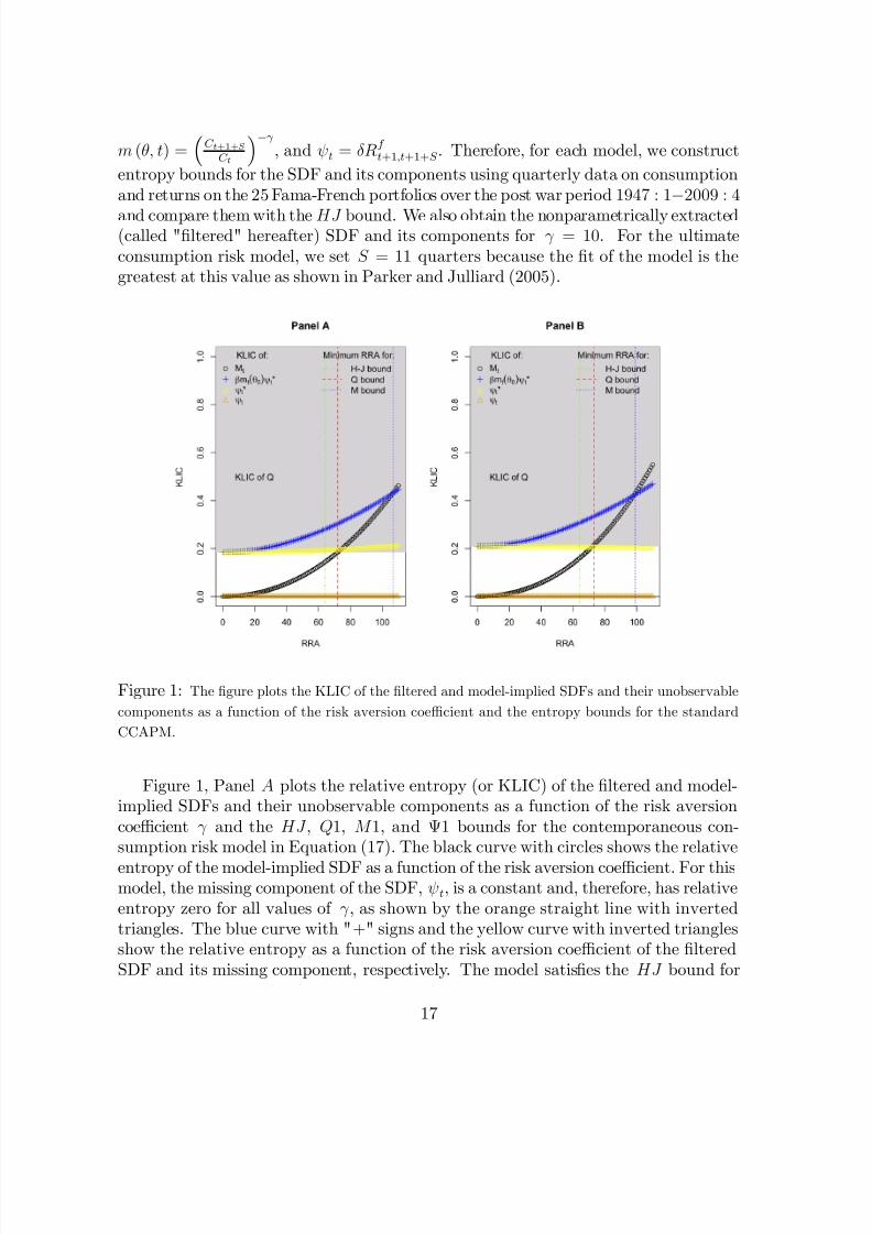
entropy bounds for the SDF and its components using quarterly data on consumptionand returns on the 25 Fama-French portfolios over the post war period 1947 : 12009 : 4
and compare them with theHJ bound. We also obtain the nonparametrically extracted(called "…ltered" hereafter) SDF and its components for = 10. For the ultimateconsumption risk model, we set S = 11 quarters because the …t of the model is thegreatest at this value as shown in Parker and Julliard (2005).
Figure 1: The …gure plots the KLIC of the …ltered and model-implied SDFs and their unobservable
components as a function of the risk aversion coe¢cient and the entropy bounds for the standard
CCAPM.
Figure 1, Panel A plots the relative entropy (or KLIC) of the …ltered and model-implied SDFs and their unobservable components as a function of the risk aversioncoe¢cient and the HJ , Q1, M 1, and 1 bounds for the contemporaneous con-sumption risk model in Equation (17). The black curve with circles shows the relative
entropy of the model-implied SDF as a function of the risk aversion coe¢cient. For thismodel, the missing component of the SDF, t, is a constant and, therefore, has relativeentropy zero for all values of , as shown by the orange straight line with invertedtriangles. The blue curve with "+" signs and the yellow curve with inverted trianglesshow the relative entropy as a function of the risk aversion coe¢cient of the …lteredSDF and its missing component, respectively. The model satis…es the HJ bound for
17

8/4/2019 07 CCAPMmissing No Yogo
http://slidepdf.com/reader/full/07-ccapmmissing-no-yogo 18/43
very high values of > 64, as shown by the green dotted-dashed vertical line. It satis-…es the Q1 bound for even higher values of > 72, as shown by the red dashed verticalline. The minimum value of at which the M 1 bound is satis…ed is given by the value
corresponding to the intersection of the black and blue curves, i.e. it is the minimumvalue of for which the relative entropy of the model-implied SDF exceeds that of the…ltered SDF. The …gure shows that this corresponds to = 107. Finally, the 1 boundis the minimum value of for which the missing component of the model-implied SDFhas a higher relative entropy than the missing component of the …ltered SDF. Sincethe former has zero relative entropy while the latter has a strictly positive value for allvalues of , the model fails to satisfy the 1 bound for any value of . That is, all thebounds reject the model for low RRA even though the best …tting level for the RRAcoe¢cient is smaller than 10 ( = 1:5) and at this value of the coe¢cient the model isable to explain about 60% of the cross-sectional variation across the 25 Fama-Frenchportfolios.
Panel B shows that very similar results are obtained for the Q2, M 2, and 2bounds. The Q2 and M 2 bounds are satis…ed for values of at least as large as 73and 99, respectively, while the 2 bound is not satis…ed for any value of . Overall, assuggested by the theoretical predictions, the Q-bounds are tighter than the HJ -bound,the M -bounds are tighter than the Q-bounds, and the -bounds are tighter than theM -bounds.
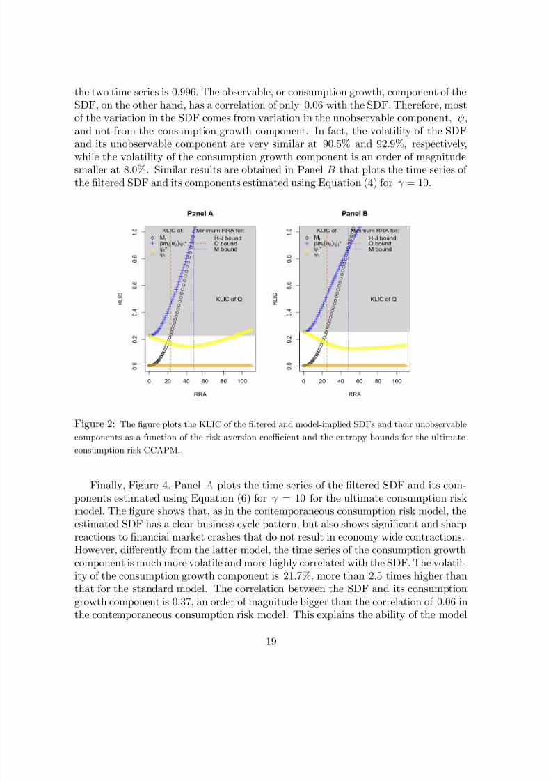
Figure 2 presents analogous results to Figure 1 for the ultimate consumption riskmodel in Equation (18). Panel A shows that the HJ , Q1, and M 1 bounds are satis…edfor > 22, 23, and 46, respectively. These are almost three times, more than threetimes, and more than two times smaller, respectively, than the corresponding values inFigure 1, Panel A for the contemporaneous consumption risk model. As for the lattermodel, the 1 bound is not satis…ed for any value of . Panel B shows that the Q2and M 2 bounds are satis…ed for > 24 and 47, respectively, while the 2 bound isnot satis…ed for any value of .
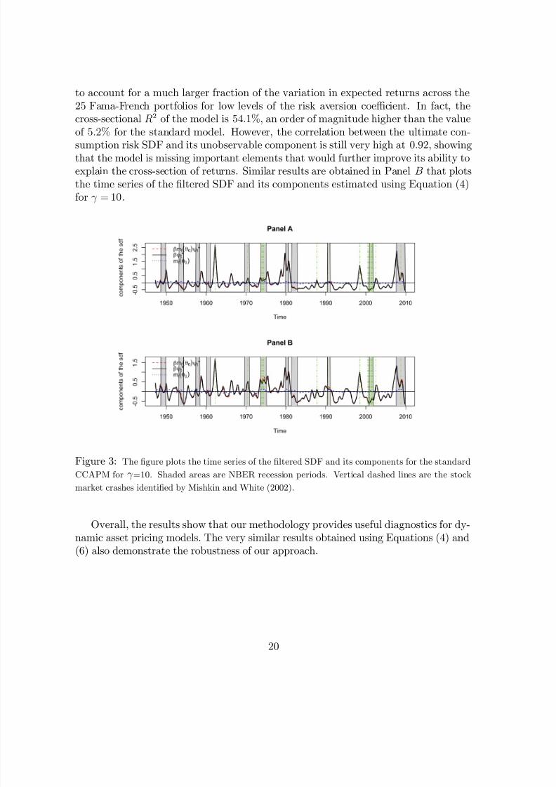
Figure 3, Panel A plots the time series of the …ltered SDF and its componentsestimated using Equation (6) for = 10 for the contemporaneous consumption riskmodel. The blue dotted line plots the component of the SDF that is a parametric
function of consumption growth, m (; t) =
C tC t1
. The red dashed line plots the
…ltered unobservable component of the SDF, t , estimated using Equation (6). The
black solid line plots the …ltered SDF, M t =
C t
C t1
t . The grey shaded areas
represent NBER-dated recessions while the green dashed vertical lines correspond tothe major stock market crashes identi…ed in Mishkin and White (2002). The …gurereveals two main points. First, the estimated SDF has a clear business cycle pattern,but also shows signi…cant and sharp reactions to …nancial market crashes that donot result in economy wide contractions. Second, the time series of the SDF almostcoincides with that of the unobservable component. In fact, the correlation between
18
8/4/2019 07 CCAPMmissing No Yogo
http://slidepdf.com/reader/full/07-ccapmmissing-no-yogo 19/43
the two time series is 0:996. The observable, or consumption growth, component of theSDF, on the other hand, has a correlation of only 0:06 with the SDF. Therefore, mostof the variation in the SDF comes from variation in the unobservable component, ,
and not from the consumption growth component. In fact, the volatility of the SDFand its unobservable component are very similar at 90:5% and 92:9%, respectively,while the volatility of the consumption growth component is an order of magnitudesmaller at 8:0%. Similar results are obtained in Panel B that plots the time series of the …ltered SDF and its components estimated using Equation (4) for = 10.
Figure 2: The …gure plots the KLIC of the …ltered and model-implied SDFs and their unobservable
components as a function of the risk aversion coe¢cient and the entropy bounds for the ultimate
consumption risk CCAPM.
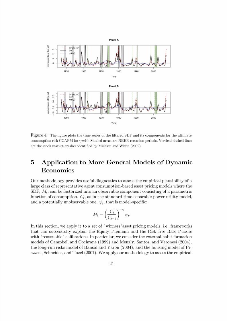
Finally, Figure 4, Panel A plots the time series of the …ltered SDF and its com-ponents estimated using Equation (6) for = 10 for the ultimate consumption riskmodel. The …gure shows that, as in the contemporaneous consumption risk model, theestimated SDF has a clear business cycle pattern, but also shows signi…cant and sharpreactions to …nancial market crashes that do not result in economy wide contractions.
However, di¤erently from the latter model, the time series of the consumption growthcomponent is much more volatile and more highly correlated with the SDF. The volatil-ity of the consumption growth component is 21:7%, more than 2:5 times higher thanthat for the standard model. The correlation between the SDF and its consumptiongrowth component is 0:37, an order of magnitude bigger than the correlation of 0:06 inthe contemporaneous consumption risk model. This explains the ability of the model
19
8/4/2019 07 CCAPMmissing No Yogo
http://slidepdf.com/reader/full/07-ccapmmissing-no-yogo 20/43
to account for a much larger fraction of the variation in expected returns across the25 Fama-French portfolios for low levels of the risk aversion coe¢cient. In fact, thecross-sectional R2 of the model is 54:1%, an order of magnitude higher than the value
of 5:2% for the standard model. However, the correlation between the ultimate con-sumption risk SDF and its unobservable component is still very high at 0:92, showingthat the model is missing important elements that would further improve its ability toexplain the cross-section of returns. Similar results are obtained in Panel B that plotsthe time series of the …ltered SDF and its components estimated using Equation (4)for = 10.
Figure 3: The …gure plots the time series of the …ltered SDF and its components for the standard
CCAPM for =10. Shaded areas are NBER recession periods. Vertical dashed lines are the stock
market crashes identi…ed by Mishkin and White (2002).
Overall, the results show that our methodology provides useful diagnostics for dy-namic asset pricing models. The very similar results obtained using Equations (4) and
(6) also demonstrate the robustness of our approach.
20
8/4/2019 07 CCAPMmissing No Yogo
http://slidepdf.com/reader/full/07-ccapmmissing-no-yogo 21/43
Figure 4: The …gure plots the time series of the …ltered SDF and its components for the ultimate
consumption risk CCAPM for =10. Shaded areas are NBER recession periods. Vertical dashed lines
are the stock market crashes identi…ed by Mishkin and White (2002).
5 Application to More General Models of Dynamic
Economies
Our methodology provides useful diagnostics to assess the empirical plausibility of alarge class of representative agent consumption-based asset pricing models where theSDF, M t, can be factorized into an observable component consisting of a parametricfunction of consumption, C t, as in the standard time-separable power utility model,and a potentially unobservable one, t, that is model-speci…c:
M t =
C tC t1
t.
In this section, we apply it to a set of "winners"asset pricing models, i.e. frameworksthat can successfully explain the Equity Premium and the Risk free Rate Puzzleswith "reasonable" calibrations. In particular, we consider the external habit formationmodels of Campbell and Cochrane (1999) and Menzly, Santos, and Veronesi (2004),the long-run risks model of Bansal and Yaron (2004), and the housing model of Pi-azzesi, Schneider, and Tuzel (2007). We apply our methodology to assess the empirical
21

8/4/2019 07 CCAPMmissing No Yogo
http://slidepdf.com/reader/full/07-ccapmmissing-no-yogo 22/43
plausibility of these models in two ways. First, for each model we compute the valuesof the power coe¢cient, , at which the model-implied SDF satis…es the HJ , Q, M ,and bounds. To simplify the exposition, we focus on one-dimensional bounds as a
function of the risk aversion parameter, , while …xing the other parameters at theauthors’ preferred values. We show that, as suggested by the theoretical predictions,the Q-bounds are generally tighter than the HJ -bound, and the M -bounds are alwaystighter than both HJ and Q bounds. Second, since our methodology identi…es themost likely time-series of the SDF, we compare this time-series with the model-impliedtime-series of the SDF for each model.
In the next Sub-Section we present the models considered. The reader familiar withthese models, can go directly to Section 5.2 without loss of continuity.
5.1 The Models Considered
5.1.1 External Habit Formation Model: Campbell and Cochrane (1999)
In this model, identical agents maximize power utility de…ned over the di¤erence be-tween consumption and a slow-moving habit or time-varying subsistence level. TheSDF is given by
M t =
C tC t1
S tS t1
,
where is the subjective time discount factor, is the curvature parameter, andS t = C tX t
C tdenotes the surplus consumption ratio. Taking logs we have
ln(M t) = ln( ) ct st, (19)
where lower case letters denote the natural logarithms of the upper case letters. There-fore, in this model, the expression for ln(t) is given by:
ln(t) = ln( ) st. (20)
Note that the missing component, , depends on the surplus consumption ratio, S ,that is not observed. To obtain the time series of , we extract the surplus consump-tion ratio from observed consumption data as follows. In this model, the aggregateconsumption growth is assumed to follow an i:i:d: process:
ct = g + t, t i:i:d:N 0; 2 .The log surplus consumption ratio evolves as a heteroskedastic AR(1) process:
st = (1 ) s+ st1 + (st1) t, (21)
22

8/4/2019 07 CCAPMmissing No Yogo
http://slidepdf.com/reader/full/07-ccapmmissing-no-yogo 23/43
where
S =
r
1 ;
(st) = 1
S p 1 2 (st s), if st smax,
0; if st > smax,,
smax = s+1
2
1 S
2
.
For each value of , we use the calibrated values of the model parameters ( , g, , )in Campbell and Cochrane (1999) and the innovations in real consumption growth, bt = ctct1
g , to extract the time series of the surplus consumption ratio using Equation
(21) and, therefore, obtain the time series of the model-implied SDF and its missingcomponent from Equations (19) and (20), respectively.
5.1.2 External Habit Formation Model: Menzly, Santos, and Veronesi(2004)
In this model, the SDF and its missing component are analogous to those in theCampbell and Cochrane (1999) model. The aggregate consumption growth is alsoassumed to follow an i:i:d: process:
dct = cdt+ cdBt,
where c is the mean consumption growth, c > 0 is a scalar, and Bt is a Brownianmotion. The point of departure from the Campbell and Cochrane (1999) model is that
the Menzly, Santos, and Veronesi (2004) model assumes that the inverse surplus, Y t =1S t
, follows a mean reverting process, perfectly negatively correlated with innovationsin consumption growth:
dY t = kY Y tdt (Y t ) [dct E (dct)] , (22)
where Y is the long run mean of the inverse surplus and k is the speed of the meanreversion. For each value of , we use the calibrated values of the model parameters , c, c, k, Y , ,
in Menzly, Santos, and Veronesi (2004) and the innovations in
real consumption growth,
ddBt = [dctE (dct)]
c, to extract the time series of the surplus
consumption ratio and, therefore, obtain the time series of the model-implied SDF andits missing component from Equations (19) and (20), respectively.
5.1.3 Long-Run Risks Model: Bansal and Yaron (2004)
The Bansal and Yaron (2004) long-run risks model assumes that the representativeconsumer has the version of Kreps and Porteus (1978) preferences adopted by Epstein
23
8/4/2019 07 CCAPMmissing No Yogo
http://slidepdf.com/reader/full/07-ccapmmissing-no-yogo 24/43
and Zin (1989) and Weil (1989) for which the SDF is given by
lnM t+1 = log
ct+1 + ( 1)rc;t+1, (23)
where rc;t+1 is the unobservable log gross return on an asset that delivers aggregateconsumption as its dividend each period, is the subjective time discount factor, is the elasticity of intertemporal substitution, = 1
1 1
, and is the risk aversion
coe¢cient.The aggregate consumption and dividend growth rates, ct+1 and dt+1, respec-
tively, are modeled as containing a small persistent expected growth rate component,xt, and ‡uctuating variance, t:
xt+1 = xxt + 'etzx;t+1,
2t+1
= (1 )2 + 2t
+ wz;t+1
,
ct+1 = c + xt + tzc;t+1,
dt+1 = d + xt + 'dtzd;t+1. (24)
The shocks zx;t+1, z;t+1, zc;t+1, and zd;t+1 are assumed to be i:i:d: N (0; 1) and mutuallyindependent.
For the log-linearized version of the model, the log price-consumption ratio, zt, thelog price-dividend ratio, zm;t, and the log risk free rate are a¢ne functions of the statevariables, xt and 2t ,
zt = A0 +A1xt +A22t , (25)
zm;t = A0;m +A1;mxt +A2;m2t , (26)rf;t = A0;f +A1;f xt +A2;f
2t . (27)
Constantinides and Ghosh (2010) argue that Equations (26) and (27) express theobservable variables, zm;t and rf;t, as a¢ne functions of the latent state variables, xtand 2t . Therefore, these Equations may be inverted to express the unobservable statevariables, xt and 2t , in terms of the observables, zm;t and rf;t.
Now, substituting the log-a¢ne approximation for rc;t+1 = 0 + 1zm;t+1 zm;t +ct+1 into the expression for the pricing kernel (Equation (23)), and noting that zt isgiven by Equation (25), we have,
lnM t+1 = ( log + ( 1) [0 + (1 1)A0]) +
+ 1ct+1 (28)
+( 1)1A1xt+1 + ( 1)1A22t+1 ( 1)A1xt ( 1)A2
2t .
Equation (28) for the pricing kernel involves the unobservable (from the point of view of the econometrician) state variables, xt and 2t . Since xt and 2t are a¢ne
24

8/4/2019 07 CCAPMmissing No Yogo
http://slidepdf.com/reader/full/07-ccapmmissing-no-yogo 25/43
functions of zm;t and rf;t, we have,
lnM t+1 = c1 ct+1 + c3rf;t+1 1
1rf;t+ c4zm;t+1
1
1zm;t , (29)
where the parameters c = (c1; c3; c4)0 are functions of the parameters of the time-seriesprocesses and the preference parameters.
The model is calibrated at the monthly frequency. Since we assess the empiricalplausibility of models at the quarterly and annual frequencies, we obtain the pricingkernels at these frequencies by aggregating the monthly kernels. For instance, thequarterly pricing kernel is obtained as
lnM qt+1 =3
Xi=1
lnM t+i
= 3c1 cqt+1 + c3rf;t;t+3 11rf;t;t+2
+c4
zm;t+1 + zm;t+2 + zm;t+3
1
1[zm;t + zm;t+1 + zm;t+2]
. (30)
Therefore, the expression for ln(t) is given by:
ln(t) = 3c1+c3
rf;t;t+3
1
1rf;t;t+2
+c4
zm;t+1 + zm;t+2 + zm;t+3
1
1[zm;t + zm;t+1 + zm;t+2]
,
(31)For each value of , we use the calibrated parameter values from Bansal and Yaron(2004) and the time series of the price-dividend ratio and risk free rate to obtain thetime series of the SDF and its missing component, , in Equations (30) and (31),respectively.
5.1.4 Housing: Piazzesi, Schneider, and Tuzel (2007)
In this model, the pricing kernel is given by:
M t =
C tC t1
1= At
At1
()(1)
,
At =P ct C t
P ct C t + P st S t,
where At is the expenditure share on non-housing consumption, P st and P ct are theprices of housing and non-housing consumption, respectively, and S t and C t are thehousing and non-housing consumption, respectively. is the intertemporal elasticity
25

8/4/2019 07 CCAPMmissing No Yogo
http://slidepdf.com/reader/full/07-ccapmmissing-no-yogo 26/43
of substitution and is the intratemporal elasticity of substitution between housingservices and non-housing consumption.
Taking logs we have:
ln(M t) = ln( ) 1=ct + ( )( 1)
at, (32)
Therefore, in this model, the expression for ln(t) is given by:
ln(t) = ln( ) +( )
( 1)at, (33)
For each value of = 1 , we use the calibrated values of the model parameters ( , )
in Piazzesi, Schneider, and Tuzel (2007) to obtain the time series of the model-impliedSDF and its missing component from Equations (32) and (33), respectively.
5.2 Empirical Results
We apply our methodology to assess the empirical plausibility of the models just de-scribed in two ways. First, for each model we compute the minimum values of thepower coe¢cient, , at which the model-implied SDF satis…es the HJ , Q, M , and bounds. Table 1 reports the results at the quarterly frequency. Panels A, B, C , D,E , and F report results when the set of assets used in the construction of the boundsinclude the market, 25 Fama-French, 10 size-sorted, 10 book-to-market-equity-sorted,10 momentum-sorted, and 10 inductry-sorted portfolios, respectively. Consider …rstthe results for the HJ , Q1, M 1, and 1 bounds. The …rst row in each panel presentsthe bounds for the Campbell and Cochrane (1999) external habit model (henceforthreferred to as CC ). Panel A shows that when the excess return on the market portfoliois used in the construction of the bounds, the minimum value of at which the pricingkernel satis…es the HJ , Q1, M 1, and 1 bounds is 1:4 in all four cases. However, whenthe set of test assets consists of the excess returns on the 25 Fama-French portfolios,Panel B shows that the HJ , Q1, M 1, and 1 bounds are satis…ed for a minimum valueof = 7:3, 9:8, 9:9, and 13:9, respectively. Therefore, as suggested by the theoreticalpredictions, the Q-bound is tighter than the HJ -bound, the M -bound is tighter thanthe Q-bound. Note that in this model, the coe¢cient of risk aversion is
S t, where S t
is the surplus consumption ratio. For = 2, which is the calibrated value from
CC, the risk aversion varies over [20;1). Panel B reveals that the Q-bound issatis…ed for > 9:8, implying that the risk aversion varies over [44:5;1), the M -bound is satis…ed for > 9:9, implying that the risk aversion varies over [43:0;1),and the -bound is satis…ed for > 13:9, implying that the risk aversion varies over[51:5;1). A similar ordering of the bounds is obtained when the set of assets consistof the 10 size-sorted, 10 book-to-market-equity-sorted, 10 momentum-sorted, and 10
26

8/4/2019 07 CCAPMmissing No Yogo
http://slidepdf.com/reader/full/07-ccapmmissing-no-yogo 27/43
industry-sorted portfolios in Panels C , D, E , and F , respectively. Also, very similarresults are obtained for the Q2, M 2, and 2 bounds pointing to the robustness of ourmethodology.
The second row in each panel presents the bounds for the Menzly, Santos, andVeronesi (2004) external habit model (henceforth referred to as MSV ). When the setof test assets consists of the excess return on the market portfolio, the HJ , Q1, M 1,and 1 bounds are satis…ed for a minimum value of = 11:4, 11:2, 12:4, and 15:7,respectively. For the 25 Fama-French portfolios, the bounds are much higher at 27:8,31:7, 33:9, and 53:3, respectively. Therefore, this model requires very high values of the local curvature of the utility function to explain the equity premium and the cross-section of asset returns. In fact, this model requires much higher levels of riskaversion compared to the CC model for each set of test assets. As in the caseof the CC model, very similar results are obtained for the Q2, M 2, and 2 bounds.
The third row in each panel presents the bounds for the Bansal and Yaron (2004)
long run risks model (henceforth referred to as BY ). Panel A shows that when theexcess return on the market portfolio is used in the construction of the bounds, theminimum value of at which the pricing kernel satis…es the HJ , Q1, M 1, and 1bounds is 3:0 in all four cases. When the set of test assets consists of the excess returnson the 25 Fama-French portfolios, Panel B shows that the HJ bound is satis…ed fora minimum value of = 4:0 while the Q1, M 1, and 1 bounds are satis…ed for aminimum value of = 5:0. Similar results are obtained for the other sets of portfoliosand for the Q2, M 2, and 2 bounds. In this model represents the coe¢cient of relative risk aversion. Therefore, the results in Panels A F reveal that the model-implied pricing kernel satis…es the HJ , Q, M , and bounds for reasonable values of the risk aversion coe¢cient for all sets of test assets.
Finally, the fourth row in each panel presents the bounds for the Piazzesi, Schneider,and Tuzel (2007) housing model (henceforth referred to as PST ). When the set of testassets consists of the excess return on the market portfolio, the HJ , Q1 (Q2),M 1 (M 2),and 1 (2) bounds are satis…ed for a minimum value of = 19:2, 19:2(19:4), 24:4(24:3),and 16:2(16:5), respectively. For the 25 Fama-French portfolios, the bounds are muchhigher at 64:3, 75:0(74:5), 87:2(83:8), and 70:9(72:5), respectively. Therefore, thismodel requires very high levels of risk aversion to explain the equity premium and thecross-section of asset returns.
Overall, Table 1 demonstrates that, in line with the theoretical underpinnings of the various bounds, the Q-bound is generally tighter than the HJ -bound because it
naturally exploits the restriction that the SDF is a strictly positive random variable.The M -bound is tighter than the Q-bound because it formally takes into account theability of the SDF to price assets. This relative ordering holds for a variety of di¤erentdynamic asset pricing models. Furthermore, the results suggest that while the externalhabit models of CC and MSV, the housing model of PST require very high levels of riskaversion to satisfy the bounds, the long run risks model of BY satis…es the bounds
27

8/4/2019 07 CCAPMmissing No Yogo
http://slidepdf.com/reader/full/07-ccapmmissing-no-yogo 28/43
for reasonable levels of risk aversion for all sets of test assets.Table 2 reports analogous bounds as in Table 1 at the annual frequency. The
table shows that, at the annual frequency, the HJ , Q, M , and bounds are satis…ed
for much smaller values of the utility curvature parameter, , for each of the modelsconsidered and for each set of test assets. There is also less dispersion between thebounds compared to the quarterly data in Table 1. However, in line with the theoreticalpredictions, the Q-bound is generally tighter than the HJ -bound, and the M -bound isgenerally tighter than the Q-bound.
Our second approach to assessing the empirical plausibility of these models is basedon the observation that our methodology identi…es the most likely time-series of theSDF, which we call the …ltered SDF . We compare the …ltered SDF with each of the model-implied SDFs. Note that the …ltered SDF and its missing componentdepend on the local curvature of the utility function, . Therefore, for each model, we…x at its calibrated value and extract the time series of the SDF and its components.
Table 3 reports the results at the quarterly frequency. In order to examine the models’ability to explain the cross-section of asset returns, we do not consider the marketreturn on its own but focus instead on multiple test assets. Panels A, B, C , D,and E report results for the following sets of test assets: 25 Fama-French, 10 size-sorted, 10 book-to-market-equity-sorted, 10 momentum-sorted, and 10 industry-sortedportfolios, respectively. The …rst column reports the correlation between the …lteredtime series of the missing component, ft gT
t=1, of the SDF and the corresponding
model-implied time series, fmt gT
t=1. The second column shows the correlation between
the …ltered SDF, fM t = mtt gT
t=1, wheremt =
C tC t1
, and the model-implied SDF,
fM mt = mtmt gT
t=1.
Consider …rst the results for the CC external habit model that are presented in the…rst row of each panel. For this model, the utility curvature parameter is set to thecalibrated value of = 2. Panel A, Column 1 shows that when the 25 FF portfolios areused in the extraction of , the correlation between the …ltered and model-implied is only 0:02 when is estimated using Equation (6). Column 2 shows that thecorrelation between the …ltered and model-implied SDFs is marginally higher at 0:05.When is estimated using Equation (4), the correlations are very similar at 0:06 and0:08, respectively. Panels B E show that the correlations between the …ltered andmodel-implied SDFs and their missing components remain small for all the other setsof portfolios.
The second row in each panel presents the results for the MSV external habit model.In this case, is set equal to 1 which is the calibrated value in the model. Row 2 in eachpanel shows that the results for the MSV model are very similar to those for the CCmodel. When is estimated using Equation (6), the correlations between the …lteredand model-implied missing components of the SDFs are small varying from 0:00 forthe 25 FF portfolios to 0:20 for the size-sorted portfolios. The correlations between the
28
8/4/2019 07 CCAPMmissing No Yogo
http://slidepdf.com/reader/full/07-ccapmmissing-no-yogo 29/43
…ltered and model-implied SDFs are marginally higher varying from 0:02 for the 25 FFportfolios to 0:24 for the size-sorted portfolios. Similar results are obtained when isestimated using Equation (4).
The third row in each panel presents the results for the BY long run risks model.Note that the long run risks model implies that the SDF is an exponentially a¢nefunction of the log aggregate consumption growth, the market-wide log price-dividendratio and its lag, and the log risk free rate and its lag (Equation (29)):
lnt+1 = c1 + c3
rf;t+1
1
1rf;t
+ c4
zm;t+1
1
1zm;t
,
lnM t+1 = ct+1 + lnt+1,
where the parameters c = (c1; c3; c4)0 are functions of the underlying model parameters,some of which are not “deep” preference parameters but instead characterizations of the
data generating processes. Since the parameters of the data generating processes couldbe in principle di¤erent in di¤erent samples, we present two types of results for the SDFof the BY model. First, we present results where the restrictions on the parameter, c,implied by the BY calibration are imposed (Row 3). Second, we provide results wherethe parameter vector c is treated as free (in parentheses in Row 3). The parameter is set equal to the BY calibrated value of 10. Row 3, Panel A, Column 1 showsthat when the 25 FF portfolios are used in …ltering the SDF, the correlation betweenthe …ltered and model-implied missing components of the SDFs is 0:10(0:11) when therestrictions are imposed on the coe¢cients c and is estimated using Equation (6)(Equation (4)). This is an order of magnitude higher than the values obtained for theCC and MSV models in Rows 1 and 2, respectively. When the coe¢cients c are treated
as free parameters, the correlation more than doubles from 0:10(0:11) to 0:27(0:29).Column 2 shows that the correlation between the …ltered and model-implied SDFs is0:11(0:12) in the presence of the restrictions and is more than two times higher at0:30(0:31) when the restrictions are not imposed.
Similar results are obtained in Panels B E for the other sets of test assets. Thecorrelation between the …ltered and model-implied missing components of the SDFvaries from 0:12(0:11) for the 10 momentum-sorted portfolios to 0:38(0:38) for the size-sorted portfolios for the restricted speci…cation. These are often an order of magnitudehigher than the correlations obtained for the CC and MSV models. For the unrestrictedspeci…cation, the correlations more than double, varying from 0:44(0:44) for the 10
momentum-sorted portfolios to 0:80(0:82) for the size-sorted portfolios. These resultsshow that the SDF implied by the long run risks model correlates morestrongly with the non-parametrically extracted time series of the SDF thanthe external habit models of CC and MSV.
The fourth row in each panel presents the results for the PST housing model. In thiscase, is set equal to 16 which is the calibrated value in the original paper. Column
29

8/4/2019 07 CCAPMmissing No Yogo
http://slidepdf.com/reader/full/07-ccapmmissing-no-yogo 30/43
1 shows that the correlations between the …ltered and model-implied miss-ing components of the SDFs are very small and often negative, varying from0:22 (0:20) for the size-sorted portfolios to 0:13(0:12) for the industry-sorted portfo-
lios when
is estimated using Equation (6) (Equation (4)). The correlations betweenthe …ltered and model-implied SDFs are marginally higher varying from 0:01 (0:02)for the size-sorted portfolios to 0:19(0:17) for the industry-sorted portfolios.
Table 4 reports analogous results to Table 3 at the annual frequency. Theresults are largely similar to those in Table 3. At the annual frequency, the SDFimplied by the long run risks model correlates more strongly with the …l-tered SDF relative to the external habit and housing models.
The last two columns of Tables 3 and 4 report the cross-sectional R2 implied bythe model SDF for the di¤erent sets of test assets at the quarterly and annual frequen-cies, respectively. The cross-sectional R2 are obtained by performing a cross-sectionalregression of the historical average returns on the model-implied expected returns.
Column 3 reports the cross-sectional R2 when there is no intercept in the regressionwhile Column 4 presents results when an intercept is included. The results reveal thatthe cross-sectional R2 often varies wildly for the same model, and often take on largenegative values when an intercept is not allowed in the cross-sectional regression, whenevaluated using di¤erent sets of assets. This is in stark contrast with the results basedon entropy bounds in Tables 1 and 2, that tend instead to give consistent results foreach model across di¤erent sets of assets (even though all models seem to performbetter, along this dimension, at annual frequency).
A notable exception to the poor cross-sectional performance of the models consid-ered is that, at the annual frequency, the BY model, unlike the CC, MSV, and PSTmodels, has stable cross-sectional R2 for the size and BM-sorted portfolios both in thepresence and absence of an intercept.
Overall, Tables 3 and 4 make two main points. First, they demonstrate the robust-ness of our estimation methodology in that very similar results are obtainedusing Equations (6) and (4). Second, they show that the long run risks model impliesan SDF that is the most highly correlated with the …ltered SDF – the most likely SDFgiven the data.
Tables 5 and 6 report the correlations between the …ltered and model-implied SDFsand the three Fama-French (FF) factors at the quarterly and annual frequencies, re-spectively. Column 1 presents the correlation between the model-implied SDF and thethree FF factors. This is computed by performing a linear regression of the model-
implied time series of the SDF, fM mt g
T
t=1, on the three FF factors and computing thecorrelation between M m and the …tted value from the regression. Similarly, Columns4 and 5 present the correlation of the …ltered SDF and its missing component withthe three FF factors, respectively. These columns provide interesting results becausethe FF factors have been very successful at explaining the cross-sectional variation inreturns between di¤erent classes of …nancial assets.
30
8/4/2019 07 CCAPMmissing No Yogo
http://slidepdf.com/reader/full/07-ccapmmissing-no-yogo 31/43
Consider …rst Table 5. Row 1 of each panel shows that for the CC model, thecorrelation between the model-implied SDF and the three FF factors is small at 0:18.Panel A, Row 1, Column 2 shows that, while the model-implied SDF correlates poorly
with the FF factors, the …ltered SDF correlates very highly with the factors having acorrelation coe¢cient of 0:54 and 0:59 when is estimated using Equations (6) and(4), respectively. This is reassuring for our methodology because, as is well known, theFF factors are successful in explaining a large fraction of the cross-sectional dispersionis asset returns. Moreover, Column 3 reveals that this high correlation is due almostentirely to the missing component, , and not m - the correlation between the …lteredSDF and the FF factors is the same as that between the …ltered missing componentof the SDF and the FF factors. The results in Panels B E are largely similar - the…ltered SDF and its missing component have high correlation with the FF factors forall the di¤erent sets of test assets, varing from 0:52(0:52) for the momentum-sortedportfolios to 0:87(0:89) for the size-sorted portfolios, and the high correlation is almost
entirely due to the missing component
.Row 2 in each panel shows that for the MSV model, the correlation between the
model-implied SDF and the FF factors is small at 0:21. Finally, the …ltered SDFcorrelates strongly with the FF factors which is almost entirely driven by the missingcomponent of the SDF and not the consumption growth component.
Row 3 in each panel shows that for the BY model, the correlation between themodel-implied SDF and the FF factors is 0:45 in the presence of the restrictions. Thisis more than double the correlations obtained for the CC and MSV models. Moreover,the correlation further doubles when the restrictions are not imposed varying from0:87 0:92.
Finally, row 4 in each panel shows that for the PST model, the correlation betweenthe model-implied SDF and the FF factors is very small at 0:07. The …ltered SDF, onthe other hand, correlates strongly with the FF factors which is almost entirely drivenby the missing component of the SDF and not the consumption growth component.
Table 6 reveals that very similar results are obtained at the annual frequency. Tables5 and 6 demonstrate the robustness of our estimation methodology - the …ltered timeseries of the SDF and its missing component is quite robust to the choice of the utilitycurvature parameter and the choice of the set of assets.
6 Conclusion
In this paper, we propose an information-theoretic approach to assess the empiricalplausibility of candidate SDFs for a large class of dynamic asset pricing models. Themodels we consider are characterized by having a pricing kernel that can be factorizedinto an observable and component, consisting in general of a parametric function of consumption, and a potentially unobservable one that is model-speci…c.
31

8/4/2019 07 CCAPMmissing No Yogo
http://slidepdf.com/reader/full/07-ccapmmissing-no-yogo 32/43
Based on this decomposition of the pricing kernel, we provide three major contri-butions. First, we construct a new set of entropy bounds that build upon and improvethe ones suggested in the previous litterature in that a) they naturally impose the non
negativity of the pricing kernel (c.f. Hansen and Jagannathan (1991)), b) they aregenerally thigther and have higher information content (c.f. Hansen and Jagannathan(1991) and Stutzer (1995, 1996)), and c) allow to utilize the information contained ina large cross-section of asset returns (cf. Alvarez and Jermann (2005)).
Second, using a relative entropy minimization approach, we also extract nonpara-metrically the time series of both the SDF and its unobservable component. Given thedata, this methodology identi…es the most likely – in the information theoretic sense
– time series of the SDF and its unobservable component. Applying this methodologyto the data we …nd that the estimated SDF has a clear business cycle pattern, but alsoshows signi…cant and sharp reactions to …nancial market crashes that do not result ineconomy wide contractions.
Third, applying the methodology developed in this paper to a large class of dynamicasset pricing models, we …nd that the external habit models of Campbell and Cochrane(1999) and Menzly, Santos, and Veronesi (2004) and the housing model of Piazzesi,Schneider, and Tuzel (2007) require very high levels of risk aversion to satisfy thebounds while the long run risks model of Bansal and Yaron (2004) satis…es the boundsfor reasonable levels of risk aversion. These results are robust to the choice of testassets used in the construction of the bounds as well as the frequency of the data.Moreover, comparing the non-parametrically extracted SDF with those implied by theabove asset pricing models, we again …nd substantial empirical support for the longrun risks framework.
The methodology developed in this paper is considerably general and may be ap-plied to any model that delivers well-de…ned Euler equations like models with heteroge-nous agents, limited stock market participation, and fragile beliefs, as long as the SDFcan be factorized into an observable component and a potentially unobservable one.
32

8/4/2019 07 CCAPMmissing No Yogo
http://slidepdf.com/reader/full/07-ccapmmissing-no-yogo 33/43
References
Alvarez, F., and U. J. Jermann (2005): “Using Asset Prices to Measure the Per-sistence of the Marginal Utility of Wealth,” Econometrica , 73(6), 1977–2016.
Amemiya, T. (1985): Advanced econometrics / Takeshi Amemiya . Harvard UniversityPress, Cambridge, Mass. :.
Bansal, R., and A. Yaron (2004): “Risks for the Long Run: A Potential Resolutionof Asset Pricing Puzzles,” Journal of Finance , 59(4), 1481–1509.
Breeden, D. T. (1979): “An Intertemporal Asset Pricing Model with StochasticConsumption and Investment Opportunities,” Journal of Financial Economics , 7,265–96.
Breeden, D. T., M. R. Gibbons, and R. H. Litzenberger(1989): “EmpiricalTest of the Consumption-Oriented CAPM,” The Journal of Finance , 44(2), 231–262.
Brown, D. E., and R. L. Smith (1990): “A Correspondance Principle for RelativeEntropy Minimization,” Naval Research Logistics , 37(2).
Brunnermeier, M. K., and C. Julliard (2007): “Money Illusion and HousingFrenzies,” Review of Financial Studies , 20(5).
Campbell, J. Y. (1996): “Understanding Risk and Return,” Journal of Political Economy , 104(2), 298–345.
Campbell, J. Y., and J. H. Cochrane (1999): “By Force of Habit: AConsumption-Based Explanation of Aggregate Stock Market Behavior,” Journal of Political Economy , 107(2), 205–51.
Cochrane, J. H. (1996): “A Cross-Sectional Test of an Investment-Based AssetPricing Model,” Journal of Political Economy , 104(3), 572–621.
Constantinides, G. M., and A. Ghosh (2010): “Asset Pricing Tests with LongRun Risks in Consumption Growth,” Manuscript, University of Chicago.
Csiszar, I. (1975): “I-Divergence Geometry of Probability Distributions and Mini-mization Problems,” Annals of Probability , 3, 146–158.
Hansen, L. P., and R. Jagannathan (1991): “Implications of Security Market Datafor Models of Dynamic Economies,” Journal of Political Economy , 99(2), 225–62.
Hansen, L. P., and T. J. Sargent (2010): “Fragile Beliefs and the Price of Uncer-tainty,” Quantitative Economics , 1(1), 129–162.
33
8/4/2019 07 CCAPMmissing No Yogo
http://slidepdf.com/reader/full/07-ccapmmissing-no-yogo 34/43
Hayashi, F. (2000): Econometrics . Princeton University Press: Princeton.
Jaynes, E. T. (1957a): “Information Theory and Statistical Mechanics,” The Physics Review , 106(4), 620–630.
(1957b): “Information theory and statistical mechanics II,” The Physical Review , 108(2), 171–190.
Kitamura, Y., and M. Stutzer (2002): “Connections between entropic and linearprojections in asset pricing estimation,” Journal of Econometrics , 107(1-2), 159–174.
Lettau, M., and S. Ludvigson (2001): “Resurrecting the (C)CAPM: A Cross-Sectional Test When Risk Premia Are Time-Varying,” Journal of Political Economy ,109, 1238–1286.
Mankiw, N. G., and M. D. Shapiro (1986): “Risk and Return: Consumption BetaVersus Market Beta,” Review of Economics and Statistics , 68, 452–59.
Mehra, R., and E. C. Prescott (1985): “The Equity Premium: A Puzzle,” Journal of Monetary Economics , 15(2), 145–61.
Menzly, L., T. Santos, and P. Veronesi (2004): “Understanding Predictability,”Journal of Political Economy , 112(1), 1–47.
Mishkin, F. S., and E. N. White (2002): “U.S. Stock Market Crashes and Their Af-termath: Implications for Monetary Policy,” NBER Working Papers 8992, NationalBureau of Economic Research, Inc.
Owen, A. B. (1988): “Empirical Likelihood Ratio Con…dence Intervals for a SingleFunctional,” Biometrika , 75(2), 237–249.
(1991): “Empirical Likelihood for Linear Models,” The Annals of Statistics ,19(4), 1725–1747.
(2001): Empirical Likelihood . Chapman and Hall.
Parker, J. A., and C. Julliard (2005): “Consumption Risk and the Cross-Sectionof Expected Returns,” Journal of Political Economy , 113(1).
Piazzesi, M., M. Schneider, and S. Tuzel (2007): “Housing, consumption andasset pricing,” Journal of Financial Economics , 83(3), 531–569.
Rubinstein, M. (1976): “The Valuation of Uncertain Income Streams and the Pricingof Options,” Bell Journal of Economics , 7, 407–25.
34

8/4/2019 07 CCAPMmissing No Yogo
http://slidepdf.com/reader/full/07-ccapmmissing-no-yogo 35/43
Stutzer, M. (1995): “A Bayesian approach to diagnosis of asset pricing models,”Journal of Econometrics , 68(2), 367 – 397.
(1996): “A simple Nonparametric Approach to Derivative Security Valuation,”
Journal of Finance , LI(5), 1633–1652.
Weil, P. (1989): “The Equity Premium Puzzle and the Risk-Free Rate Puzzle,”Journal of Monetary Economics , 24, 401–421.
35

8/4/2019 07 CCAPMmissing No Yogo
http://slidepdf.com/reader/full/07-ccapmmissing-no-yogo 36/43
A Appendix
A.1 Additional Proofs and Propositions
Proof of Proposition 1. In a nut-shell, the proof is a simple variant of Laplace’smethod for approximating integrals. First, note that the Q2-bound criterion can berewritten as
D
M M
jjP
=
Z M ln MdP =
Z M ln M p (M) dM
=
Z M ln
M
K p (M) dM
Z M lnKp (M) dM
=
Z g (M) dM lnK: (34)
Since E p(M) [M] = 1 by construction. Similarly, for the Q1-bound criterion we havethat
D
P jjM M
=
Z ln MdP =
Z ln M p (M) dM
=
Z ln
M
K p (M) dM
Z lnKp (M) dM
=
Z g (M) dM lnK: (35)
since R p (M) dM = 1: Second, since g (M) is always positive by construction for bothbounds, and twice di¤erentiable, we can approximate it around M = as
ln g (M) = ln g0 +@ ln g (M)
@ M
M=
(M ) +1
2
@ 2 ln g (M)
@ M2
M=
(M )2
= ln g0 1
22M(M )2
where in passing from the …rst to the second line I used the fact that @ ln g(M)@ M
M=
= 0
and 2M := @ 2 ln g(M)
@ M2 M=1
is positive by log concavity of g (M). Therefore we
have that
g (M) = g0e 1
22M
(M)2
36

8/4/2019 07 CCAPMmissing No Yogo
http://slidepdf.com/reader/full/07-ccapmmissing-no-yogo 37/43
that is, g (M) is proportional to the kernel of a Normal distribution with mean andvariance 2M. Therefore, replacing this last expression into (35) we have
DM M jjP = Z g0e 1
22
M
(M)2
dM lnK = g0q 22M lnK
= g2
s V ar
M t
M
lnK _
g2M
p V ar (M )
and similarly
D
P jjM M
_g1M
p V ar (M )
Proposition 2 (Asymptotic Distribution of
bt) TBA
Proof. TBA
Proposition 3 (Asymptotic distribution of Q-bounds) TBA
Proof. TBA
Proposition 4 (Asymptotic distribution of M -bounds) TBA
Proof. TBA
Proposition 5 (Asymptotic distribution of -bounds) TBA
Proof. TBA
37
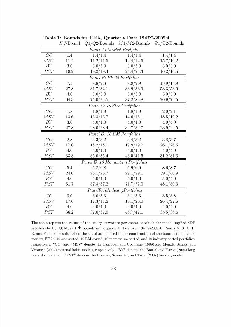
8/4/2019 07 CCAPMmissing No Yogo
http://slidepdf.com/reader/full/07-ccapmmissing-no-yogo 38/43
Table 1: Bounds for RRA, Quarterly Data 1947:2-2009:4HJ -Bound Q1=Q2-Bounds M 1=M 2-Bounds 1=2-Bounds
Panel A: Market Portfolio
CC 1:4 1:4=1:4 1:4=1:4 1:4=1:4MSV 11:4 11:2=11:5 12:4=12:6 15:7=16:2BY 3:0 3:0=3:0 3:0=3:0 3:0=3:0PST 19:2 19:2=19:4 24:4=24:3 16:2=16:5
Panel B: FF 25 Portfolios CC 7:3 9:8=9:8 9:9=9:9 13:9=13:9MSV 27:8 31:7=32:1 33:9=33:9 53:3=53:9BY 4:0 5:0=5:0 5:0=5:0 5:0=5:0PST 64:3 75:0=74:5 87:2=83:8 70:9=72:5
Panel C: 10 Size Portfolios CC 1:8 1:8=1:9 1:8=1:9 2:0=2:1MSV 13:6 13:3=13:7 14:6=15:1 18:5=19:2BY 3:0 4:0=4:0 4:0=4:0 4:0=4:0PST 27:8 28:0=28:4 34:7=34:7 23:9=24:5
Panel D: 10 BM Portfolios CC 2:8 3:3=3:2 3:4=3:2 3:8=3:7MSV 17:0 18:2=18:1 19:9=19:7 26:1=26:5BY 4:0 4:0=4:0 4:0=4:0 4:0=4:0PST 33:3 36:0=35:4 43:5=41:5 31:2=31:3
Panel E: 10 Momentum Portfolios CC 5:4 6:8=6:8 6:9=6:9 8:6=8:7
MSV 24:0 26:1=26:7 29:1=29:1 39:1=40:9BY 4:0 5:0=4:0 5:0=4:0 5:0=4:0PST 51:7 57:3=57:2 71:7=72:0 48:1=50:3
PanelF:10IndustryPortfolios CC 3:0 3:0=3:3 3:1=3:3 3:5=3:8MSV 17:6 17:3=18:2 19:1=20:0 26:4=27:6BY 4:0 4:0=4:0 4:0=4:0 4:0=4:0PST 36:2 37:0=37:9 46:7=47:1 35:5=36:6
The table reports the values of the utility curvature parameter at which the model-implied SDF
satis…es the HJ, Q, M, and bounds using quarterly data over 1947:2-2009:4. Panels A, B, C, D,E, and F report results when the set of assets used in the construction of the bounds include the
market, FF 25, 10 size-sorted, 10 BM-sorted, 10 momentum-sorted, and 10 industry-sorted portfolios,
respectively. "CC" and "MSV" denote the Campbell and Cochrane (1999) and Menzly, Santos, and
Veronesi (2004) external habit models, respectively. "BY" denotes the Bansal and Yaron (2004) long
run risks model and "PST" denotes the Piazzesi, Schneider, and Tuzel (2007) housing model.
38
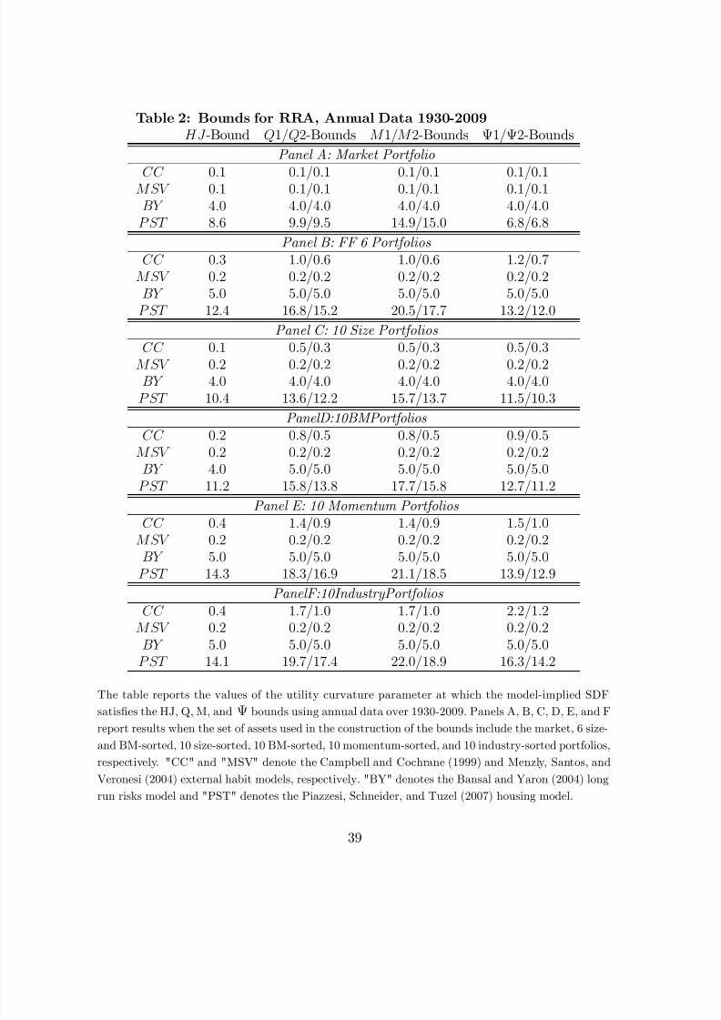
8/4/2019 07 CCAPMmissing No Yogo
http://slidepdf.com/reader/full/07-ccapmmissing-no-yogo 39/43
Table 2: Bounds for RRA, Annual Data 1930-2009HJ -Bound Q1=Q2-Bounds M 1=M 2-Bounds 1=2-Bounds
Panel A: Market Portfolio
CC 0:1 0:1=0:1 0:1=0:1 0:1=0:1MSV 0:1 0:1=0:1 0:1=0:1 0:1=0:1BY 4:0 4:0=4:0 4:0=4:0 4:0=4:0PST 8:6 9:9=9:5 14:9=15:0 6:8=6:8
Panel B: FF 6 Portfolios CC 0:3 1:0=0:6 1:0=0:6 1:2=0:7MSV 0:2 0:2=0:2 0:2=0:2 0:2=0:2BY 5:0 5:0=5:0 5:0=5:0 5:0=5:0PST 12:4 16:8=15:2 20:5=17:7 13:2=12:0
Panel C: 10 Size Portfolios CC 0:1 0:5=0:3 0:5=0:3 0:5=0:3MSV 0:2 0:2=0:2 0:2=0:2 0:2=0:2BY 4:0 4:0=4:0 4:0=4:0 4:0=4:0PST 10:4 13:6=12:2 15:7=13:7 11:5=10:3
PanelD:10BMPortfolios CC 0:2 0:8=0:5 0:8=0:5 0:9=0:5MSV 0:2 0:2=0:2 0:2=0:2 0:2=0:2BY 4:0 5:0=5:0 5:0=5:0 5:0=5:0PST 11:2 15:8=13:8 17:7=15:8 12:7=11:2
Panel E: 10 Momentum Portfolios CC 0:4 1:4=0:9 1:4=0:9 1:5=1:0
MSV 0:2 0:2=0:2 0:2=0:2 0:2=0:2BY 5:0 5:0=5:0 5:0=5:0 5:0=5:0PST 14:3 18:3=16:9 21:1=18:5 13:9=12:9
PanelF:10IndustryPortfolios CC 0:4 1:7=1:0 1:7=1:0 2:2=1:2MSV 0:2 0:2=0:2 0:2=0:2 0:2=0:2BY 5:0 5:0=5:0 5:0=5:0 5:0=5:0PST 14:1 19:7=17:4 22:0=18:9 16:3=14:2
The table reports the values of the utility curvature parameter at which the model-implied SDF
satis…es the HJ, Q, M, and bounds using annual data over 1930-2009. Panels A, B, C, D, E, and Freport results when the set of assets used in the construction of the bounds include the market, 6 size-
and BM-sorted, 10 size-sorted, 10 BM-sorted, 10 momentum-sorted, and 10 industry-sorted portfolios,
respectively. "CC" and "MSV" denote the Campbell and Cochrane (1999) and Menzly, Santos, and
Veronesi (2004) external habit models, respectively. "BY" denotes the Bansal and Yaron (2004) long
run risks model and "PST" denotes the Piazzesi, Schneider, and Tuzel (2007) housing model.
39
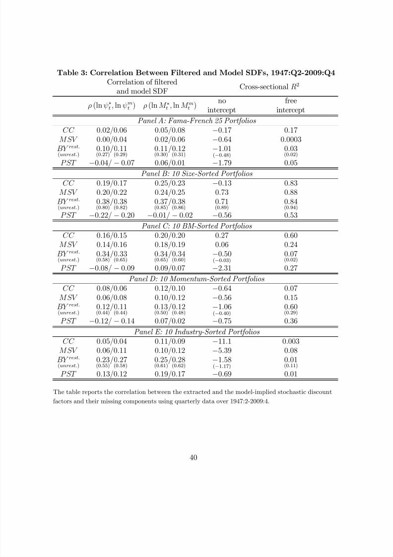
8/4/2019 07 CCAPMmissing No Yogo
http://slidepdf.com/reader/full/07-ccapmmissing-no-yogo 40/43
Table 3: Correlation Between Filtered and Model SDFs, 1947:Q2-2009:Q4Correlation of …ltered
and model SDFCross-sectional R2
(lnt ; lnmt ) (lnM t ; lnM
mt )
nointercept
freeintercept
Panel A: Fama-French 25 Portfolios CC 0:02=0:06 0:05=0:08 0:17 0:17MSV 0:00=0:04 0:02=0:06 0:64 0:0003BY rest:(unrest:)
0:10(0:27)
/0:11(0:29)
0:11(0:30)
/0:12(0:31)
1:01(0:48)
0:03(0:02)
PST 0:04= 0:07 0:06=0:01 1:79 0:05
Panel B: 10 Size-Sorted Portfolios CC 0:19=0:17 0:25=0:23 0:13 0:83
MSV 0:20=0:22 0:24=0:25 0:73 0:88BY rest:(unrest:)
0:38(0:80)
/0:38(0:82)
0:37(0:85)
/0:38(0:86)
0:71(0:89)
0:84(0:94)
PST 0:22= 0:20 0:01= 0:02 0:56 0:53
Panel C: 10 BM-Sorted Portfolios CC 0:16=0:15 0:20=0:20 0:27 0:60MSV 0:14=0:16 0:18=0:19 0:06 0:24BY rest:(unrest:)
0:34(0:58)
/0:33(0:65)
0:34(0:65)
/0:34(0:60)
0:50(0:03)
0:07(0:02)
PST 0:08= 0:09 0:09=0:07 2:31 0:27
Panel D: 10 Momentum-Sorted Portfolios CC 0:08=0:06 0:12=0:10 0:64 0:07MSV 0:06=0:08 0:10=0:12 0:56 0:15BY rest:(unrest:)
0:12(0:44)
/0:11(0:44)
0:13(0:50)
/0:12(0:48)
1:06(0:40)
0:60(0:29)
PST 0:12= 0:14 0:07=0:02 0:75 0:36
Panel E: 10 Industry-Sorted Portfolios CC 0:05=0:04 0:11=0:09 11:1 0:003MSV 0:06=0:11 0:10=0:12 5:39 0:08BY rest:(unrest:)
0:23(0:55)
/0:27(0:58)
0:25(0:61)
/0:28(0:62)
1:58(1:17)
0:01(0:11)
PST 0:13=0:12 0:19=0:17 0:69 0:01
The table reports the correlation between the extracted and the model-implied stochastic discountfactors and their missing components using quarterly data over 1947:2-2009:4.
40
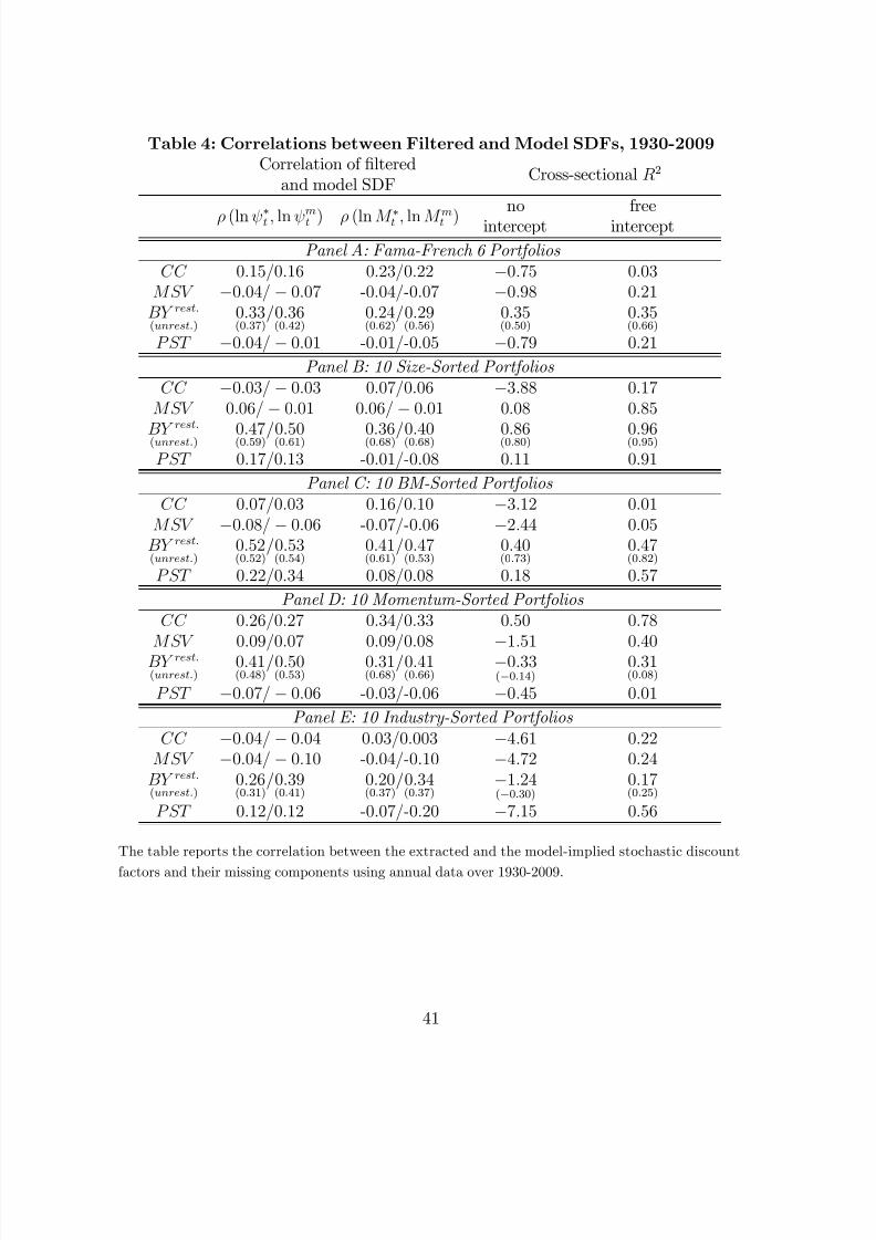
8/4/2019 07 CCAPMmissing No Yogo
http://slidepdf.com/reader/full/07-ccapmmissing-no-yogo 41/43
Table 4: Correlations between Filtered and Model SDFs, 1930-2009Correlation of …ltered
and model SDFCross-sectional R2
(lnt ; ln
mt ) (lnM t ; lnM mt )
nointercept
freeintercept
Panel A: Fama-French 6 Portfolios CC 0:15=0:16 0:23=0:22 0:75 0:03MSV 0:04= 0:07 -0:04=-0:07 0:98 0:21BY rest:(unrest:)
0:33(0:37)
/0:36(0:42)
0:24(0:62)
/0:29(0:56)
0:35(0:50)
0:35(0:66)
PST 0:04= 0:01 -0:01=-0:05 0:79 0:21
Panel B: 10 Size-Sorted Portfolios CC 0:03= 0:03 0:07=0:06 3:88 0:17MSV 0:06= 0:01 0:06= 0:01 0:08 0:85
BY rest:
(unrest:) 0:47(0:59)/0:50(0:61) 0:36(0:68)/0:40(0:68) 0:86(0:80) 0:96(0:95)
PST 0:17=0:13 -0:01=-0:08 0:11 0:91
Panel C: 10 BM-Sorted Portfolios CC 0:07=0:03 0:16=0:10 3:12 0:01MSV 0:08= 0:06 -0:07=-0:06 2:44 0:05BY rest:(unrest:)
0:52(0:52)
/0:53(0:54)
0:41(0:61)
/0:47(0:53)
0:40(0:73)
0:47(0:82)
PST 0:22=0:34 0:08=0:08 0:18 0:57
Panel D: 10 Momentum-Sorted Portfolios CC 0:26=0:27 0:34=0:33 0:50 0:78MSV 0:09=0:07 0:09=0:08 1:51 0:40BY rest:(unrest:)
0:41(0:48)
/0:50(0:53)
0:31(0:68)
/0:41(0:66)
0:33(0:14)
0:31(0:08)
PST 0:07= 0:06 -0:03=-0:06 0:45 0:01
Panel E: 10 Industry-Sorted Portfolios CC 0:04= 0:04 0:03=0:003 4:61 0:22MSV 0:04= 0:10 -0:04=-0:10 4:72 0:24BY rest:(unrest:)
0:26(0:31)
/0:39(0:41)
0:20(0:37)
/0:34(0:37)
1:24(0:30)
0:17(0:25)
PST 0:12=0:12 -0:07=-0:20 7:15 0:56
The table reports the correlation between the extracted and the model-implied stochastic discount
factors and their missing components using annual data over 1930-2009.
41
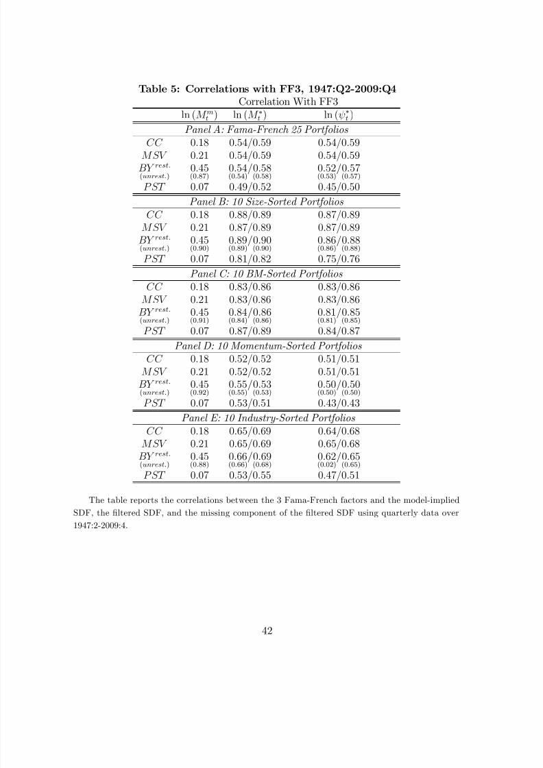
8/4/2019 07 CCAPMmissing No Yogo
http://slidepdf.com/reader/full/07-ccapmmissing-no-yogo 42/43
Table 5: Correlations with FF3, 1947:Q2-2009:Q4Correlation With FF3
ln (M mt ) ln (M t ) ln (t )
Panel A: Fama-French 25 Portfolios CC 0:18 0:54=0:59 0:54=0:59MSV 0:21 0:54=0:59 0:54=0:59BY rest:(unrest:)
0:45(0:87)
0:54(0:54)
/0:58(0:58)
0:52(0:53)
/0:57(0:57)
PST 0:07 0:49=0:52 0:45=0:50
Panel B: 10 Size-Sorted Portfolios CC 0:18 0:88=0:89 0:87=0:89MSV 0:21 0:87=0:89 0:87=0:89BY rest:(unrest:)
0:45(0:90)
0:89(0:89)
/0:90(0:90)
0:86(0:86)
/0:88(0:88)
PST 0:07 0:81=0:82 0:75=0:76
Panel C: 10 BM-Sorted Portfolios CC 0:18 0:83=0:86 0:83=0:86MSV 0:21 0:83=0:86 0:83=0:86BY rest:(unrest:)
0:45(0:91)
0:84(0:84)
/0:86(0:86)
0:81(0:81)
/0:85(0:85)
PST 0:07 0:87=0:89 0:84=0:87
Panel D: 10 Momentum-Sorted Portfolios CC 0:18 0:52=0:52 0:51=0:51MSV 0:21 0:52=0:52 0:51=0:51BY rest:(unrest:)
0:45(0:92)
0:55(0:55)
/0:53(0:53)
0:50(0:50)
/0:50(0:50)
PST 0:07 0:53=0:51 0:43=0:43Panel E: 10 Industry-Sorted Portfolios
CC 0:18 0:65=0:69 0:64=0:68MSV 0:21 0:65=0:69 0:65=0:68BY rest:(unrest:)
0:45(0:88)
0:66(0:66)
/0:69(0:68)
0:62(0:02)
/0:65(0:65)
PST 0:07 0:53=0:55 0:47=0:51
The table reports the correlations between the 3 Fama-French factors and the model-implied
SDF, the …ltered SDF, and the missing component of the …ltered SDF using quarterly data over
1947:2-2009:4.
42
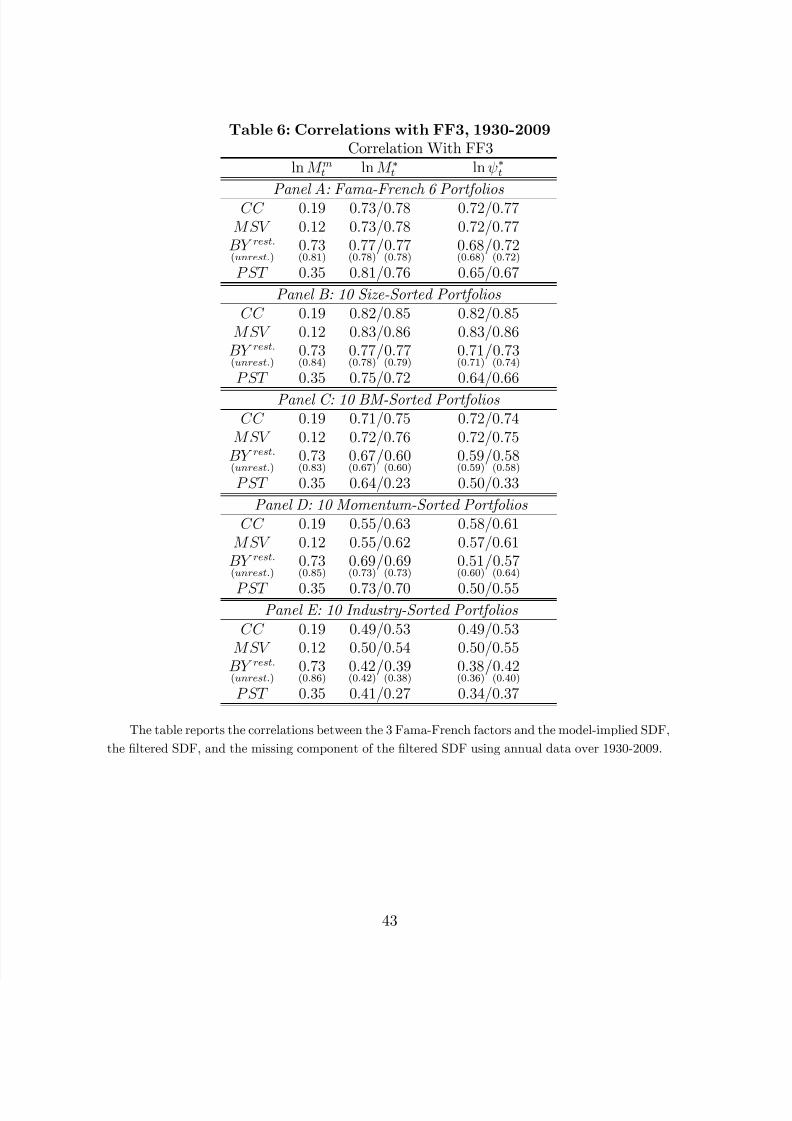
8/4/2019 07 CCAPMmissing No Yogo
http://slidepdf.com/reader/full/07-ccapmmissing-no-yogo 43/43
Table 6: Correlations with FF3, 1930-2009Correlation With FF3
lnM mt lnM t lnt
Panel A: Fama-French 6 Portfolios CC 0:19 0:73=0:78 0:72=0:77MSV 0:12 0:73=0:78 0:72=0:77BY rest:(unrest:)
0:73(0:81)
0:77(0:78)
/0:77(0:78)
0:68(0:68)
/0:72(0:72)
PST 0:35 0:81=0:76 0:65=0:67
Panel B: 10 Size-Sorted Portfolios CC 0:19 0:82=0:85 0:82=0:85MSV 0:12 0:83=0:86 0:83=0:86BY rest:(unrest:)
0:73(0:84)
0:77(0:78)
/0:77(0:79)
0:71(0:71)
/0:73(0:74)
PST 0:35 0:75=0:72 0:64=0:66
Panel C: 10 BM-Sorted Portfolios CC 0:19 0:71=0:75 0:72=0:74MSV 0:12 0:72=0:76 0:72=0:75BY rest:(unrest:)
0:73(0:83)
0:67(0:67)
/0:60(0:60)
0:59(0:59)
/0:58(0:58)
PST 0:35 0:64=0:23 0:50=0:33
Panel D: 10 Momentum-Sorted Portfolios CC 0:19 0:55=0:63 0:58=0:61MSV 0:12 0:55=0:62 0:57=0:61BY rest:(unrest:)
0:73(0:85)
0:69(0:73)
/0:69(0:73)
0:51(0:60)
/0:57(0:64)
PST 0:35 0:73=0:70 0:50=0:55Panel E: 10 Industry-Sorted Portfolios
CC 0:19 0:49=0:53 0:49=0:53MSV 0:12 0:50=0:54 0:50=0:55BY rest:(unrest:)
0:73(0:86)
0:42(0:42)
/0:39(0:38)
0:38(0:36)
/0:42(0:40)
PST 0:35 0:41=0:27 0:34=0:37
The table reports the correlations between the 3 Fama-French factors and the model-implied SDF,
the …ltered SDF, and the missing component of the …ltered SDF using annual data over 1930-2009.
43