Embed Size (px)
Citation preview

Cahier 07-2011
A Model of Dynamic Liquidity Contracts
Onur ÖZGÜR

CIREQ, Université de Montréal C.P. 6128, succursale Centre-ville Montréal (Québec) H3C 3J7 Canada
téléphone : (514) 343-6557 télécopieur : (514) 343-7221 [email protected] http://www.cireq.umontreal.ca
Le Centre interuniversitaire de recherche en économie quantitative (CIREQ) regroupe des chercheurs dans les domaines de l'économétrie, la théorie de la décision, la macroéconomie et les marchés financiers, la microéconomie appliquée et l’économie expérimentale ainsi que l'économie de l'environnement et des ressources naturelles. Ils proviennent principalement des universités de Montréal, McGill et Concordia. Le CIREQ offre un milieu dynamique de recherche en économie quantitative grâce au grand nombre d'activités qu'il organise (séminaires, ateliers, colloques) et de collaborateurs qu'il reçoit chaque année. The Center for Interuniversity Research in Quantitative Economics (CIREQ) regroups researchers in the fields of econometrics, decision theory, macroeconomics and financial markets, applied microeconomics and experimental economics, and environmental and natural resources economics. They come mainly from the Université de Montréal, McGill University and Concordia University. CIREQ offers a dynamic environment of research in quantitative economics thanks to the large number of activities that it organizes (seminars, workshops, conferences) and to the visitors it receives every year.
Cahier 07-2011
A Model of Dynamic Liquidity Contracts
Onur ÖZGÜR

Ce cahier a également été publié par le Département de sciences économiques de l’Université de Montréal sous le numéro (2011-06).
This working paper was also published by the Department of Economics of the University of Montreal under number (2011-06). Dépôt légal - Bibliothèque nationale du Canada, 2011, ISSN 0821-4441 Dépôt légal - Bibliothèque et Archives nationales du Québec, 2011 ISBN-13 : 978-2-89382-616-5
A Model of Dynamic Liquidity Contracts∗
Onur Ozgur†
Universite de Montreal
Department of Economics
December 2010
Abstract
I study long-term financial contracts between lenders and borrowers in the absence of per-
fect enforceability and when both parties are credit constrained. Borrowers repeatedly have
projects to undertake and need external financing. Lenders can commit to contractual agree-
ments whereas borrowers can renege any period. I show that equilibrium contracts feature
interesting dynamics: the economy exhibits efficient investment cycles; absence of perfect en-
forcement and shortage of capital skew the cycles toward states of liquidity drought; credit is
rationed if either the lender has too little capital or if the borrower has too little collateral.
This paper’s technical contribution is its demonstration of the existence and characterization of
financial contracts that are solutions to a non-convex dynamic programming problem.
Journal of Economic Literature Classification Numbers: C6, C7, D9, G2
Keywords: Credit Rationing, credit cycles, default, limited capital, liquidity.
∗I have benefited from conversations with Alberto Bisin and Douglas Gale. I am especially grateful to Douglas Gale
for introducing me to the topic. I also would like to thank Franklin Allen, Adam Ashcraft, Jess Benhabib, Bogachan
Celen, Boyan Jovanovic, Alessandro Lizzeri, Richard McLean, Daniel Quint, Martin Schneider, Til Schuermann,
Adam Szeidl, Ennio Stacchetti, and Jean Tirole for helpful comments, and seminar participants at several universities
and conferences, and at the Bank of England and the Federal Reserve Bank of New York. Part of this research was
done while I was visiting the Economics Department at the Universite Laval. Thanks to Yann Bramoulle and Bernard
Fortin for organizing the visit. I am grateful for financial support to “La Chaire du Canada en Economie des Politiques
Sociales et des Ressources Humaines” at Universite Laval, CIREQ, CIRPEE, IFM2, and FQRSC. Any errors are my
own.†Department of Economics, Universite de Montreal, C.P. 6128, succursale Centre-ville, Montreal, QC H3C 3J7,
Canada; CIREQ, CIRANO; http://www.sceco.umontreal.ca/onurozgur
1

2 Onur Ozgur
1 Introduction
Financial intermediaries are a veil in a standard Arrow-Debreu model. When modeled, in finance,
they are usually taken as deep-pocketed. Empirical evidence tells otherwise as we witnessed recently
during the most damaging financial storm of our lives. Some of the biggest banks, which were
thought to be the untouchables of the finance world, went down stating inability to honor short
term liabilities.1 US government gave in and devised a $700 billion scheme to rescue the financial
system from total collapse. Otherwise more banks were on the line.
About a year later, many capital-injected, too-big-to-fail banks announced solid profits again,
arguably due partly to the changes in the accounting standards used in the valuation of their assets
and partly to the extremely low cost of emergency borrowing from the lenders of last resort2. The
issue is that at times of great economic distress, credit markets freeze and the pricing mechanism
stops working. Transactions are carried out at fire sale prices. The drought of liquidity in the system
halts the well-functioning of the financial intermediaries and consequently that of the economic
system.
This is, of course, not the first time we experience such turmoil. During the credit crunch of
1990, banks started cutting back on lending immensely. Limited bank capital relative to the loan
demand contributed to restrictive bank lending during the recession of 1990/91.3 We know by now
that lender capital has a significant effect on lending and economic activity. As their capital ratios
fall, banks become more conservative in their lending.
The situation is worse for relatively small lenders specializing on local industries and small
firms that depend on small lenders in the form of backing lines of credit and other forms of external
finance. Small firms do not enjoy the same market access and low interest rates as do big ones (see
1On January 29, 2008, Lehman Brothers reported record revenues of nearly $60 billion and record earnings in excess
of $4 billion for the fiscal year 2007. Its stock traded as high as $65.73 per share and averaged in the high to mid-fifties.
Less than eight months later, on September 12, its stock closed under $4, a decline of nearly 95%. On September
15, the once fourth largest investment bank by market capitalization, sought Chapter 11 protection, in the largest
bankruptcy proceeding ever filed (From the Lehman Brothers Holdings Inc. Chapter 11 Proceedings Examiner’s
Report, Jenner&Block, March 2010, New York and Chicago. Available publicly at http://lehmanreport.jenner.com/).2Here is an excerpt from an article in the Financial Times, Markets Section, dated December 3, 2009, on US
banking sector: “A year ago, few people thought the banking sector was the place to be. However, its performance
in the stock market has been nothing short of stellar in 2009.”3See Bernanke and Lown (1991) on the ‘Credit Crunch’. They give anecdotal evidence on Richard Syron, then
president of the Federal Reserve Bank of Boston, calling the crunch a ‘Capital Crunch’. Syron argued in a testimony
before Congress that the credit crunch in New England was due to a shortage in bank capital. Banks in the region
had to write down loans, forced by the real estate bubble, which led to the depletion of their equity capital. In order
to meet regulatory requirements, they had to sell assets and scale down their lending.
Dynamic Liquidity Contracts 3
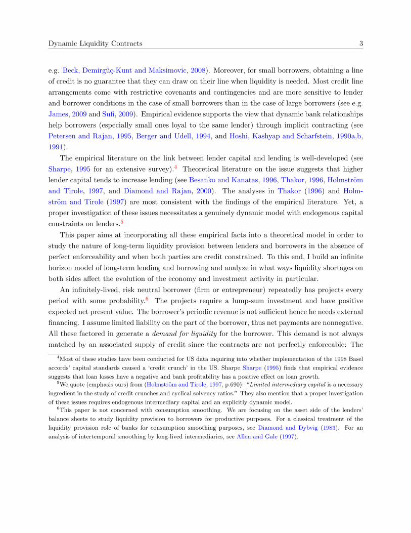
e.g. Beck, Demirguc-Kunt and Maksimovic, 2008). Moreover, for small borrowers, obtaining a line
of credit is no guarantee that they can draw on their line when liquidity is needed. Most credit line
arrangements come with restrictive covenants and contingencies and are more sensitive to lender
and borrower conditions in the case of small borrowers than in the case of large borrowers (see e.g.
James, 2009 and Sufi, 2009). Empirical evidence supports the view that dynamic bank relationships
help borrowers (especially small ones loyal to the same lender) through implicit contracting (see
Petersen and Rajan, 1995, Berger and Udell, 1994, and Hoshi, Kashyap and Scharfstein, 1990a,b,
1991).
The empirical literature on the link between lender capital and lending is well-developed (see
Sharpe, 1995 for an extensive survey).4 Theoretical literature on the issue suggests that higher
lender capital tends to increase lending (see Besanko and Kanatas, 1996, Thakor, 1996, Holmstrom
and Tirole, 1997, and Diamond and Rajan, 2000). The analyses in Thakor (1996) and Holm-
strom and Tirole (1997) are most consistent with the findings of the empirical literature. Yet, a
proper investigation of these issues necessitates a genuinely dynamic model with endogenous capital
constraints on lenders.5
This paper aims at incorporating all these empirical facts into a theoretical model in order to
study the nature of long-term liquidity provision between lenders and borrowers in the absence of
perfect enforceability and when both parties are credit constrained. To this end, I build an infinite
horizon model of long-term lending and borrowing and analyze in what ways liquidity shortages on
both sides affect the evolution of the economy and investment activity in particular.
An infinitely-lived, risk neutral borrower (firm or entrepreneur) repeatedly has projects every
period with some probability.6 The projects require a lump-sum investment and have positive
expected net present value. The borrower’s periodic revenue is not sufficient hence he needs external
financing. I assume limited liability on the part of the borrower, thus net payments are nonnegative.
All these factored in generate a demand for liquidity for the borrower. This demand is not always
matched by an associated supply of credit since the contracts are not perfectly enforceable: The
4Most of these studies have been conducted for US data inquiring into whether implementation of the 1998 Basel
accords’ capital standards caused a ‘credit crunch’ in the US. Sharpe Sharpe (1995) finds that empirical evidence
suggests that loan losses have a negative and bank profitability has a positive effect on loan growth.5We quote (emphasis ours) from (Holmstrom and Tirole, 1997, p.690): “Limited intermediary capital is a necessary
ingredient in the study of credit crunches and cyclical solvency ratios.” They also mention that a proper investigation
of these issues requires endogenous intermediary capital and an explicitly dynamic model.6This paper is not concerned with consumption smoothing. We are focusing on the asset side of the lenders’
balance sheets to study liquidity provision to borrowers for productive purposes. For a classical treatment of the
liquidity provision role of banks for consumption smoothing purposes, see Diamond and Dybvig (1983). For an
analysis of intertemporal smoothing by long-lived intermediaries, see Allen and Gale (1997).
4 Onur Ozgur
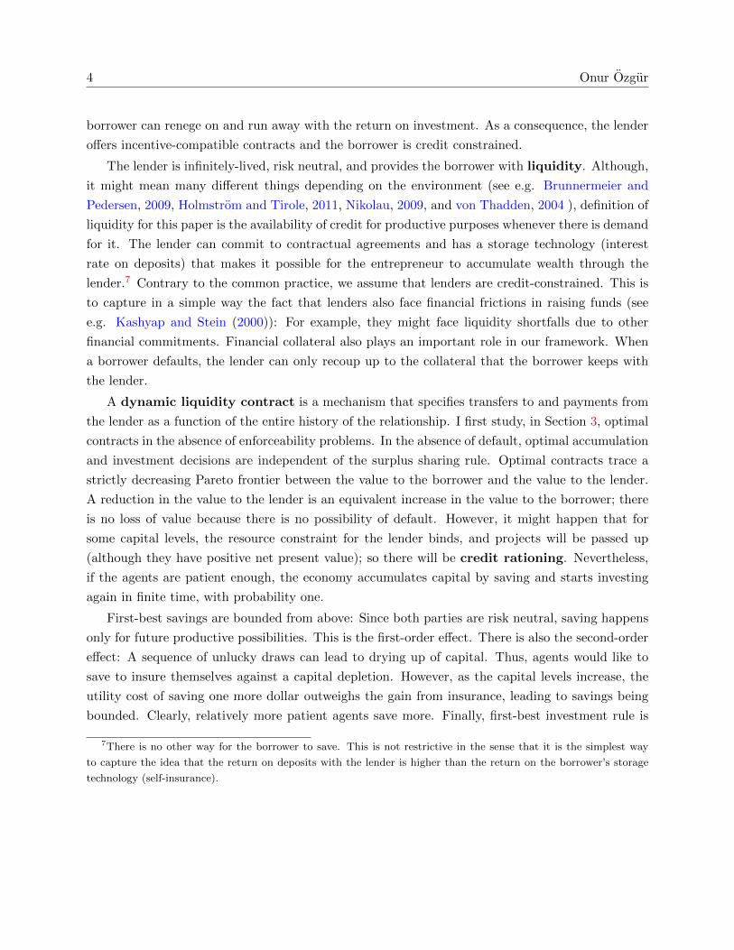
borrower can renege on and run away with the return on investment. As a consequence, the lender
offers incentive-compatible contracts and the borrower is credit constrained.
The lender is infinitely-lived, risk neutral, and provides the borrower with liquidity. Although,
it might mean many different things depending on the environment (see e.g. Brunnermeier and
Pedersen, 2009, Holmstrom and Tirole, 2011, Nikolau, 2009, and von Thadden, 2004 ), definition of
liquidity for this paper is the availability of credit for productive purposes whenever there is demand
for it. The lender can commit to contractual agreements and has a storage technology (interest
rate on deposits) that makes it possible for the entrepreneur to accumulate wealth through the
lender.7 Contrary to the common practice, we assume that lenders are credit-constrained. This is
to capture in a simple way the fact that lenders also face financial frictions in raising funds (see
e.g. Kashyap and Stein (2000)): For example, they might face liquidity shortfalls due to other
financial commitments. Financial collateral also plays an important role in our framework. When
a borrower defaults, the lender can only recoup up to the collateral that the borrower keeps with
the lender.
A dynamic liquidity contract is a mechanism that specifies transfers to and payments from
the lender as a function of the entire history of the relationship. I first study, in Section 3, optimal
contracts in the absence of enforceability problems. In the absence of default, optimal accumulation
and investment decisions are independent of the surplus sharing rule. Optimal contracts trace a
strictly decreasing Pareto frontier between the value to the borrower and the value to the lender.
A reduction in the value to the lender is an equivalent increase in the value to the borrower; there
is no loss of value because there is no possibility of default. However, it might happen that for
some capital levels, the resource constraint for the lender binds, and projects will be passed up
(although they have positive net present value); so there will be credit rationing. Nevertheless,
if the agents are patient enough, the economy accumulates capital by saving and starts investing
again in finite time, with probability one.
First-best savings are bounded from above: Since both parties are risk neutral, saving happens
only for future productive possibilities. This is the first-order effect. There is also the second-order
effect: A sequence of unlucky draws can lead to drying up of capital. Thus, agents would like to
save to insure themselves against a capital depletion. However, as the capital levels increase, the
utility cost of saving one more dollar outweighs the gain from insurance, leading to savings being
bounded. Clearly, relatively more patient agents save more. Finally, first-best investment rule is
7There is no other way for the borrower to save. This is not restrictive in the sense that it is the simplest way
to capture the idea that the return on deposits with the lender is higher than the return on the borrower’s storage
technology (self-insurance).

Dynamic Liquidity Contracts 5
monotonic in the level of capital.
A second-best contract is an incentive-compatible optimal contract. The worst punishment that
can be inflicted upon the borrower in case of default is exclusion from the credit markets. When it
happens, the borrower is left to consume what he expropriated plus his stream of future endowment.
This is a rather standard assumption in the literature on dynamic contracts (see Albuquerque and
Hopenhayn (2004), Alvarez and Jermann (2000), Atkeson (1991), Kehoe and Levine (1993), and
Thomas and Worrall (1994)).8
I then characterize properties of second-best contracts. Enforcement problems and endogenous
resource constraints severely reduce the possibility of financing projects. Investment and savings
are functions both of the level of resources and the surplus sharing rule, in contrast to the first-best
contracts. Investment is (weakly) under-provided. Second-best savings are (weakly) less than first-
best savings capturing the intuition that it does not pay off to postpone consumption/investment
to self-insure against a possible ‘credit crunch’. When agents are relatively patient, they exhibit
investment cycles. For any initial capital level, the economy falls into a ‘credit crunch’ in finite
time, almost surely. With patient agents, this is not an absorbing state. The economy recovers
in the long-run, the capital levels are restored and investment activity goes back to normal, the
lag between a phase of investment and a phase of no-investment gets longer. In economies with
relatively impatient agents, the system gets stuck in that phase and we observe constant stagnation.
If the borrower collateral is too small, the lender might find it too costly to prevent default.
Thus, although the projects have positive net present value, credit might be rationed. This does
not lead to the collapse of the relationship though. As time evolves, the share of the borrower
increases (on average) and credit is extended for the same level of lender capital where initially
credit was rationed. That is because over time borrower rebuilds collateral and holds it with the
lender as a guarantee.
The theoretical structure in the current paper is related to and/or builds upon the literature on
dynamic and relational contracts. See for e.g., Albuquerque and Hopenhayn (2004), Alvarez and
Jermann (2000), Atkeson (1991), Cooley, Marimon, and Quadrini (2004), Hopenhayn and Werning
(2008), Kovrijnykh (2010), Kehoe and Levine (1993), MacLeod and Malcomson (1989), Ray (2002),
and Thomas and Worrall (2010). The paper that comes closest to the current one is Thomas and
Worrall (1994) although there are important distinctions. First of all, theoretically, the current
one is a dynamic game whereas theirs is a repeated game. More importantly, I am interested
in endogenous credit constraints on the part of the lender alongside the by-now more standard
enforceability problems. To the best of my knowledge, the current paper is the first full-blown
8For exceptions see e.g. Cooley, Marimon, and Quadrini (2004) and Phelan Phelan (1995).
6 Onur Ozgur
infinite-horizon dynamic contracting model that allows for “shallow-pocketed” lenders.
Bernanke and Gertler (1989) study an OLG model of business cycle dynamics where borrowers’
balance sheet positions play an important role. They show that agency costs associated with the
undertaking of physical investment are decreasing in the borrower’s net worth, and that this results
in the emergence of accelerator effects on investment. Strengthened balance sheets of borrowers
during good times in turn expand investment demand which tends to amplify the boom; weakened
balance sheets during bad times work in the opposite direction. The same kind of accelerator
effect is exhibited by the dynamics of the second-best contracts in the present paper. However, the
present paper is a full-fledged infinite horizon model of borrowing and lending, internalizing the
gains from long-term relationships. Moreover, in the current paper, unlike Bernanke and Gertler
(1989), cycles can be efficient; i.e., we can observe investment cycles not because of agency costs
but because lender’s capital is scarce and the system enters a ‘capital crunch’.
This paper also contributes a technical analysis of the existence and characterization of optimal
dynamic contracts that are solutions to a non-convex dynamic programming problem. Indivisibil-
ity of the projects along with credit constraints make the set of feasible contracts a non-convex
set. The resulting value functions exhibit discontinuities. The standard methods using concave
programming and/or (super)differentiability of the value functions are not of help. I use a direct
strategy and exploit monotonicity of the resulting operators. The problem of the value function
entering the constraint set was introduced in Thomas and Worrall (1994). In our case, the problem
is exacerbated by the fact that both the borrower and the lender have limited liability constraints
and the continuation values should be nonnegative for both.9 My task is further complicated since,
in game theoretical terms, the problem in their paper is a repeated game whereas the current
problem is a dynamic game with an unbounded state space.
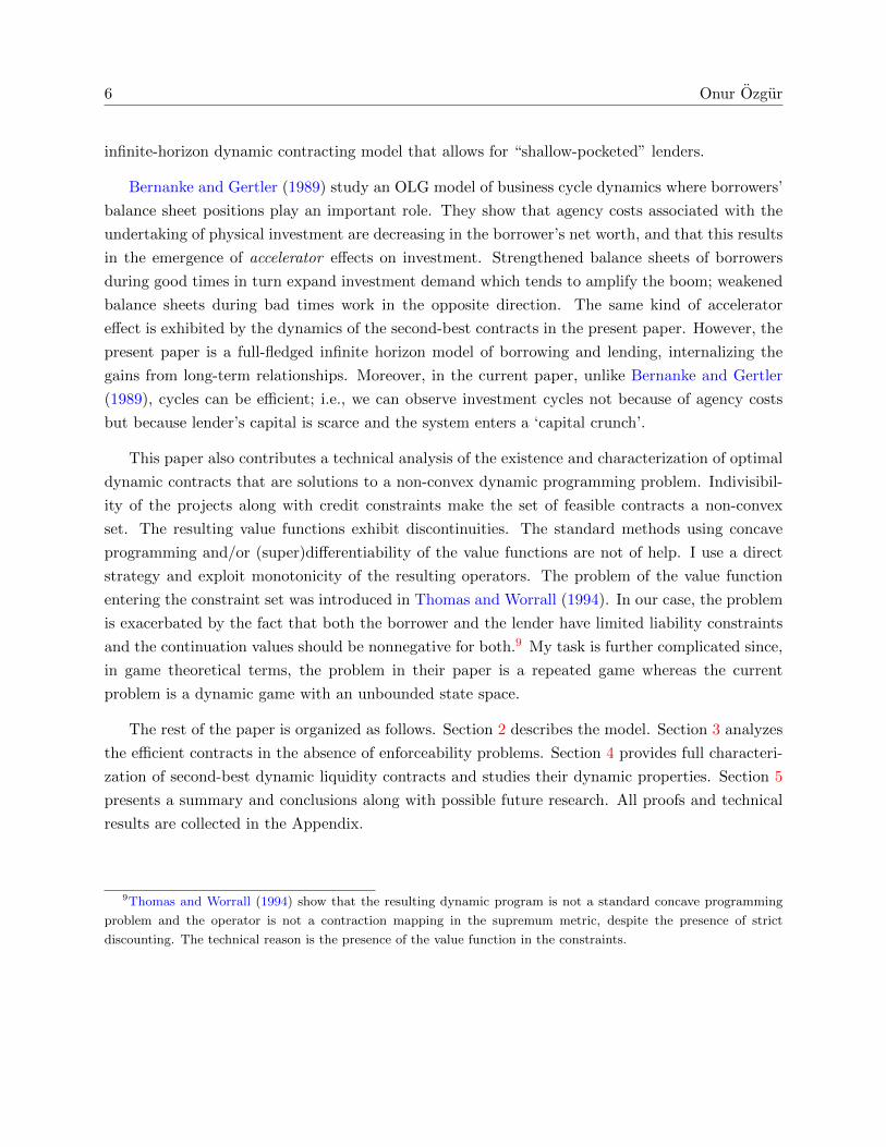
The rest of the paper is organized as follows. Section 2 describes the model. Section 3 analyzes
the efficient contracts in the absence of enforceability problems. Section 4 provides full characteri-
zation of second-best dynamic liquidity contracts and studies their dynamic properties. Section 5
presents a summary and conclusions along with possible future research. All proofs and technical
results are collected in the Appendix.
9Thomas and Worrall (1994) show that the resulting dynamic program is not a standard concave programming
problem and the operator is not a contraction mapping in the supremum metric, despite the presence of strict
discounting. The technical reason is the presence of the value function in the constraints.
Dynamic Liquidity Contracts 7
2 The Model
Time is infinite and is indexed by t = 0, 1, . . .. There are two agents, a borrower (B) and a lender
(L), both infinitely lived. The borrower receives a deterministic endowment of Y > 0 units of the
only consumption good in the economy, every period. Each period, with some probability p ∈ (0, 1),
he has a project that needs to be implemented within that period. Investment requires I > Y units
of the consumption good and generates a verifiable, financial return of D > I units, in the same
period, with probability q, and 0 units with probability (1−q). The net present value of the project
is positive, i.e., qD− I > 0. Let θt be the random variable that takes the value 1 if the agent has a
project at time t (liquidity shock), 0 otherwise. Similarly, let µt be the random variable that takes
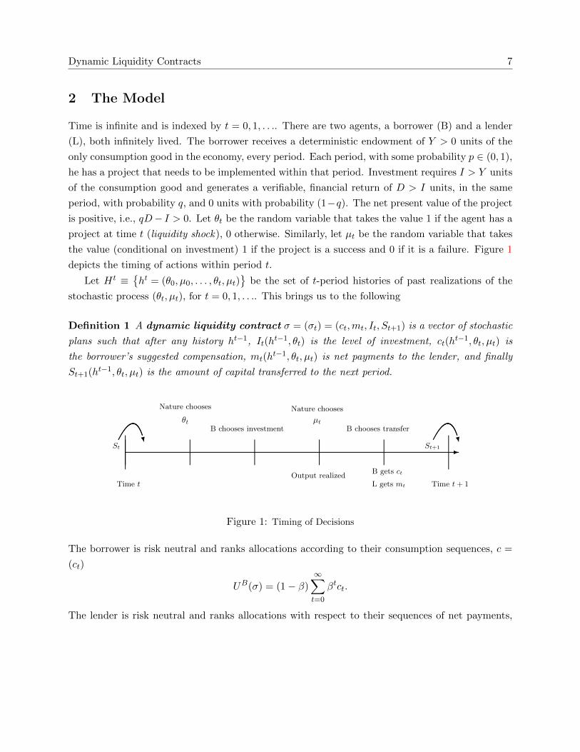
the value (conditional on investment) 1 if the project is a success and 0 if it is a failure. Figure 1
depicts the timing of actions within period t.
Let Ht ≡{ht = (θ0, µ0, . . . , θt, µt)
}be the set of t-period histories of past realizations of the
stochastic process (θt, µt), for t = 0, 1, . . .. This brings us to the following
Definition 1 A dynamic liquidity contract σ = (σt) = (ct,mt, It, St+1) is a vector of stochastic
plans such that after any history ht−1, It(ht−1, θt) is the level of investment, ct(h
t−1, θt, µt) is
the borrower’s suggested compensation, mt(ht−1, θt, µt) is net payments to the lender, and finally
St+1(ht−1, θt, µt) is the amount of capital transferred to the next period.
�
Time t
Nature chooses
θtB chooses investment
Nature chooses
μtB chooses transfer
Time t+ 1
�St
�St+1
B gets ct
L gets mt
Output realized
Figure 1: Timing of Decisions
The borrower is risk neutral and ranks allocations according to their consumption sequences, c =
(ct)
UB(σ) = (1− β)
∞∑
t=0
βtct.
The lender is risk neutral and ranks allocations with respect to their sequences of net payments,

8 Onur Ozgur
m = (mt)
UL(σ) = (1− β)∞∑
t=0
βtmt.
and β ∈ (0, 1) is the common discount factor. I follow the common practice in the repeated games
literature and normalize the utility levels to make them comparable to period utilities.
Assumption 1 (One-sided Strategic Default) The lender honors his promises whereas the
borrower might renege on the current contract at any time. If the borrower chooses to default,
he is excluded from the credit markets forever.
The borrower cannot store goods unless he saves by keeping an account with the lender, who has
a storage technology that returns one unit next period for every unit stored in the current one.10
The endowment stream of the borrower guarantees him Y every period. Thus, the autarkic level
of a borrower who does not enter into a long-term contract is defined as vBaut = Y . The lender has
an initial capital level of S0 ≥ 0 units.
3 First-Best Liquidity Contracts
In this section, I solve for efficient contracts, without default. They constitute the benchmark case
relative to which the welfare costs of allowing strategic default are evaluated. Assuming that the
planner has the same information that the agents have and that there are no incentive problems,
any feasible contract should satisfy ∀t, ∀ht
St+1(ht) ≤ St(ht−1) + Y −mt(h
t)− ct(ht)+D 1{θt=1, µt=1 and It(ht−1,θt)≥I} − It(ht−1, θt) (1)
which is an aggregate feasibility constraint.
The idea that liquidity might be limited is captured by the following two constraints: The
liquidity constraints (or equivalently resource or capital constraints), i.e., for any period t, and
for any history ht,
It(ht−1, θt) ≤ St(ht−1) + Y (2)
and the limited liability constraints (nonnegative net payments)
ct,mt, It, St+1 ≥ 0 (3)
10This is just a normalization. As long as the rate that the bank pays for deposits is lower than the rate it can get
for its funds at the market r where β = 1/1 + r, results are not affected.
Dynamic Liquidity Contracts 9
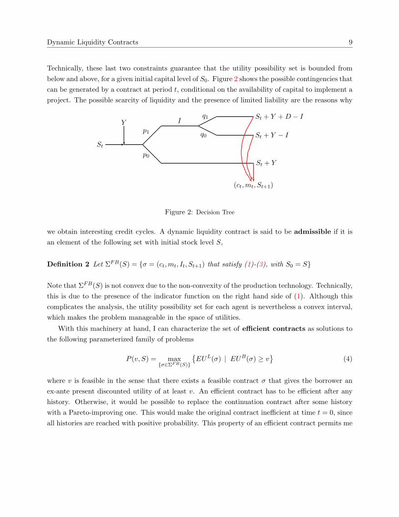
Technically, these last two constraints guarantee that the utility possibility set is bounded from
below and above, for a given initial capital level of S0. Figure 2 shows the possible contingencies that
can be generated by a contract at period t, conditional on the availability of capital to implement a
project. The possible scarcity of liquidity and the presence of limited liability are the reasons why
Y
St
q1
q0p1
p0
ISt + Y + D − I
St + Y − I
St + Y
(ct,mt, St+1)
Figure 1: Decision Tree
1
Figure 2: Decision Tree
we obtain interesting credit cycles. A dynamic liquidity contract is said to be admissible if it is
an element of the following set with initial stock level S,
Definition 2 Let ΣFB(S) = {σ = (ct,mt, It, St+1) that satisfy (1)-(3), with S0 = S}
Note that ΣFB(S) is not convex due to the non-convexity of the production technology. Technically,
this is due to the presence of the indicator function on the right hand side of (1). Although this
complicates the analysis, the utility possibility set for each agent is nevertheless a convex interval,
which makes the problem manageable in the space of utilities.
With this machinery at hand, I can characterize the set of efficient contracts as solutions to
the following parameterized family of problems
P (v, S) = max{σ∈ΣFB(S)}
{EUL(σ) | EUB(σ) ≥ v
}(4)
where v is feasible in the sense that there exists a feasible contract σ that gives the borrower an
ex-ante present discounted utility of at least v. An efficient contract has to be efficient after any
history. Otherwise, it would be possible to replace the continuation contract after some history
with a Pareto-improving one. This would make the original contract inefficient at time t = 0, since
all histories are reached with positive probability. This property of an efficient contract permits me
10 Onur Ozgur
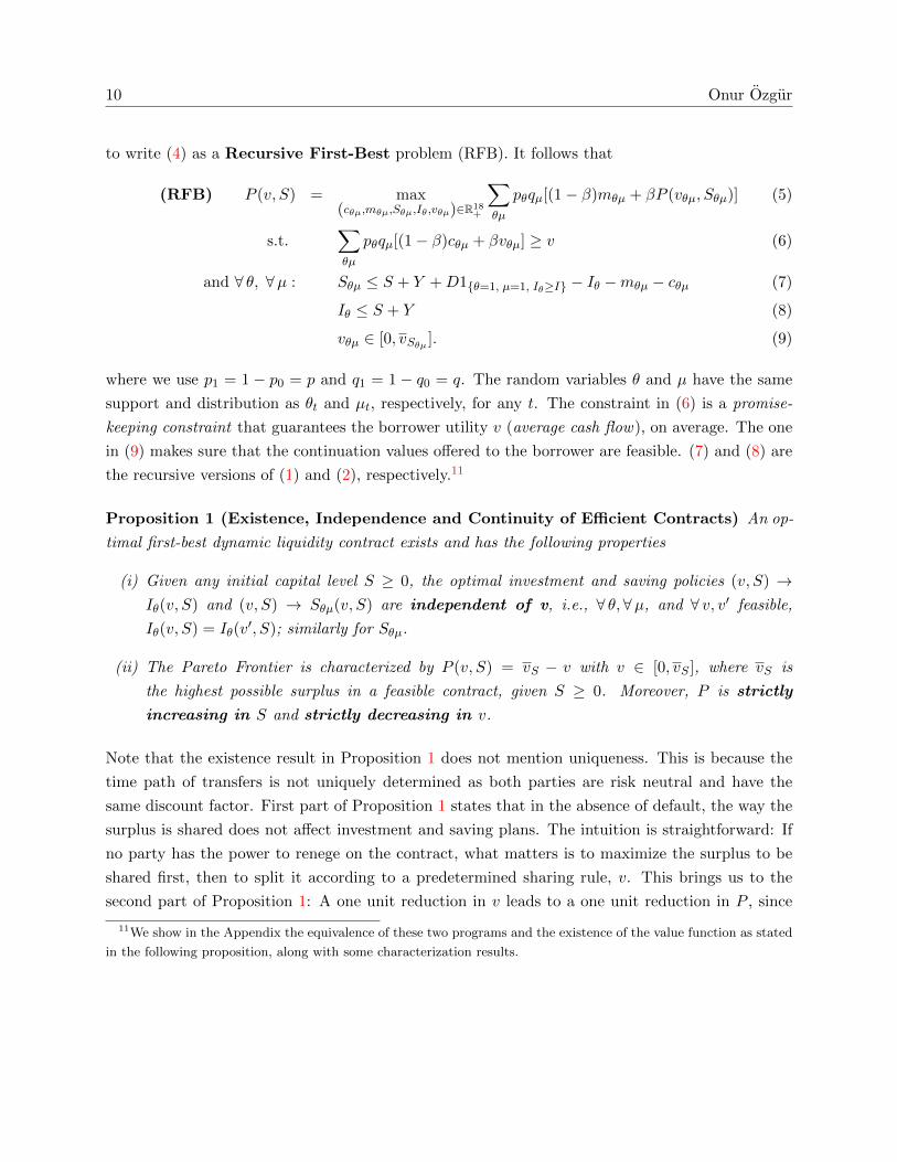
to write (4) as a Recursive First-Best problem (RFB). It follows that
(RFB) P (v, S) = max(cθµ,mθµ,Sθµ,Iθ,vθµ)∈R18
+
∑
θµ
pθqµ[(1− β)mθµ + βP (vθµ, Sθµ)] (5)
s.t.∑
θµ
pθqµ[(1− β)cθµ + βvθµ] ≥ v (6)
and ∀ θ, ∀µ : Sθµ ≤ S + Y +D1{θ=1, µ=1, Iθ≥I} − Iθ −mθµ − cθµ (7)
Iθ ≤ S + Y (8)
vθµ ∈ [0, vSθµ ]. (9)
where we use p1 = 1 − p0 = p and q1 = 1 − q0 = q. The random variables θ and µ have the same
support and distribution as θt and µt, respectively, for any t. The constraint in (6) is a promise-
keeping constraint that guarantees the borrower utility v (average cash flow), on average. The one
in (9) makes sure that the continuation values offered to the borrower are feasible. (7) and (8) are
the recursive versions of (1) and (2), respectively.11
Proposition 1 (Existence, Independence and Continuity of Efficient Contracts) An op-
timal first-best dynamic liquidity contract exists and has the following properties
(i) Given any initial capital level S ≥ 0, the optimal investment and saving policies (v, S) →Iθ(v, S) and (v, S) → Sθµ(v, S) are independent of v, i.e., ∀ θ,∀µ, and ∀ v, v′ feasible,
Iθ(v, S) = Iθ(v′, S); similarly for Sθµ.
(ii) The Pareto Frontier is characterized by P (v, S) = vS − v with v ∈ [0, vS ], where vS is
the highest possible surplus in a feasible contract, given S ≥ 0. Moreover, P is strictly
increasing in S and strictly decreasing in v.
Note that the existence result in Proposition 1 does not mention uniqueness. This is because the
time path of transfers is not uniquely determined as both parties are risk neutral and have the
same discount factor. First part of Proposition 1 states that in the absence of default, the way the
surplus is shared does not affect investment and saving plans. The intuition is straightforward: If
no party has the power to renege on the contract, what matters is to maximize the surplus to be
shared first, then to split it according to a predetermined sharing rule, v. This brings us to the
second part of Proposition 1: A one unit reduction in v leads to a one unit reduction in P , since
11We show in the Appendix the equivalence of these two programs and the existence of the value function as stated
in the following proposition, along with some characterization results.
Dynamic Liquidity Contracts 11
the optimal investment and saving policies are not affected from this change and that both agents
are risk neutral. We characterize next the recursive behavior of efficient saving and investment
policies.
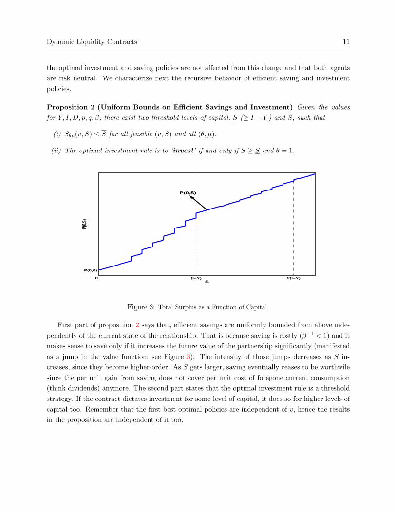
Proposition 2 (Uniform Bounds on Efficient Savings and Investment) Given the values
for Y, I,D, p, q, β, there exist two threshold levels of capital, S (≥ I − Y ) and S, such that
(i) Sθµ(v, S) ≤ S for all feasible (v, S) and all (θ, µ).
(ii) The optimal investment rule is to ‘invest’ if and only if S ≥ S and θ = 1.
0 (I−Y) 2(I−Y)
P(0,0)
Example of Value Function for Relatively Patient Agents
S
P(0,S
)
P(0,S)
Figure 3: Total Surplus as a Function of Capital
First part of proposition 2 says that, efficient savings are uniformly bounded from above inde-
pendently of the current state of the relationship. That is because saving is costly (β−1 < 1) and it
makes sense to save only if it increases the future value of the partnership significantly (manifested
as a jump in the value function; see Figure 3). The intensity of those jumps decreases as S in-
creases, since they become higher-order. As S gets larger, saving eventually ceases to be worthwile
since the per unit gain from saving does not cover per unit cost of foregone current consumption
(think dividends) anymore. The second part states that the optimal investment rule is a threshold
strategy. If the contract dictates investment for some level of capital, it does so for higher levels of
capital too. Remember that the first-best optimal policies are independent of v, hence the results
in the proposition are independent of it too.
12 Onur Ozgur
The next Proposition summarizes our initial idea of investment cycles generated by the liquidity
constraints on the lender. These are efficient cycles in the sense that they cannot be Pareto improved
upon by budget-balanced interventions.
Proposition 3 (Optimal Cycles) Given any economy, investment cycles are observed almost
surely, for economies with relatively patient agents. For low discount rates, the economy gets stuck in
a ‘credit crunch’ region with probability one, in finite time. Conditional on productive investment
being undertaken, the expected number of periods it takes the economy to move into a no-investment
state is an increasing function of the discount factor β and of the probability of productive investment
q.
The economic intuition is clear: for relatively patient parties, even if the joint capital level is
not sufficient to undertake positive NPV projects, the relationship does not collapse. The value
of the possibility of undertaking projects in the future is high enough to make the parties abide
by the contractual terms, build up capital to invest in the future. For relatively impatient parties,
that all works in the opposite direction. Once the economy gets into the ‘credit crunch’ region, it
stagnates there forever. There is no production in the economy anymore because the time value of
continuation by accumulating resources is too low compared to immediate consumption.
This result is important because the cycle argument does not necessitate any sort of agency
costs and/or inefficiency. These cycles are efficient cycles. There is no room for an authority to
intervene to improve upon the current allocation. We will see in section 4 that the likelihood of
these cycles increases with the introduction of agency costs due to the imperfect enforceability of
contracts.
3.1 Examples of Efficient Dynamics
The following will be our working example in this and the next section. The economy considered is
a special case of the general economy outlined above. Propositions 1 and 4 apply and I will give a
more explicit characterization of the optimal contract and use that to stress the important aspects
stemming from the incentive compatibility and the resource constraint. I first present the full
characterization of the first-best contracts for two classes of economies with relatively low discount
factors.
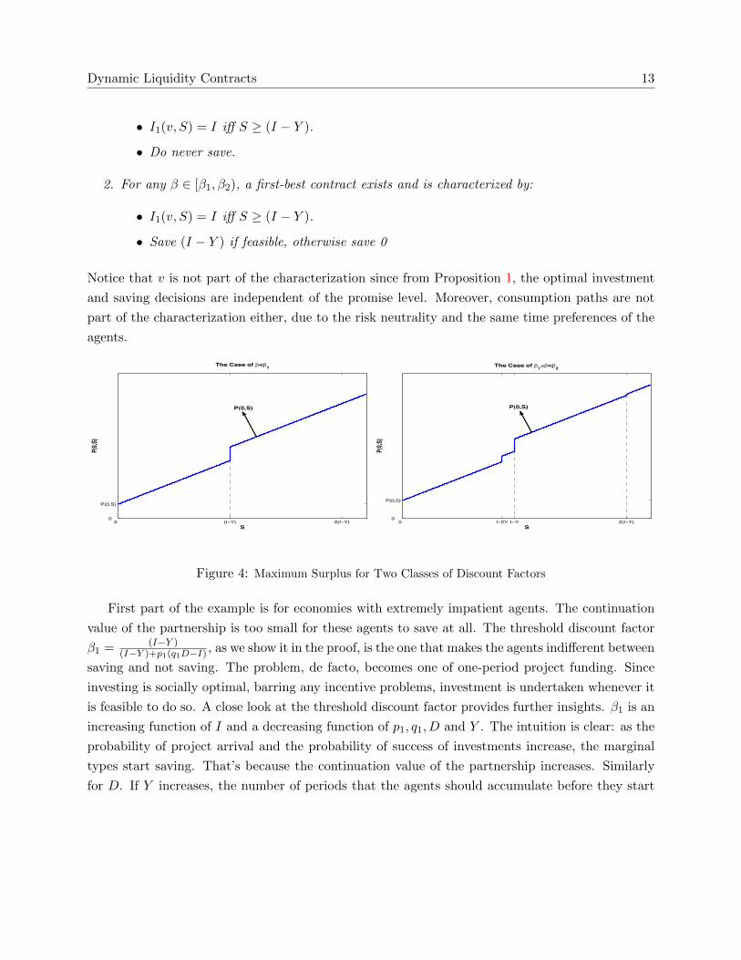
Example 1 Given the values for Y, I,D, p, q, there exist two threshold levels of the discount factor,
β1 and β2, where 0 < β1 < β2 < 1 such that the first-best contracts have the following properties
1. For any β ∈ [0, β1), a first-best contract exists and is characterized by:
Dynamic Liquidity Contracts 13
• I1(v, S) = I iff S ≥ (I − Y ).
• Do never save.
2. For any β ∈ [β1, β2), a first-best contract exists and is characterized by:
• I1(v, S) = I iff S ≥ (I − Y ).
• Save (I − Y ) if feasible, otherwise save 0
Notice that v is not part of the characterization since from Proposition 1, the optimal investment
and saving decisions are independent of the promise level. Moreover, consumption paths are not
part of the characterization either, due to the risk neutrality and the same time preferences of the
agents.
0 (I−Y) 2(I−Y)0
P(0,S)
The Case of !<!1
S
P(0,S
)
P(0,S)
0 I−2Y I−Y 2(I−Y)0
P(0,0)
The Case of !1"!<!2
S
P(0,S
)
P(0,S)
Figure 4: Maximum Surplus for Two Classes of Discount Factors
First part of the example is for economies with extremely impatient agents. The continuation
value of the partnership is too small for these agents to save at all. The threshold discount factor
β1 = (I−Y )(I−Y )+p1(q1D−I) , as we show it in the proof, is the one that makes the agents indifferent between
saving and not saving. The problem, de facto, becomes one of one-period project funding. Since
investing is socially optimal, barring any incentive problems, investment is undertaken whenever it
is feasible to do so. A close look at the threshold discount factor provides further insights. β1 is an
increasing function of I and a decreasing function of p1, q1, D and Y . The intuition is clear: as the
probability of project arrival and the probability of success of investments increase, the marginal
types start saving. That’s because the continuation value of the partnership increases. Similarly
for D. If Y increases, the number of periods that the agents should accumulate before they start

14 Onur Ozgur
investing decreases, which makes it worthwhile for some non-savers to start saving. A decrease in
the value of I works exactly in the same direction. Hence, the set of types (discount rates) who
will save becomes larger.
Second part is for agents who are “just patient” enough to save for the next period the amount
(I−Y ) that will make it feasible to invest in case of a productive shock. The added value of saving
more than this amount to self-insure for more than one period, is not enough to compensate for the
utility cost incurred. Similarly, it is not worth building the necessary stock to be able to invest in
case of a liquidity shock in the future, if the initial resources are too small. The same comparative
statics exercise that we did above for β1 can be undertaken for β2 and shown that β2 behaves the
same way.12
We now ask what happens in the two classes of economies in the longer run. For that purpose,
let the following be the set of states for the Markov aggregate system of our economy, generated
by the optimal investment and saving rules.
S ≡ {S∗ | S∗ is the optimal saving level for some level of end-of-period wealth}
Optimal savings are at the discontinuity points of the value function P . This is because saving
is relatively costly (or rate of return on deposits at the bank is smaller than the market interest
rate) and if savings are at a continuity point of P , there is always the temptation of cutting them
down since the gain from saving one unit less is (1−β) > β(1−β), the cost of continuing with one
unit less (P has constant slope (1 − β) at continuity points). Hence, in the case of the first class
of economies, S = {0}, since saving zero is the optimal strategy for any S. This is an ‘absorbing
state’ and the economy will be in that state forever at the period-ends, from second period on.
From the second period on, no investment projects will be undertaken. Capital will be depleted
and the economy will be in a constant state of stagnation.
For the second class of economies, the transitions are a bit more interesting. In this case,
S = {0, (I −Y )}. The Markov transition matrix, R, can be computed easily, by referring to Figure
2.
R ≡[
1 0
p1q0 1− p1q0
]
Let the first row denote state 0 and the second row represent state (I − Y ). For example, the
probability of moving from state (I − Y ) to state 0 is given by R21 = p1q0. The probability of
12Although we don’t have a clear explicit form for β2, a look at Figure 7 (in the Appendix) reveals that an increase
in p1, q1, D and Y pulls up the intersection of the function with the vertical axis, C, whereas a decrease in I takes the
function down by taking its value at β1 = −F , down. Both these movements make the intersection of the function
with the horizontal axis, β2, move to the left.
Dynamic Liquidity Contracts 15
ending up in the absorbing state in finite time is
1− limn→∞
(p1q0)n = 1
since it is simply the complement of the event ‘always in state (I − Y )’. Once again, the dynamics
are simple. From the second period on, if the capital level is sufficient to implement projects, the
economy stays in state (I−Y ), for some time, with positive probability. This is a very fragile state
since one bad shock (project failure) is sufficient to move the economy into the state of capital
crunch where it stays forever. The lender’s resource constraint binds; lender cannot provide the
borrower with any liquidity since he has no funds available. Positive net present value projects are
passed up. The interesting feature is that these are ‘efficient dynamics’.
4 Optimal Dynamic Liquidity Contracts with Strategic Default
In this section, I study equilibrium contracts when the borrower can no longer commit. He has
the opportunity to renege on the agreement after the investment is undertaken and can run away
with the return on investment that he confiscates. Remember that the borrower is excluded from
the credit markets forever in case he defaults. The lender commits to the terms of the contract
as long as his participation constraint is satisfied at t = 0. A second-best liquidity contract, then,
analogously to the first-best, is said to be feasible if it is an element of the following set with initial
capital level S,13
Definition 3 Let ΣSB(S) ={σ = (ct,mt, It, St+1) that satisfy (1)-(3), with S0 = S and an in-
centive compatibility constraint (IC), i.e., ∀t, ∀ht,
(1− β) ct(ht) + β EUB(σ | ht) ≥ (1− β)D 1{θt=1, µt=1 and It(ht−1,θt)≥I} + β Y
Taking these constraints into account, second-best contracts will be the solutions to the following
program
Q(v, S) = maxσ∈ΣSB(S)
{EUL(σ) | EUB(σ) ≥ v
}(10)
where v is feasible in the sense that there exists a feasible contract σ that yields the borrower at
least v ex-ante. Notice that the above constraints are “best deviation” constraints for the borrower.13Alternatively, one can divide the joint capital level S into SL and SB and track them separately. This complicates
the computations and the presentation with no apparent contribution to economic insight. In such a treatment, the
borrower would keep SB with the bank since he has no other way of storing and the bank can confiscate SB in case
the borrower defaults. This division argument might yield different results in the presence of competing multiple
lenders and access to credit markets, which are outside the scope of the current paper.

16 Onur Ozgur
In general, the borrower might deviate from what the allocation prescribes in many different ways;
none of these yields him a higher payoff then does the best deviation strategy. Thus, if a contract
satisfies the best deviation constraints, it will be incentive compatible.
The program above can be written recursively, using v and S as state variables. These two
are “sufficient statistics” providing the necessary information required to solve for the second-best
contract. Hence, the recursive second-best program (RSB) is
(RSB) Q(v, S) = max(cθµ,mθµ,Sθµ,Iθ,vθµ)∈R18
+
∑
θµ
pθqµ[(1− β)mθµ + βQ(vθµ, Sθµ)]
s.t.∑
θµ
pθqµ[(1− β)cθµ + βvθµ] ≥ v (11)
Sθµ ≤ S + Y +D 1{θ=1, µ=1, Iθ≥I} − Iθ −mθµ − cθµ (12)
Iθ ≤ S + Y (13)
(1− β) cθµ + βvθµ ≥ (1− β)D 1{θ=1, µ=1, Iθ≥I} + β Y (14)
vθµ ∈ [Y, vSθµ ]. (15)
The extra constraint (14) guarantees that the borrower gets a utility level at least as high as
what he gets by defaulting, on the paths where investment is undertaken and it succeeds. On other
paths, (14) is implied by (15). The next result is at the core of our analysis. It fully characterizes
optimal liquidity contracts while at the same time making sure that at least one exists.
Proposition 4 (i) An optimal second-best contract exists.
(ii) There exists an S ≥ (I−Y ) such that for all S ≥ S, there are two promise values 0 ≤ v∗(S) ≤v∗(S) ≤ vS with
(a) I1(v, S) = 0, for v ∈ [Y, v∗(S)],
(b) I1(v, S) = I, for v ∈ [v∗(S), vS ]
(c) The value function in (RSB) is given by
Q(v, S) =
vS − v if v ≥ v∗(S)
vS − v∗(S) if v ∈ [v∗(S), v∗(S)]
vS − [v∗(S)− v∗(S)]− v if v ∈ [Y, v∗(S)]
(d) v∗(S) is nondecreasing in S.
Dynamic Liquidity Contracts 17
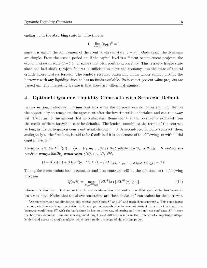
The statements in Proposition 4, which are also depicted in Figure 5, carry a nice economic
intuition. For each level of v and S, the number of ways the incentives can affect the first-best
utility levels is two. What distinguishes the graph on the left from the one on the right is the fact
that, first-best optimal policies are also second-best optimal on the left. On the right, below a level
of v, investment is not undertaken under the second-best rule although it is under the first-best rule.
Notice that, both these cases refer to the first-best optimal ‘Invest’ regime. When the first-best
rule is not to invest in the current period, there is no distributional conflicts arising from incentive
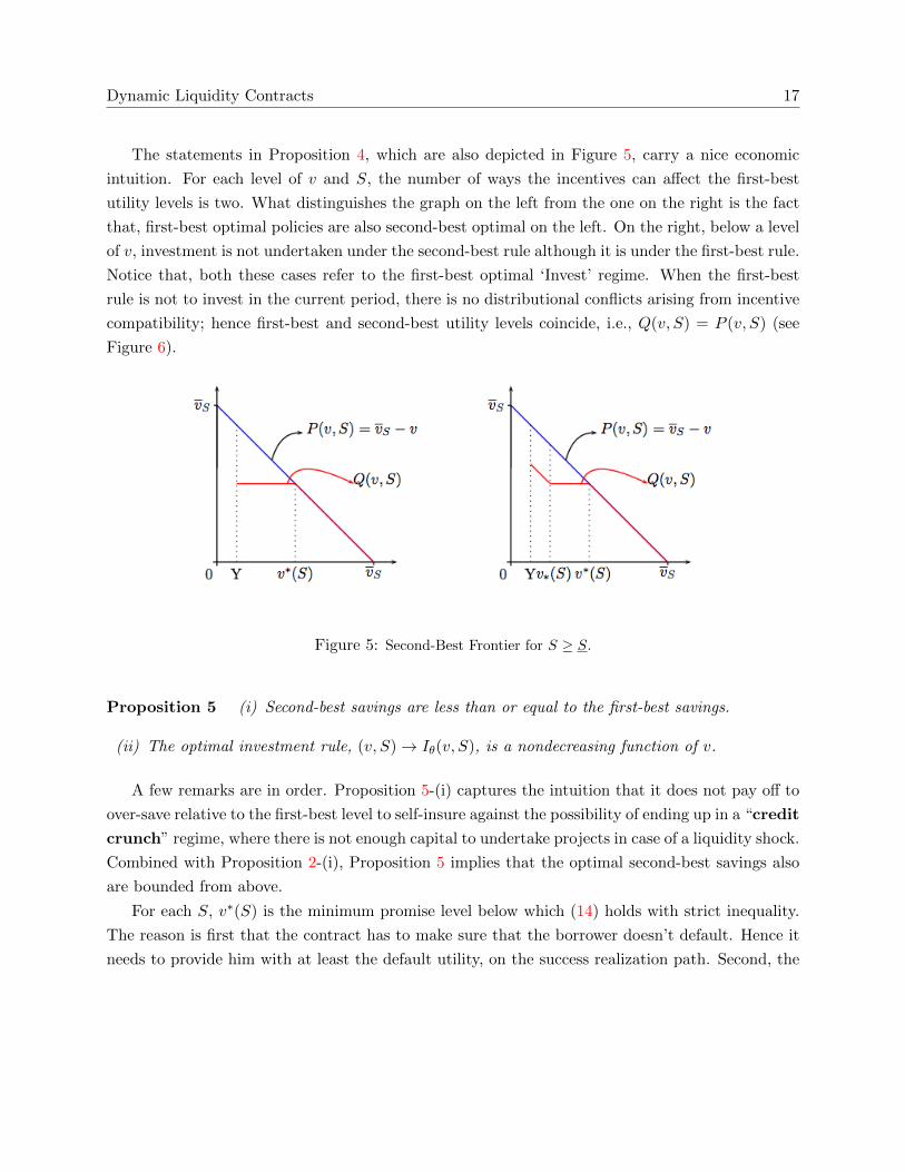
compatibility; hence first-best and second-best utility levels coincide, i.e., Q(v, S) = P (v, S) (see
Figure 6).
Figure 5: Second-Best Frontier for S ≥ S.
Proposition 5 (i) Second-best savings are less than or equal to the first-best savings.
(ii) The optimal investment rule, (v, S)→ Iθ(v, S), is a nondecreasing function of v.
A few remarks are in order. Proposition 5-(i) captures the intuition that it does not pay off to
over-save relative to the first-best level to self-insure against the possibility of ending up in a “credit
crunch” regime, where there is not enough capital to undertake projects in case of a liquidity shock.
Combined with Proposition 2-(i), Proposition 5 implies that the optimal second-best savings also
are bounded from above.
For each S, v∗(S) is the minimum promise level below which (14) holds with strict inequality.
The reason is first that the contract has to make sure that the borrower doesn’t default. Hence it
needs to provide him with at least the default utility, on the success realization path. Second, the
18 Onur Ozgur
Figure 6: Second-Best Frontier for S < S.
continuation promise levels must satisfy the borrower’s individual rationality constraint. Hence,
even if the initial level of v is below v∗(S), the de facto payment, on average is equal to v∗(S).
For some parameterizations, there is another threshold level v∗(S) below which “rationing the
credit” is optimal although it is socially optimal to undertake the investment in the absence of
incentive problems. The idea is that, if investment is undertaken, the cost of making sure that
the borrower does not default is so high that the lender prefers not extending the credit although
first-best requires him to do so.
The fact that first-best and second-best investment and saving decisions might not agree lead
to the following important conclusion: investment cycles might become further skewed toward states
of liquidity drought. The reason is straightforward. The only reason agents save in this economy
is to make sure that productive investment opportunities do not go unimplemented. The lack of
enforcement diminishes the future value of the partnership hence making it less appealing to save
for the future. Consequently, it becomes more likely that the system ends up in the ‘liquidity
drought’ region. In a similar fashion, low collateral (proxied by v) on the part of the borrower
can make it extremely costly to keep the borrower from reneging, which in turn leads to credit
being rationed; this is another channel through which the flow of new capital into the system is
interrupted which in turn makes the possibility of liquidity drought more likely.
As we did for the first-best contracts, we now turn to two classes of economies where we can
solve for the contracts in closed form and shed light on the second-best dynamics.
Dynamic Liquidity Contracts 19
4.1 Second-Best Dynamics
Here, we take it from where we left in the previous section’s Example 1 and analyze the behavior
of the second-best contracts and compare it to the benchmark case of first-best contracts. The
explicit characterization of the former for both economies makes it clear what kind of distortions
the enforceability problems cause to the socially optimal allocations and utility levels.
Example 2 1. For any β ∈ (0, β1), a stationary second-best contract exists and is characterized
by:
(a) For S ≥ I − Y , there exist 0 ≤ v∗(S) ≤ v∗(S) ≤ vS such that
i. I1(v, S) = 0, for v ∈ [Y, v∗(S)],
ii. I1(v, S) = I, for v ∈ [v∗(S), vS ]
(b) Do never save
(c) We have the figure on the right iff p1 >YI .
2. For any β ∈ [β1, β2), a stationary second-best contract exists and is characterized by:
(a) For S ≥ I − Y , there exist 0 ≤ v∗(S) ≤ v∗(S) ≤ vS such that
i. I1(v, S) = 0, for v ∈ [Y, v∗(S)],
ii. I1(v, S) = I, for v ∈ [v∗(S), vS ]
(b) Save (I − Y ) if feasible, otherwise save 0
One interesting feature of the first class of economies is the fact that we have the second-best
frontier on the right hand side of Figure 5 if p1 >YI . So, if the probability of a liquidity shock is too
high, the lender does not extend credit to borrowers with little colateral, v ∈ [Y, v∗(S)), because
it is too costly to ensure no-default in case investment is undertaken; an increase in p1 raises the
weight of that state in the expected utility computation.
5 Conclusion
In this paper, I studied the nature of long-term liquidity provision between lenders and borrowers
in the absence of perfect enforceability and when both parties are financially constrained. To this
end, I built a tractable infinite horizon model of long-term lending and borrowing and analyzed in
what ways liquidity shortages on both parties affect the evolution of the economy and investment
activity in particular.

20 Onur Ozgur
I show that enforcement problems and endogenous resource constraints can severely reduce the
possibility of financing projects. Investment and saving decisions depend not only on the level of
capital but also on the surplus sharing rule, in contrast to the first-best contracts. Investment is
(weakly) under-provided. Second-best savings are (weakly) less than first-best savings capturing
the intuition that it does not pay off to postpone consumption/investment to self-insure against a
possible ‘credit crunch’.
I also show that the economy exhibits investment cycles of two different natures. First type
of cycles happen because the lenders are credit constrained; these are efficient cycles. The second
type of cycles are due to incentive compatibility. The punchline is: credit is rationed if either the
lender has too little capital or the borrower has too little financial collateral.
The present work’s technical contribution is to show the existence and characterization of fi-
nancial contracts that are solutions to a non-convex dynamic programming problem.
As in any model, I left out many things. The first next step in this research program should
be to build and analyze a model in which the opportunity cost (capital constraint) of lenders
is endogenized by studying explicitly the credit markets as a dynamic game between lenders for
loanable funds. The introduction of competition among lenders would not only enrich the story
that I am telling, but also would make it possible to think in a realistic way about renegotiation
issues, reputation building on the part of the lender/borrower, and endogenous opportunity costs
and credit rationing due to locking-up with a current set of borrowers (or lenders).
There is a couple of other points that are of importance for future research: One should look
at economies where there are both aggregate and micro level liquidity shocks and consider het-
erogeneity among lenders and borrowers. Heterogeneity and aggregate uncertainty introduces the
possibility of intra-institutional arrangements in a dynamic setting, that the present model cannot
capture. Of course, all of this is for future work.
6 Appendix
Proof of Proposition 1
Period utility functions and the space of feasible resources are unbounded. I first show that at the
optimum, the set{EUL(σ) | EUB(σ) ≥ v, σ ∈ ΣFB(S)
}is bounded from above by the value of a
relaxed program for which the supremum exists and is finite-valued. This latter defines a set, F , of
feasible (v, S) pairs. I define a functional space, B(F ) and an operator, T , on that functional space,
which is associated with the (RFB) problem in (5). The ‘limited liability’ assumption implies that

Dynamic Liquidity Contracts 21
the value function be non-negative for any feasible value of v in the first-best program. So, the
value function itself enters the constraint set of the problem. This brings up the question ‘what is
the set of feasible values of v’ for any given S. I will first prove a series of 3 Lemmas which, put
together, will deliver the results of interest.
Let P ∗(v, S) be the value of the supremum in the first-best problem in (4) parameterized by
S0 = S ≥ 0 and a feasible v. I first show that the supremum of the sequence problem exists and
is attained by a contract. Then, I proceed to show that the unique fixed point of the operator T ,
associated with the (RFB) problem, defined on the ‘right’ space of candidate value functions, is
actually P ∗. Finally, I characterize the first-best frontier and first-best contracts.
Lemma 1 P ∗(v, S) exists and is attained by an optimal contract such that P ∗(v, S) ≤ (1− β)S +Y + p1q1(D − I). In particular, (1− β)S + Y ≤ P ∗(0, S) ≤ (1− β)S + Y + p1q1(D − I).
Proof: The following program is a relaxed version of the first-best problem in (4) with v = 0,
where the economy generates Y with certainty and (D − I) extra with probability p1q1, every
period.
sup(mt,St+1)∞t=0
E(1− β)
∞∑
t=0
βtmt
s.t. ∀t, ∀ht St+1(ht) ≤ St(ht−1)−mt(ht) + Y + (D − I)1{θt=1, µt=1} (16)
mt, St+1 ≥ 0 and S0 = S ≥ 0 is given.
The objective is linear and the constraint set is convex. So, this is a concave programming problem.
Hence, the first-order conditions are necessary and sufficient for a maximum. Partially differenti-
ating the objective with respect to St+1(ht) gives
−Prob(ht)βt(1− β) + Prob(ht)βt+1(1− β) < 0
which implies that St+1(ht) = 0 for all ht. Hence, the agent consumes all his wealth at the end of
each period. The supremum is achieved and by simple algebra, is equal to
(1− β)S + Y + p1q1(D − I)
Clearly, any contract that is feasible for the original problem is also feasible for the relaxed problem.
Consequently, the supremum of the original problem exists and P ∗(0, S) ≤ (1−β)S+Y +p1q1(D−I).
Since the constraint set of the problem with v 6= 0 is smaller than that of the problem with v = 0,
we also have P ∗(v, S) ≤ P ∗(0, S) for any (v, S) feasible. Supremum in (16) is attained by an

22 Onur Ozgur
optimal contract because the constraint set defined by a sequence of weak inequalities is closed.
Hence, the sup operator in the statement of the problem can be replaced by a max operator and an
optimal contract can be computed for each S and v. One feasible strategy in the original problem
is to ‘never invest ’ after any history. Conditioning on ‘never investing’, the optimal strategy solves
max(mt,St+1)∞t=0
E(1− β)∞∑
t=0
βtmt
s.t. ∀t, ∀ht St+1(ht) ≤ St(ht−1)−mt(ht) + Y
mt, St+1 ≥ 0 and S0 = S ≥ 0 is given.
By the same token as above, the maximum is achieved and is equal to (1 − β)S + Y . Since this
is a possibly suboptimal strategy, we have (1 − β)S + Y ≤ P ∗(0, S). Gathering both sides of the
inequalities together, we obtain the stated result. Q.E.D.
Let F be the set of (v, S) pairs for which a feasible contract exists; namely
F ≡{
(v, S) ∈ R2+ | v ≤ P ∗(0, S)
}
Naturally, the ‘right’ space for our problem is the space of non-negative valued functions on F , that
are non-increasing in v, non-decreasing in S and bounded above by the function (1 − β)S + Y +
p1q1(D − I). Namely,
B(F ) := {f : F → R+ | s.t. (i)− (iii) hold where}(i) f(v′, S) ≤ f(v, S) for v′ > v
(ii) f(v, S) ≤ f(v, S′) for S′ > S
(iii) 0 ≤ f(v, S) ≤ (1− β)S + Y + p1q1(D − I)
Let T be an operator defined on B(F ) such that, for any (v, S) ∈ F and any P ∈ B(F ):
(TP )(v, S) = max(cθµ,mθµ,Sθµ,Iθ,vθµ)∈R18
+
∑
θµ
pθqµ[(1− β)mθµ + βP (vθµ, Sθµ)]
s.t. ∀θ, ∀µ (vθµ, Sθµ) ∈ F (17)
Sθµ ≤ S + Y +D1{θ=1, µ=1, Iθ≥I} − Iθ −mθµ − cθµIθ ≤ S + Y∑
θµ
pθqµ[(1− β)cθµ + βvθµ] ≥ v

Dynamic Liquidity Contracts 23
Lemma 2 T : B(F )→ B(F ) and P ∗ is its unique fixed point.
Proof: (TP )(v, S) ≥ 0 for any (v, S) ∈ F and P ∈ B(F ) due to limited liability and the non-
negativity of P . Let P (v, S) ≡ (1−β)S+Y +p1q1(D−I) be the upper bound function for elements
of B(F ). P clearly is an element of B(F ). With P being the continuation function, the optimal
consumption/saving decision is to consume everything at the end of the period. Conditioning on
that, the optimal investment strategy is to invest whenever it is feasible. But then,
(TP )(v, S) ≤ (TP )(0, S) =
{(1− β)S + Y + p1q1D − (1− βq0)p1I, if S ≥ I − Y(1− β)S + Y + βp1q1(D − I), if S < I − Y.
≤ P (v, S)
Clearly, T is monotonic in P and (TP ) is non-increasing in v and nondecreasing in S which makes
the latter an element of B(F ). Hence, 0 ≤ (TP )(v, S) ≤ (TP )(v, S) ≤ P (v, S) for any (v, S) ∈ Fand P ∈ B(F ). This establishes that T is a self-map.
P ∗ ∈ B(F ) and by standard arguments (see Stokey and Lucas (1989), Theorem 4.2), TP ∗ = P ∗.
The next step is to show that this is the only fixed point of the operator T . What is required is a
boundedness condition, limn→∞
βnP (vn, Sn) = 0, where (vn, Sn)∞n=0 is a particular realization path of
a feasible contract from (S0, v0). This condition requires the value function to be bounded on any
realized path from (v0, S0) for a feasible contract, and is sufficient to guarantee that any P that
satisfies this condition is actually the supremum function. We will show that limn→∞
βnP (vn, Sn) = 0
for any fixed point P of T . Since there is a finite number of states of nature each period, Theorem
4.3 in Stokey and Lucas (1989) can be modified to argue that any fixed point P of (17) that satisfies
the boundedness condition is actually the supremum function P ∗.
The fastest accumulation path for the problem in (16) is S1 = S0 + Y + p1q1(D − I), S2 =
S1 + Y + p1q1(D− I) = S0 + 2(Y + p1q1(D− I)), . . . , Sn = S0 +n(Y + p1q1(D− I)), . . . Clearly, it
is so for the original problem, too. Hence for any realized feasible path (v∗n, S∗n)∞n=0 of the original
problem, we have
P (v∗n, S∗n) ≤ P (0, S∗n) ≤ P (v∗n, Sn)
The discounted versions respect the same ordering
βnP (v∗n, S∗n) ≤ βnP (0, S∗n) ≤ βnP (v∗n, Sn)
Substituting for P (v∗n, Sn), we have
βnP (v∗n, Sn) = βn [(1− β)(S0 + n(Y + p1q1(D − I)) + Y + p1q1(D − I)]

24 Onur Ozgur
which goes to zero as n goes to infinity. Therefore, so does βnP (v∗n, S∗n). By the argument in the
previous paragraph, P = P ∗. Q.E.D.
Let P be the supremum function which is also the unique fixed point of (17) by Lemma 2.
Then, P (0, S) is the maximum possible surplus with initial capital level S, due to the following
Lemma.
Lemma 3 The optimal investment and saving strategies (It, St+1)∞t=0 depend only on S, not on v.Moreover, P (v, S) = P (0, S)− v for v ∈ [0, P (0, S)].
Proof: Let (m∗t , I∗t , S
∗t+1)∞t=0 be the optimal contract that achieves the supremum in the first-
best with v = 0 and S0 = S. Let v ∈ [0, P (0, S)]. We will first construct (c∗∗t ,m∗∗t , I
∗∗t , S
∗∗t+1)∞t=0
where c∗∗t = αm∗t and m∗∗t = (1− α)m∗t , where α ∈ (0, 1) is s.t.
v = E(1− β)∞∑
t=0
βtc∗∗t = αE(1− β)∞∑
t=0
βtm∗t
and S∗∗t+1 = S∗t+1, I∗∗t = I∗t as before. Clearly, this new contract is feasible and achieves the
utility level v for the borrower. Now, suppose for a contradiction that the new contract is Pareto
dominated by (c′t,m′t, I′t, S′t+1)∞t=0, the new optimizer. Therefore,
v = E(1− β)
∞∑
t=0
βtc′t
since the IR constraint for the borrower binds necessarily at the optimum
P (v, S) = E(1− β)
∞∑
t=0
βtm′t > E(1− β)
∞∑
t=0
βtm∗∗t = E(1− β)
∞∑
t=0
βtm∗t (1− α)
But this is going to imply that the original contract for v = 0 could not have been optimal. Let’s
define the contract (c′′t ,m′′t , I′′t , S
′′t+1)∞t=0 by c′′t (h
t) = 0, m′′t (ht) = (m′t(h
t) + c′t(ht)) with I ′′t = I ′t and
S′′t+1 = S′t+1. This is clearly feasible for the problem with v = 0 and
P (0, S) ≥ E(1− β)∞∑
t=0
βtm′′t = E(1− β)∞∑
t=0
βt(c′t +m′t)
> E(1− β)
∞∑
t=0
βtc′t + E(1− β)
∞∑
t=0
βtm∗t (1− α)
= αP (0, S) + (1− α)P (0, S)
= P (0, S)

Dynamic Liquidity Contracts 25
a contradiction. As to the second claim, the contract (c∗∗t ,m∗∗t , I
∗∗t , S
∗∗t+1)∞t=0 is shown to be feasible
and achieve the supremum for the first-best program with v ∈ (0, P (0, S)). Hence,
P (v, S) = E(1− β)∞∑
t=0
βtm∗∗t
= E(1− β)
∞∑
t=0
βt(1− α)m∗t
= (1− α)E(1− β)∞∑
t=0
βtm∗t
= P (0, S)− v
from the definition of α. Q.E.D.
Lemmas (1)-(3) put together prove Proposition 1.
Q.E.D.
Proof of Proposition 2
Part (i): Suppose for a contradiction that for any S, there is an S′ such that for some (v, S) and
(θ, µ), S′ = Sθµ(v, S) > S. Then, we can construct a nondecreasing sequence (S′n):
S′n = Sθnµn(vn, Sn) > n , for n ∈ N
for some (vn, Sn) feasible, and (θn, µn) for each n. Let Wn be the end-of-period wealth on the
realized path corresponding to (vn, Sn) and (θn, µn). Clearly, this sequence is unbounded and for
each consecutive terms, we have (since first-best decisions are independent of v due to Proposition
1)
(1− β)[Wn+1 − S′n] + βP (0, S′n) ≤ (1− β)[Wn+1 − S′n+1] + βP (0, S′n+1)
due to optimality, with at least one strict inequality. But, then this ordering is independent of the
particular wealth level since we can just get rid of those from both sides of the inequality. Hence,
(1− β)[−S1] + βP (0, S1) < (1− β)[−Sn+1] + βP (0, Sn+1)
for large n. This in turn implies that
P (0, Sn+1)− P (0, S1)
Sn+1 − S1>
(1− β)
β> (1− β)
26 Onur Ozgur
Hence, P should increase, on average, with a slope larger than (1 − β)/β, greater than (1 − β).
This would imply that P should intersect the line (1 − β)S + Y + p1q1(D − I) eventually, which
is a contradiction since that is an upper bound for P from Lemma 1. Moreover, this level S is
achieved by the same token above. For large levels of W , S and everything less than that will be
available. Since P is bounded above and P is clearly right-continuous, there is a threshold level of
end-of-period wealth after which optimal savings are S.
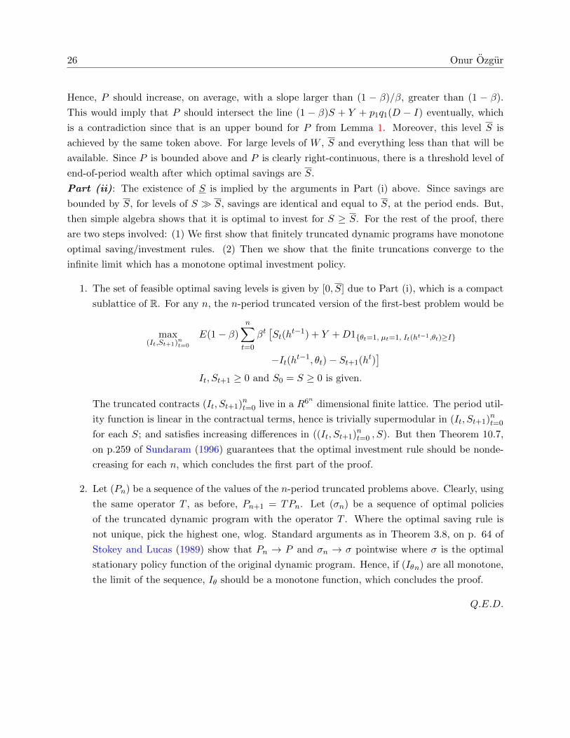
Part (ii): The existence of S is implied by the arguments in Part (i) above. Since savings are
bounded by S, for levels of S � S, savings are identical and equal to S, at the period ends. But,
then simple algebra shows that it is optimal to invest for S ≥ S. For the rest of the proof, there
are two steps involved: (1) We first show that finitely truncated dynamic programs have monotone
optimal saving/investment rules. (2) Then we show that the finite truncations converge to the
infinite limit which has a monotone optimal investment policy.
1. The set of feasible optimal saving levels is given by [0, S] due to Part (i), which is a compact
sublattice of R. For any n, the n-period truncated version of the first-best problem would be
max(It,St+1)nt=0
E(1− β)n∑
t=0
βt[St(h
t−1) + Y +D1{θt=1, µt=1, It(ht−1,θt)≥I}
−It(ht−1, θt)− St+1(ht)]
It, St+1 ≥ 0 and S0 = S ≥ 0 is given.
The truncated contracts (It, St+1)nt=0 live in a R6n dimensional finite lattice. The period util-
ity function is linear in the contractual terms, hence is trivially supermodular in (It, St+1)nt=0
for each S; and satisfies increasing differences in ((It, St+1)nt=0 , S). But then Theorem 10.7,
on p.259 of Sundaram (1996) guarantees that the optimal investment rule should be nonde-
creasing for each n, which concludes the first part of the proof.
2. Let (Pn) be a sequence of the values of the n-period truncated problems above. Clearly, using
the same operator T , as before, Pn+1 = TPn. Let (σn) be a sequence of optimal policies
of the truncated dynamic program with the operator T . Where the optimal saving rule is
not unique, pick the highest one, wlog. Standard arguments as in Theorem 3.8, on p. 64 of
Stokey and Lucas (1989) show that Pn → P and σn → σ pointwise where σ is the optimal
stationary policy function of the original dynamic program. Hence, if (Iθn) are all monotone,
the limit of the sequence, Iθ should be a monotone function, which concludes the proof.
Q.E.D.
Dynamic Liquidity Contracts 27
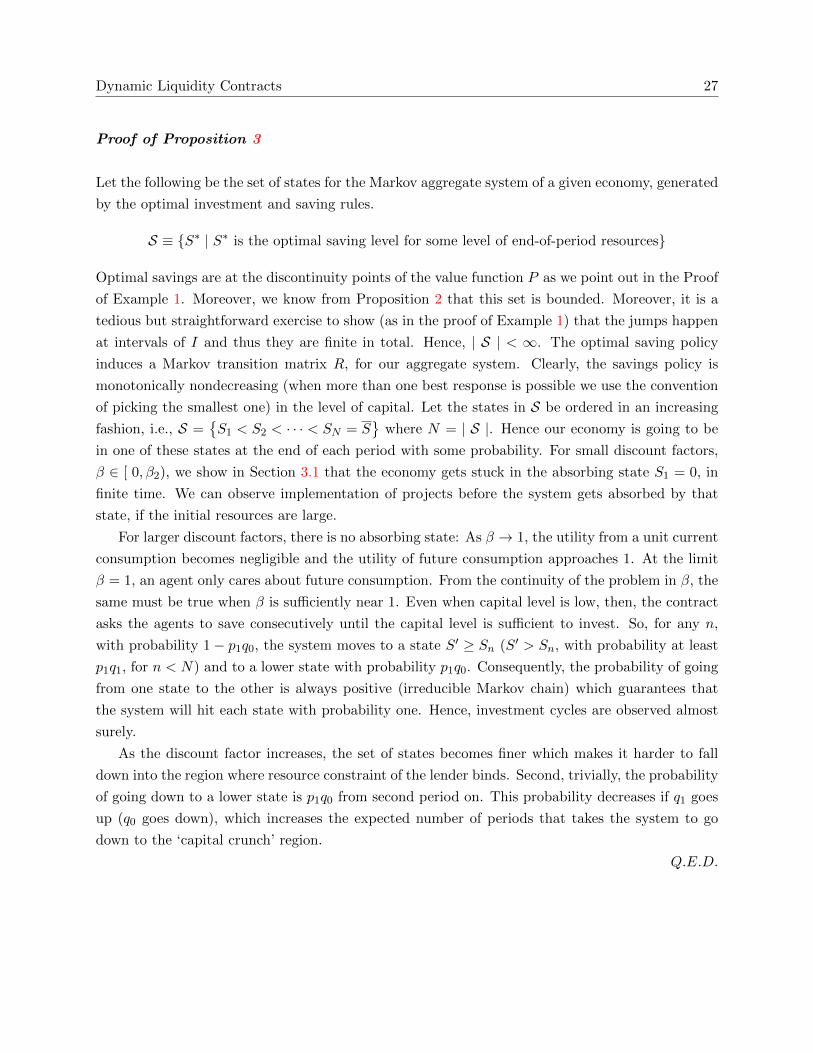
Proof of Proposition 3
Let the following be the set of states for the Markov aggregate system of a given economy, generated
by the optimal investment and saving rules.
S ≡ {S∗ | S∗ is the optimal saving level for some level of end-of-period resources}
Optimal savings are at the discontinuity points of the value function P as we point out in the Proof
of Example 1. Moreover, we know from Proposition 2 that this set is bounded. Moreover, it is a
tedious but straightforward exercise to show (as in the proof of Example 1) that the jumps happen
at intervals of I and thus they are finite in total. Hence, | S | < ∞. The optimal saving policy
induces a Markov transition matrix R, for our aggregate system. Clearly, the savings policy is
monotonically nondecreasing (when more than one best response is possible we use the convention
of picking the smallest one) in the level of capital. Let the states in S be ordered in an increasing
fashion, i.e., S ={S1 < S2 < · · · < SN = S
}where N = | S |. Hence our economy is going to be
in one of these states at the end of each period with some probability. For small discount factors,
β ∈ [ 0, β2), we show in Section 3.1 that the economy gets stuck in the absorbing state S1 = 0, in
finite time. We can observe implementation of projects before the system gets absorbed by that
state, if the initial resources are large.
For larger discount factors, there is no absorbing state: As β → 1, the utility from a unit current
consumption becomes negligible and the utility of future consumption approaches 1. At the limit
β = 1, an agent only cares about future consumption. From the continuity of the problem in β, the
same must be true when β is sufficiently near 1. Even when capital level is low, then, the contract
asks the agents to save consecutively until the capital level is sufficient to invest. So, for any n,
with probability 1− p1q0, the system moves to a state S′ ≥ Sn (S′ > Sn, with probability at least
p1q1, for n < N) and to a lower state with probability p1q0. Consequently, the probability of going
from one state to the other is always positive (irreducible Markov chain) which guarantees that
the system will hit each state with probability one. Hence, investment cycles are observed almost
surely.
As the discount factor increases, the set of states becomes finer which makes it harder to fall
down into the region where resource constraint of the lender binds. Second, trivially, the probability
of going down to a lower state is p1q0 from second period on. This probability decreases if q1 goes
up (q0 goes down), which increases the expected number of periods that takes the system to go
down to the ‘capital crunch’ region.
Q.E.D.
28 Onur Ozgur
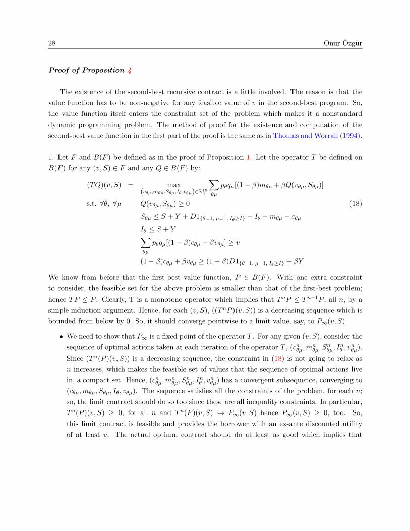
Proof of Proposition 4
The existence of the second-best recursive contract is a little involved. The reason is that the
value function has to be non-negative for any feasible value of v in the second-best program. So,
the value function itself enters the constraint set of the problem which makes it a nonstandard
dynamic programming problem. The method of proof for the existence and computation of the
second-best value function in the first part of the proof is the same as in Thomas and Worrall (1994).
1. Let F and B(F ) be defined as in the proof of Proposition 1. Let the operator T be defined on
B(F ) for any (v, S) ∈ F and any Q ∈ B(F ) by:
(TQ)(v, S) = max(cθµ,mθµ,Sθµ,Iθ,vθµ)∈R18
+
∑
θµ
pθqµ[(1− β)mθµ + βQ(vθµ, Sθµ)]
s.t. ∀θ, ∀µ Q(vθµ, Sθµ) ≥ 0 (18)
Sθµ ≤ S + Y +D1{θ=1, µ=1, Iθ≥I} − Iθ −mθµ − cθµIθ ≤ S + Y∑
θµ
pθqµ[(1− β)cθµ + βvθµ] ≥ v
(1− β)cθµ + βvθµ ≥ (1− β)D1{θ=1, µ=1, Iθ≥I} + βY
We know from before that the first-best value function, P ∈ B(F ). With one extra constraint
to consider, the feasible set for the above problem is smaller than that of the first-best problem;
hence TP ≤ P . Clearly, T is a monotone operator which implies that TnP ≤ Tn−1P , all n, by a
simple induction argument. Hence, for each (v, S), ((TnP )(v, S)) is a decreasing sequence which is
bounded from below by 0. So, it should converge pointwise to a limit value, say, to P∞(v, S).
• We need to show that P∞ is a fixed point of the operator T . For any given (v, S), consider the
sequence of optimal actions taken at each iteration of the operator T , (cnθµ,mnθµ, S
nθµ, I
nθ , v
nθµ).
Since (Tn(P )(v, S)) is a decreasing sequence, the constraint in (18) is not going to relax as
n increases, which makes the feasible set of values that the sequence of optimal actions live
in, a compact set. Hence, (cnθµ,mnθµ, S
nθµ, I
nθ , v
nθµ) has a convergent subsequence, converging to
(cθµ,mθµ, Sθµ, Iθ, vθµ). The sequence satisfies all the constraints of the problem, for each n;
so, the limit contract should do so too since these are all inequality constraints. In particular,
Tn(P )(v, S) ≥ 0, for all n and Tn(P )(v, S) → P∞(v, S) hence P∞(v, S) ≥ 0, too. So,
this limit contract is feasible and provides the borrower with an ex-ante discounted utility
of at least v. The actual optimal contract should do at least as good which implies that

Dynamic Liquidity Contracts 29
(TP∞)(v, S) ≥ P∞(v, S). We also know, from the monotonicity of the operator T , that, for all
n, (TnP )(v, S) ≤ (Tn−1P )(v, S) hence (Tn−1P )(v, S) ≥ P∞(v, S). Therefore, (TnP )(v, S) ≥(TP∞)(v, S) for all n which implies that the limit of that sequence admits the same ordering:
(TnP )(v, S) → P∞(v, S) ≥ (TP∞)(v, S). We showed that P∞(v, S) ≥ (TP∞)(v, S) and
P∞(v, S) ≤ (TP∞)(v, S) which implies that P∞(v, S) = (TP∞)(v, S) hence P∞ is a fixed
point of the operator T .
• Clearly, each fixed point Q of the operator T corresponds to a second-best contract. It is
the standard unravelling idea. Start with an initial (v, S); the optimal actions in period 1
are given by (cθµ,mθµ, Sθµ, Iθ, vθµ). Let σ1 be defined as c1(θ, µ) = cθµ, m1(θ, µ) = mθµ,
S2(θ, µ) = Sθµ and I1(θ) = Iθ. The second period contract conditional on the realization of
θ, µ in the first period is the optimal action vector starting with an initial (vθµ, S2(θ, µ)), and
so on by repeatedly applying the operator T . The contract σ constructed this way satisfies all
the constraints of the original second-best problem and delivers the borrower and the lender
the utility levels v and Q(v, S), respectively. Moreover, it is optimal from each history on;
hence it is a second-best contract.
• We know that P ≥ Q where Q is a fixed point of T , from above, which leads to TnP ≥TnQ = Q. But then, the latter also holds in the limit: P∞ ≥ TnQ = Q. Since every fixed
point of T corresponds to a second-best contract and by the optimality of Q, we also have
P∞ ≤ Q. Hence P∞ = Q.
In summary, we showed that a fixed point, Q, of the operator T exists and can be computed by
an iterative application of T , starting initially with the first-best value function P . In addition, a
second-best contract exists that is associated with that value function which delivers the borrower
and the lender the utility levels v and Q(v, S), respectively.
2. The existence of S follows from Proposition 2-(ii). The idea is that if v = vS , i.e., the whole
surplus goes to the borrower, then the first-best rules are implemented. So, for v = vS and S ≥ S,
‘invest’ is the optimal strategy. Now, the sketch of the proof is as follows: as we know from the
existence proof, starting from the first-best value function P , repeated application of the operator
T on P leads to the second-best value function Q. At each iteration, we will show that the optimal
policy rules are of the monotonic nature and that in the limit, they converge to the stated form.

30 Onur Ozgur
So, initially, we assume the continuations are given by P and solve
(TP )(v, S) = max(cθµ,mθµ,Sθµ,Iθ,vθµ)∈R18
+
∑
θµ
pθqµ[(1− β)mθµ + βP (vθµ, Sθµ)]
s.t. ∀θ, ∀µ P (vθµ, Sθµ) ≥ 0 (19)
Sθµ ≤ S + Y +D1{θ=1, µ=1, Iθ≥I} − Iθ −mθµ − cθµIθ ≤ S + Y∑
θµ
pθqµ[(1− β)cθµ + βvθµ] ≥ v
(1− β)cθµ + βvθµ ≥ (1− β)D1{θ=1, µ=1, Iθ≥I} + βY
where P (v, S) = vS − v. So, the above program can be written as
(TP )(v, S) = max(cθµ,mθµ,Sθµ,Iθ,vθµ)∈R18
+
∑
θµ
pθqµ[(1− β)(S + Y +D1{θ=1, µ=1, Iθ≥I} − Iθ − Sθµ
)
+βvS − (1− β)cθµ − βvθµ]
s.t. ∀θ, ∀µ P (vθµ, Sθµ) ≥ 0
Iθ ≤ S + Y∑
θµ
pθqµ[(1− β)cθµ + βvθµ] ≥ v (20)
(1− β)cθµ + βvθµ ≥ (1− β)D1{θ=1, µ=1, Iθ≥I} + βY (21)
Savings: The first-best saving rule maximizes the first part of the lender’s objective and is inde-
pendent of the optimal choice of (cθµ, vθµ).
Investment : There are two different regimes. Let v∗1(S) := (1− β)p1q1D + βY .
1. If v ≥ v∗1(S): The (IR) constraint (20) binds. The reason is that, if the investment is
undertaken, this is the minimum amount that the borrower needs to be provided with, ex-
ante, in order to prevent default. If it does not bind, you can always lower some continuation
values without violating any of the incentive compatibility constraints. So, EUB = v. The
alternative is not to invest. But the comparison is exactly that of the first-best investment
decision whose answer is to ‘invest’.
2. If v < v∗1(S): The constraint (20) holds with strict inequality. EUB = v∗1(S). If there is no
investment, EUE = v. So, the comparison is between
P (v, S)− v∗1(S)

Dynamic Liquidity Contracts 31
which is the first-best level of surplus minus the average ex-ante payment to B, in case of
investment and
(1− β)(S + Y − S′FB) + βvS′FB − v
in case of ‘not investing’, where S′FB is the first-best level of savings. Hence, there is a level
v∗1(S) > Y (v∗1(S) = Y if it is optimal to invest always) such that it is optimal to invest for
v ≥ v∗1(S) and not to invest for v ≤ v∗1(S). 14
So, we have a full characterization of TP , i.e.,
1. Do not invest for v ∈ [Y, v∗1(S)]; Invest for v ∈ [v∗1(S), vS ]
2. Save according to the first-best rule.
3. TP is given by
TP (v, S) =
vS − v if v ≥ v∗1(S)
vS − v∗1(S) if v ∈ [v∗1(S), v∗1(S)]
vS − [v∗1(S)− v∗1(S)]− v if v ∈ [Y, v∗1(S)]
We know that if the whole surplus goes to the borrower , i.e., v = vS , the first-best rule is
implemented. In the second iteration of the above problem (T 2P ), for the same S, there is a
nonempty interval of values of v (including vS) for which the optimal rule is to invest. That is
because of the continuity of the problem w.r.t. v and the fact that P and TP coincide for high
values of v. Similar reasoning guarantees that if there is an interval of values for which the optimal
rule is ‘not to invest’ for the first iteration, there is such an interval for the second iteration, since the
continuation value is lower than the original continuation value (TP ≤ P ). Then, we need to show
two things: (i) TnP has the same shape as TP and (ii) v∗(S) is nondecreasing. These two combined
will deliver the result. For n = 1, it is trivially true. For n > 1, assume that it is true for n−1. We
know that the optimal rule is to invest for v ≥ v∗n−1(S) since the first-best and second-best values
coincide for that interval. TnP ≤ Tn−1P from the existence part, hence v∗n(S) ≥ v∗n−1(S) since
otherwise TnP (v∗n(S), S) > Tn−1P (v∗n(S), S), a contradiction. For v < v∗n−1(S), EUB = v∗n(S)
from the same token as above. We know from above that vn−1∗ (S) is such that
(1− β)(S + Y − S′FB) + βvS′FB − vn−1∗ (S) = P (v, S)− v∗n−1(S)
Since v∗n(S) ≥ v∗n−1(S), there is a vn∗ (S) ≥ vn−1∗ (S) (where vn∗ (S)−vn−1
∗ (S) = v∗n(S)−v∗n−1(S))
such that the equality still holds and it is optimal to invest for v ≥ v∗n(S) and not to invest for
14It is not always the case that investing is the optimal decision no matter what v is, as Example 2 shows.

32 Onur Ozgur
v ≤ v∗n(S). Hence, TnP has the same shape as TP . Now, (v∗n(S)) forms a monotonically non-
decreasing sequence of thresholds, bounded from above by vS . So, it should converge to v∗(S) as
n→∞. But, trivially then, (v∗n(S))→ v∗(S).
Let S′ > S. So, vS′ > vS since P is strictly increasing from Proposition 1.3. The fact that the
individual rationality constraint is tight means that, conditioning on investing today, a constraint
will be violated if at least v∗(S) is not delivered to the borrower. For S′ > S, the same contract
will violate that same constraint, since the constraints are stationary. Hence, v∗(S′) ≥ v∗(S). That
concludes the proof. Q.E.D.
Proof of Proposition 5
1. Suppose for a contradiction that Sθµ > SFB,θµ. Let (cθµ, vθµ, Sθµ) be the optimal second-best
contract given (v, S) is the state variable. On a realized path (θµ), utility to L is
(1− β) [W − cθµ − Sθµ] + βQ(vθµ, Sθµ)
which can be written as
(1− β) [W − cθµ − Sθµ] + β
vSθµ − vθµ if vθµ ≥ v∗(Sθµ)
vSθµ − v∗(Sθµ) if vθµ ∈ [v∗(Sθµ), v∗(Sθµ)]
vSθµ − [v∗(Sθµ)− v∗(Sθµ)]− vθµ if vθµ ∈ [Y, v∗(Sθµ)]
which is equivalent to
(1− β) [W − Sθµ] + β
vSθµvSθµvSθµ − [v∗(Sθµ)− v∗(Sθµ)]
−
(1− β)cθµ + βvθµ
(1− β)cθµ + βv∗(Sθµ)
(1− β)cθµ + βvθµ
(22)
Necessary condition for optimality requires that either
vθµ ≥ v∗(Sθµ) ≥ v∗(SFB,θµ)
or
vθµ ≤ v∗(SFB,θµ) ≤ v∗(SFB,θµ) ≤ v∗(Sθµ)
which implies that (cθµ, vθµ) is feasible also under the first-best saving rule SFB,θµ since Sθµ >
SFB,θµ. So, the payoff to the lender on the realized path from saving according to the first-best
rule and paying the borrower (cθµ, vθµ), is better than the original scheme since the LHS of (22) is

Dynamic Liquidity Contracts 33
maximized at Sθµ = SFB,θµ, i.e.,
(1− β) [W − Sθµ] + β
vSθµvSθµvSθµ − [v∗(Sθµ)− v∗(Sθµ)]
−
(1− β)cθµ + βvθµ
(1− β)cθµ + βv∗(Sθµ)
(1− β)cθµ + βvθµ
< (1− β) [W − SFB,θµ] + β
vSFB,θµvSFB,θµvSFB,θµ − [v∗(SFB,θµ)− v∗(SFB,θµ)]
−
(1− β)cθµ + βvθµ
(1− β)cθµ + βv∗(SFB,θµ)
(1− β)cθµ + βvθµ
if vθµ ≤ v∗(Sθµ), or
(1− β) [W − Sθµ] + β
vSθµvSθµvSθµ − [v∗(Sθµ)− v∗(Sθµ)]
−
(1− β)cθµ + βvθµ
(1− β)cθµ + βv∗(Sθµ)
(1− β)cθµ + βvθµ
< (1− β) [W − SFB,θµ] + β
vSFB,θµvSFB,θµvSFB,θµ
−
(1− β)cθµ + βvθµ
(1− β)cθµ + βv∗(SFB,θµ)
(1− β)cθµ + βv∗(SFB,θµ)
if vθµ > v∗(Sθµ) since Q is strictly increasing in S. Therefore, saving more than the first-best rule
makes L strictly worse off, which concludes the proof.
2. This is implied by Proposition 4-(ii). Assuming the latter is true, pick a feasible (v, S) pair.
I0(v, S) = 0 trivially for any feasible (v, S) since it does not pay off to allocate resources to invest-
ment when there is no project. For a given S, I1 is trivially monotonically increasing in v, since it
is a step function from Proposition 4.
Q.E.D.
Proof of Example 1
We know from Proposition 1 that P exists, that there exists σ = (cθµ,mθµ, Iθµ, Sθµ), an optimal
stationary contract and the optimal saving and investment strategies are independent of v, meaning
that P (v, S) = P (0, S)− v. Let W denote end-of-period wealth.
1. We first conjecture that for any β ∈ (0, β1), where β1 ≡ (I−Y )(I−Y )+p1(q1D−I) , we have
P (0, S) =
{(1− β)S + Y , if S < I − Y(1− β) [S + p1(q1D − I)] + Y , if S ≥ I − Y

34 Onur Ozgur
It will be shown, next, that the conjectured function P is indeed the value function and the optimal
policy functions are as specified in the proposition. The proof proceeds in two steps: First, we check
if deviations from the savings strategy pay off; second, we look for an improved investment policy.
Savings: A simple arbitrage argument shows that the optimal savings need to be at the points of
discontinuity: At a point of differentiability, the derivative of
max0≤S′≤S
(1− β)(W − S′) + βP (0, S′)
with respect to S′ is −(1 − β) + β(1 − β) < 0, which implies that it pays-off to decrease S′, if
possible. This means that the only possible saving strategy would be to save I − Y when feasible.
We claim that saving 0 is optimal. To this end, we look at the difference of the maximum surpluses
from saving I − Y and 0, in that order
(1− β) [W − (I − Y )] + βP (0, I − Y )− (1− β)W − βP (0, 0)
which is equivalent to
= −(1− β)(I − Y ) + β [P (0, I − Y )− P (0, 0)]
= −(1− β)(I − Y ) + β(1− β) [(I − Y ) + p1(q1D − I)] (23)
= (1− β) [−(I − Y )(1− β) + βp1(q1D − I)] < 0
⇐⇒ β < β1 =(I − Y )
(I − Y ) + p1(q1D − I)(24)
which is true by hypothesis. All we needed was to show that there was no one-shot profitable
deviation from the conjectured saving strategy, which we did.
Investment: Conditioning on the fact that θ = 1 (productive shock), we need to show that ∀ S ≥(I − Y ), investing gives a higher payoff than not investing does. Given the optimal saving policy,
investing brings:
(1− β) (S + Y + q1D − I) + βP (0, 0)
where not investing brings:
(1− β) (S + Y ) + βP (0, 0)
whose difference is
(1− β)(q1D − I) > 0
Hence, investing is optimal. It is easy to see that, this saving/investment strategy yields the conjec-
tured maximum surplus function. Then, Proposition 1 implies that any first-best optimal contract,

Dynamic Liquidity Contracts 35
independent of v, will necessarily have this saving/investment strategy pair, as part of it.
2. We first conjecture that for any β ∈ [β1, β2), where β2 will be computed below, P (0, S) is given
by15
P (0, S) =
(1− β)S + Y if S < I − 2Y
(1− β) [S − (I − 2Y )] + βP (0, I − Y ) if I − 2Y ≤ S < I − Y(1− β)∆ [(I − Y )p1q0 + p1(q1D − I)] + Y if I − Y ≤ S < 2(I − Y )
(1− β) [S + Y − (I − Y ) + p1(q1D − I)] + βP (0, I − Y ) if S ≥ 2(I − Y )
with ∆ ≡ [1− β (1− p1q0)]−1. Once again, we need to show that the conjectured value function is
indeed the correct one. To that effect, we show that the stated saving and investment rules are the
optimal ones given P .
Savings: We know that savings need to be at the discontinuity points of the value function, by the
arbitrage argument that we provided before. Hence, the candidates are: I−2Y , I−Y , 2(I−Y ) and
not saving at all. We just need to check that saving I − Y does better than all other possibilities:
• ∀ W ≥ I − Y , saving 0 is not a better policy which translates into
(1− β) [W − (I − Y )] + βP (0, I − Y )− (1− β)W − βP (0, 0) ≥ 0
the left hand side of which is equivalent to
= −(1− β)(I − Y ) + β∆(1− β) [(I − Y )p1q0 + p1(q1D − I)] (25)
= (1− β) [−(I − Y )(1− β∆p1q0) + β∆p1(q1D − I)]
By algebra, (1− β∆p1q0) = (1− β)∆, which implies that the last line can be written as:
= (1− β)∆ [−(I − Y )(1− β) + βp1(q1D − I)] ≥ 0
⇐⇒ −(I − Y )(1− β) + βp1(q1D − I) ≥ 0
⇐⇒ β ≥ β1
which is the case by hypothesis.
15This is the proof for the case 0 < Y < I − Y , which is more interesting since it is harder to self-finance. Theproof for the case of Y ≥ I − Y is similar.

36 Onur Ozgur
• ∀ W ≥ I − Y , saving I − 2Y is not a better policy. Once again, difference of surpluses yields
= −(1− β)Y + β[P (0, I − Y )− P (0, (I − 2Y ))]
= −(1− β)Y + β(1− β)P (0, I − Y )
= (1− β) [−(1− β)Y + β∆(1− β) [(I − Y )p1q0 + p1(q1D − I)]]
> (1− β) [−(1− β)(I − Y ) + β∆(1− β) [(I − Y )p1q0 + p1(q1D − I)]]
≥ 0
where the last inequality follows from (25).
• ∀ W ≥ 2(I − Y ), saving 2(I − Y ) is not a better policy. Difference of surpluses yields
= (1− β)(I − Y ) + β[P (0, I − Y )− P (0, 2(I − Y ))]
= (1− β)(I − Y ) + β[P (0, I − Y )− (1− β)[(I − Y ) + p1(q1D − I) + Y ]− βP (0, I − Y )]
= (1− β)2(I − Y ) + β(1− β) [P (0, I − Y )− Y − p1(q1D − I)]
= (1− β)2(I − Y ) + β(1− β) [[(I − Y )p1q0 + p1(q1D − I)](1− β)∆− p1(q1D − I)]
= (I − Y )(1− β)2[1 + βp1q0∆]− β(1− β)[1−∆(1− β)]p1(q1D − I)
= (I − Y )(1− β)2[1 + βp1q0∆]− β(1− β)βp1q0∆p1(q1D − I)
= (1− β)[(I − Y )(1− β)(1 + βp1q0∆)− β2p1q0∆p1(q1D − I)
]
Now, let
r := p1q0
C := I − Y > 0
F := rp1(q1D − I) > 0
which makes the last line into
= (1− β)
[C(1− β)(1 +
βr
1− β(1− r))− β2F
1− β(1− r)
]
=(1− β)
1− β(1− r)[C(1− β)(1− β + 2βr)− β2F
]
=(1− β)
1− β(1− r)[β2 (C(1− 2r)− F )− 2βC(1− r) + C
]
Set
A :=(1− β)
1− β(1− r)[β2 (C(1− 2r)− F )− 2βC(1− r) + C
]
B := β2 (C(1− 2r)− F )− 2βC(1− r) + C

Dynamic Liquidity Contracts 37
We have B, a quadratic function of β, whose determinant is
[2C(1− r)]2 − 4C [C(1− 2r)− F ]
= 4C2r2 + 4CF > 0
Hence the equation has two real roots. Call them x1 and x2 and assume wlog that x1 < x2.
Here are some facts that we use:
1. B evaluated at β = 1 is
B | β=1 = C(1− 2r)− F − 2C(1− r) + C = −F < 0
2. A evaluated at the first threshold β1 is
A | β=β1 = (1− β1)[(I − Y )(1− β1)(1 + β1r∆)− β2
1r∆p1(q1D − I)]
> (1− β1) [(I − Y )(1− β1)− β1p1(q1D − I)]
= 0
the inequality due to the fact that (1 + β1r∆) > β1r∆; the last equality from the
definition of the threshold β1.
3. A and B evaluated at β = 0 give
A | β=0 = C > 0 = B | β=0
4. The sign of A is determined by B since
∂
∂β
(1− β
1− β(1− r)
)< 0
and1− β
1− β(1− r) | β=0 = 1 and1− β
1− β(1− r) | β=1 = 0
We have three cases to consider, depending on the coefficient of the highest exponent. The
task in each of them is to show that 0 < β1 < β2 < 1. The listed facts combined with the
restriction on the coefficient of the highest order term in each case delivers the result.
– Case 1: C(1 − 2r) − F > 0. This is the case where the product of the roots x1x2 =C
C(1−2r)−F > 0, the sum of the roots x1 +x2 = 2C(1−r)C(1−2r)−F > 0 and the quadratic troughs
at β = 2C(1−r)2[C(1−2r)−F ] > 1. Hence, we have two positive roots, 0 < x1 < 1 < x2.

38 Onur Ozgur
C
10
β2
β1
-FCase 3
β1
C
-FCase 2
β2
C
Case 1
β1
β2
1
-F
1
Figure 7: Three Different Cases for β2
4. The sign of A is determined by B since
∂
∂β
(1− β
1− β(1− r)
)< 0
and1− β
1− β(1− r)| β=0 = 1 and
1− β
1− β(1− r)| β=1 = 0
We have three cases to consider, depending on the coefficient of the highest exponent. The
task in each of them is to show that 0 < β1 < β2 < 1. The listed facts combined with the
restriction on the coefficient of the highest order term in each case delivers the result.
– Case 1: C(1 − 2r) − F > 0. This is the case where the product of the roots x1x2 =C
C(1−2r)−F > 0, the sum of the roots x1 + x2 = 2C(1−r)C(1−2r)−F > 0 and the quadratic
troughs at β = 2C(1−r)2[C(1−2r)−F ] > 1. Hence, we have two positive roots, 0 < x1 < 1 < x2.
– Case 2: C(1− 2r)− F < 0. The product of the roots x1x2 < 0, the sum of the roots
x1 + x2 < 0 and the function peaks at β = 2C(1−r)2[C(1−2r)−F ] < 0. So, we have 1 positive
and 1 negative root, x1 < 0 < x2 < 1.
– Case 3: C(1−2r)−F = 0. This is the linear case. B becomes −β2C(1− r)+C which
assumes the value −C(1− 2r) = −F < 0 at β = 1. Hence the intersection of the line
with the horizontal axis happens in the interval (0, 1).
The pictures corresponding to each case are as follows.
As depicted in the figures associated with each case, B is positive for β ∈ (0, β2) where
0 < β1 < β2. This implies that the original difference between maximum surpluses from
saving I−Y and saving 2(I−Y ) is positive. Hence, saving I−Y pays more than the latter.
We showed that saving I − Y dominates all of the other saving policies, hence it is optimal.
Investment: There are two different regimes to consider:
30
Figure 7: Three Different Cases for β2
– Case 2: C(1 − 2r) − F < 0. The product of the roots x1x2 < 0, the sum of the roots
x1 + x2 < 0 and the function peaks at β = 2C(1−r)2[C(1−2r)−F ] < 0. So, we have 1 positive and
1 negative root, x1 < 0 < x2 < 1.
– Case 3: C(1− 2r)− F = 0. This is the linear case. B becomes −β2C(1− r) +C which
assumes the value −C(1 − 2r) = −F < 0 at β = 1. Hence the intersection of the line
with the horizontal axis happens in the interval (0, 1).
As depicted in Figure 7, B is positive for β ∈ (0, β2) where 0 < β1 < β2. This implies that
the original difference between maximum surpluses from saving I − Y and saving 2(I − Y ) is
positive. Hence, saving I − Y pays more than the latter.
We showed that saving I − Y dominates all of the other saving policies, hence it is optimal.
Investment: There are two different regimes to consider:
• ∀ S ≥ 2(I − Y ), Investing brings
q1 [(1− β) (S + Y +D − I − (I − Y )) + βP (0, I − Y )] +
q0 [(1− β) (S + Y − I − (I − Y )) + βP (0, I − Y )]
where not investing brings:
(1− β) (S + Y − (I − Y )) + βP (0, I − Y )

Dynamic Liquidity Contracts 39
whose difference is
(1− β)(q1D − I) > 0
Hence, investing is the optimal strategy in that range, given the optimal saving strategy.
• ∀ S ∈ [I − Y, 2(I − Y )], investing gives
q1 [(1− β) (S + Y +D − I − (I − Y )) + βP (0, I − Y )] +
q0 [(1− β) (S + Y − I)) + βP (0, 0)]
where not investing brings:
(1− β) (S + Y − (I − Y )) + βP (0, I − Y )
whose difference is
(1− β)[(q1D − I)− βq0∆p1(q1D − I) +
(I − Y )q0 − β∆p1q20(I − Y ) > 0
Hence, investing is optimal in this range, too.
Therefore, investment policy is the threshold rule stated in the proposition.
Q.E.D.
Proof of Example 2
We know that both P and Q exist and that 0 ≤ Q(v, S) ≤ P (v, S) for any feasible (v, S).
1. I will first show that the saving strategy is as in the first-best case. Then, I will fully characterize
the optimal threshold-investment behaviour.
Savings: The ‘trick’ here is to solve the alternate program where the continuation is replaced by
P , then go back and show that one achieves the same utility level with that solution in the original
problem, as well. On a realized path, optimal contract, on this path, should solve
max(cθµ,vθµ,Sθµ)
(1− β) [W − cθµ − Sθµ] + βQ(vθµ, Sθµ)
s.t. (1− β)cθµ + βvθµ ≥ (1− β)D1{θ=1,µ=1,Iθ≥Y } + βY (∗)∑
θµ
pθqµ[(1− β)cθµ + βvθµ] ≥ v ∈ [Y, vS ] (∗∗)

40 Onur Ozgur
given the optimal choices for the other paths. Let’s first consider the alternate program where we
continue with the first-best value function, P , given that both (∗) and (∗∗) are satisfied
max(1− β) [W − cθµ − Sθµ] + βP (vθµ, Sθµ)
= max(1− β) [W − cθµ − Sθµ] + β [P (0, Sθµ)− vθµ]
= max(1− β) [W − Sθµ] + βP (0, Sθµ)− (1− β)cθµ − βvθµ
LHS of this problem is maximized at Sθµ = 0, independently of the RHS. That’s because any utility
level arising from an optimal (cθµ, vθµ) pair that is feasible under an alternative saving strategy
can be replicated by a corresponding contract (c′, v′) under the surplus-maximizing saving strategy.
Since there is no saving, the only incentive compatible continuation value is vθµ = Y (P (0, 0) = Y
from Proposition 1). This scheme is feasible under the original program too. Since
0 ≤ Q(Y, 0) ≤ P (Y, 0) = 0
the first inequality from the definition of second-best and the second from Proposition 1, we achieve
the same utility under the original second-best program that we do under the alternate program.
Hence, the necessary condition for optimality for a second-best contract is not saving at all as in
the first-best case.
Investment: Given the optimal saving rule, there are two possible investment strategies:
1. If there is no investment (I1(v, S) = 0), second-best problem solves
maxv,c
(1− β) [S + Y − c]
s.t. (1− β)c+ βY ≥ v ∈ [Y, vS ]
In the second-best optimum, the constraint should bind and
c =
(v − βY1− β
)≤ vS − βY
1− β ≤ vS1− β =
(1− β)[S + Y ]
1− β = S + Y
Moreover, c ≥ 0 clearly, which makes it feasible. Notice that we are assuming that cθµ = c
here. This is just one of the solutions because of the linearity of the problem. However, all
solutions leave L and B with the same utility levels. Hence,
EUL = (1− β)
[S + Y − v − βY
1− β
]= (1− β)S + (Y − v)
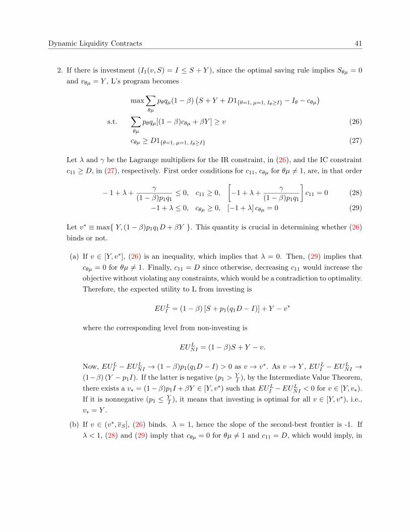
Dynamic Liquidity Contracts 41
2. If there is investment (I1(v, S) = I ≤ S + Y ), since the optimal saving rule implies Sθµ = 0
and vθµ = Y , L’s program becomes
max∑
θµ
pθqµ(1− β)(S + Y +D1{θ=1, µ=1, Iθ≥I} − Iθ − cθµ
)
s.t.∑
θµ
pθqµ[(1− β)cθµ + βY ] ≥ v (26)
cθµ ≥ D1{θ=1, µ=1, Iθ≥I} (27)
Let λ and γ be the Lagrange multipliers for the IR constraint, in (26), and the IC constraint
c11 ≥ D, in (27), respectively. First order conditions for c11, cθµ for θµ 6= 1, are, in that order
− 1 + λ+γ
(1− β)p1q1≤ 0, c11 ≥ 0,
[−1 + λ+
γ
(1− β)p1q1
]c11 = 0 (28)
−1 + λ ≤ 0, cθµ ≥ 0, [−1 + λ] cθµ = 0 (29)
Let v∗ ≡ max{ Y, (1− β)p1q1D+ βY }. This quantity is crucial in determining whether (26)
binds or not.
(a) If v ∈ [Y, v∗], (26) is an inequality, which implies that λ = 0. Then, (29) implies that
cθµ = 0 for θµ 6= 1. Finally, c11 = D since otherwise, decreasing c11 would increase the
objective without violating any constraints, which would be a contradiction to optimality.
Therefore, the expected utility to L from investing is
EULI = (1− β) [S + p1(q1D − I)] + Y − v∗
where the corresponding level from non-investing is
EULNI = (1− β)S + Y − v.
Now, EULI − EULNI → (1− β)p1(q1D − I) > 0 as v → v∗. As v → Y , EULI − EULNI →(1−β) (Y − p1I). If the latter is negative (p1 >
YI ), by the Intermediate Value Theorem,
there exists a v∗ = (1− β)p1I + βY ∈ [Y, v∗) such that EULI −EULNI < 0 for v ∈ [Y, v∗).
If it is nonnegative (p1 ≤ YI ), it means that investing is optimal for all v ∈ [Y, v∗), i.e.,
v∗ = Y .
(b) If v ∈ (v∗, vS ], (26) binds. λ = 1, hence the slope of the second-best frontier is -1. If
λ < 1, (28) and (29) imply that cθµ = 0 for θµ 6= 1 and c11 = D, which would imply, in

42 Onur Ozgur
turn, that v = v∗. But, this latter is a contradiction. Therefore, the expected utility to
L from investing is
EULI = (1− β) [S + p1(q1D − I)] + Y − v
where the corresponding level from non-investing is
EULNI = (1− β)S + Y − v.
So, EULI −EULNI = (1− β)p1(q1D− I) > 0 which makes investing the optimal decision
for all v ∈ (v∗, vS ]
2. The proof of the second part follows the same reasoning and machinery that the first one does.
For that reason, it will be omitted.
Q.E.D.
Dynamic Liquidity Contracts 43
References
Albuquerque, R. and Hopenhayn, H. A. (2004), “Optimal Lending Contracts and Firm Dy-
namics”, Review of Economic Studies, 71, 285-315.
Allen, F. and Gale, D. (1997), “Financial Markets, Intermediaries, and Intertemporal Smooth-
ing”, Journal of Political Economy, 105, 523-546.
Alvarez, F. and Jermann, U. J. (2000), “Efficiency, Equilibrium, and Asset Pricing with Risk
of Default,” Econometrica, 59, 1069-1089.
Atkeson, A. (1991), “International Lending with Moral Hazard and Repudiation”, Econometrica,
59, 1069-1089.
Beck, T., Demirguc-Kunt, A. and Maksimovic, V. (2008), “Financing Patterns Around the
World: Are Small Firms Different?”, Journal of Financial Economics, 89, 467-487.
Berger A. N. and Udell, G. (1994), “Did Risk-Based Capital Allocate Bank Credit and Cause
a Credit Crunch in the U.S.?”, Journal of Money, Credit and Banking, 26, 585-628.
Bernanke, B. S. and Lown, C. S. (1991), “The Credit Crunch,” Brookings Papers on Economic
Activity, 2, 205-247.
Bernanke, B. S. and Gertler, M. (1989), “Agency Cost, Net Worth and Business Fluctua-
tions,” American Economic Review, 79, 14-31.
Besanko, D. and Kanatas, G. (1996), “The Regulation of Bank Capital: Do Capital Standards
Promote Bank Safety?” Journal of Financial Intermediation, 5 (2), 160-183.
Brunnermeier M. and L. H. Pedersen (2009), “Market Liquidity and Funding Liquidity”,
Review of Financial Studies, 22 (6), 2201-2238.
Cooley, T., Marimon R. and Quadrini V. (2004), “Aggregate Consequences of Limited Con-
tract Enforceability”, Journal of Political Economy, 112, 817-847.
Diamond, D. and Dybvig, P. (1983), “Bank Runs, Liquidity, and Deposit Insurance”, Journal
of Political Economy, 91, 401-419.
Diamond, D. and Rajan, R. (2000), “A Theory of Bank Capital,” Journal of Finance, 55,
2431-2465.
44 Onur Ozgur
Holmstrom, B. and Tirole, J. (1997), “Financial Intermediation, Loanable Funds, and the
Real Sector,” Quarterly Journal of Economics, 112, 663-692.
Holmstrom, B. and Tirole, J. (2011), Inside and Outside Liquidity, Cambridge, MA: The MIT
Press.
Hopenhayn, H. and Werning, I. (2008), “Equilibrium Default,” Mimeo, University of California
at Los Angeles.
Hoshi, T., Kashyap, A. and Scharfstein, D. (1990a), “Bank Monitoring and Investment:
Evidence from the Changing Structure of Japanese Corporate Banking Relationships,” in R.
Glenn Hubbard, editor, Asymmetric Information, Corporate Finance and Investment (University
of Chicago Press, Chicago, Illinois).
Hoshi, T., Kashyap, A. and Scharfstein, D. (1990b), “The Role of Banks in Reducing the
Costs of Financial Distress in Japan,” Journal of Financial Economics, 27, 67-88.
Hoshi, T., Kashyap, A. and Scharfstein, D. (1991), “Corporate Structure, Liquidity and
Investment: Evidence from Japanese Industrial Groups,” Quarterly Journal of Economics, 106,
33-60.
James, C. M. (2009), “Credit Market Conditions and the Use of Bank Lines of Credit”, FRBSF
Economic Letter, 2009-27.
Kashyap, A. and Stein, J. (2000), “What do a Million Observations on Banks Say about the
Transmission of Monetary Policy?” American Economic Review, 90 (3), 407-428.
Kehoe, T. J. and Levine, D. K. (1993), “Debt-Constrained Asset Markets,” Review of Economic
Studies, 60, 865-888.
Kovrijnykh, N. (2010), “Debt Contracts with Partial Commitment”, mimeo, Arizona State Uni-
versity.
MacLeod, W. B. and Malcomson, J. (1989), “Implicit Contracts, Incentive Compatibility and
Involuntary Unemployment,” Econometrica, 57, 447-480.
Nikolau, K. (2009), “Liquidity (Risk) Concepts: Definitions and Interactions”, European Central
Bank Working Paper 1008.
Dynamic Liquidity Contracts 45
Petersen, M. and Rajan, R. (1995), “The Effect of Credit Market Competition on Lending
Relationships,” Quarterly Journal of Economics, 110, 407-443.
Phelan, C. (1995), “Repeated Moral Hazard and One-Sided Commitment”, Journal of Economic
Theory, 66, 488-506.
Ray, D. (2002), “The Time Structure of Self-Enforcing Agreements”, Econometrica, 70, 547-582.
Sharpe, S. (1995), “Bank Capitalization, Regulation, and the Credit Crunch: A Critical Review
of the Research Findings.” Finance and Economics Discussion Series paper No. 95/20, Board of
Governors of the Federal Reserve System.
Stokey, N. L. and Lucas, R. E. (with Prescott, E. C.) (1989), Recursive Methods in
Economic Dynamics, Cambridge, MA: Harvard University Press.
Sufi, A. (2009), “Bank Lines of Credit in Corporate Finance: An Empirical Analysis”, Review of
Financial Studies, 22 (3), 1057-1088.
Sundaram, R. K. (1996), A First Course in Optimization Theory, Cambridge, Cambridge Uni-
versity Press.
Thakor, A. (1996), “Capital Requirements, Monetary Policy, and Aggregate Bank Lending: The-
ory and Empirical Evidence,” Journal of Finance, 51 (1), 279-324.
Thomas, J. and Worrall, T. (1994), “Foreign Direct Investment and the Risk of Expropria-
tion”, Review of Economic Studies, 61, 81-108.
Thomas, J. and Worrall, T. (2010), “Dynamic Relational Contracts with Credit Constraints”,
mimeo, University of Manchester.
von Thadden, E-L. (2004), “Liquidity”, in S. Bhattacharya, A. Boot, A. Thakor (eds.): Credit,
Intermediation, and the Macroeconomy, Oxford University Press, 249-261.

![LISTADO DE JUEGOS - PinillaNumero Descripcion Foto 291 [NDS]Artic_Tale[EUR] 798 [NDS]Asphalt_Urban_GT_2[EUR] 306 [NDS]Assassins_Creed_Altairs_Chronicles[EUR] 285 [NDS]Assassins_Creed_Altairs_Chronicles[USA]](https://img.pdfslide.us/doc/110x75/5f07ebef7e708231d41f6db4/listado-de-juegos-numero-descripcion-foto-291-ndsartictaleeur-798-ndsasphalturbangt2eur.jpg)