Embed Size (px)
Citation preview
E-mail: [email protected]://web.yonsei.ac.kr/hgjung
6. Linear Transformations6. Linear Transformations
E-mail: [email protected]://web.yonsei.ac.kr/hgjung
6.1. Matrices as Transformations6.1. Matrices as Transformations
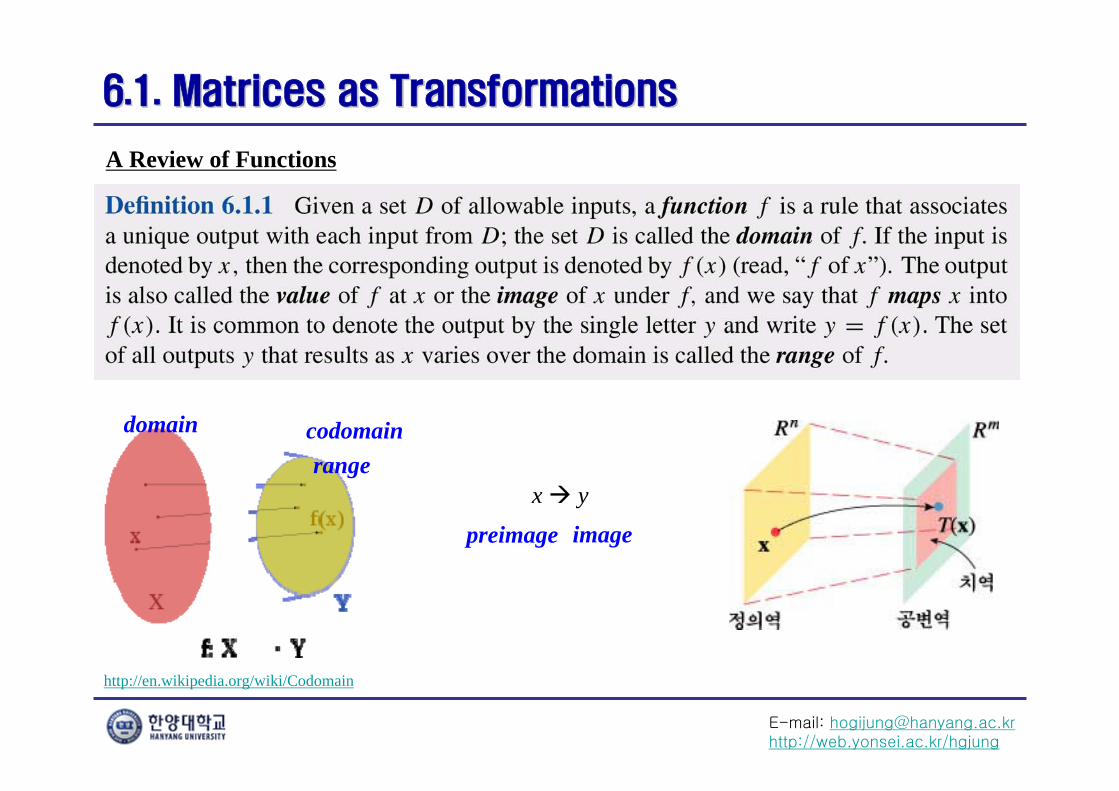
A Review of Functions
http://en.wikipedia.org/wiki/Codomain
domain codomainrange
x y
imagepreimage
E-mail: [email protected]://web.yonsei.ac.kr/hgjung
6.1. Matrices as Transformations6.1. Matrices as Transformations
A Review of Functions
A function whose input and outputs are vectors is called a transformation, and it is standard to denote transformations by capital letters such as F, T, or L.
w=T(x)
“T maps x into w”
E-mail: [email protected]://web.yonsei.ac.kr/hgjung
6.1. Matrices as Transformations6.1. Matrices as Transformations
A Review of Functions
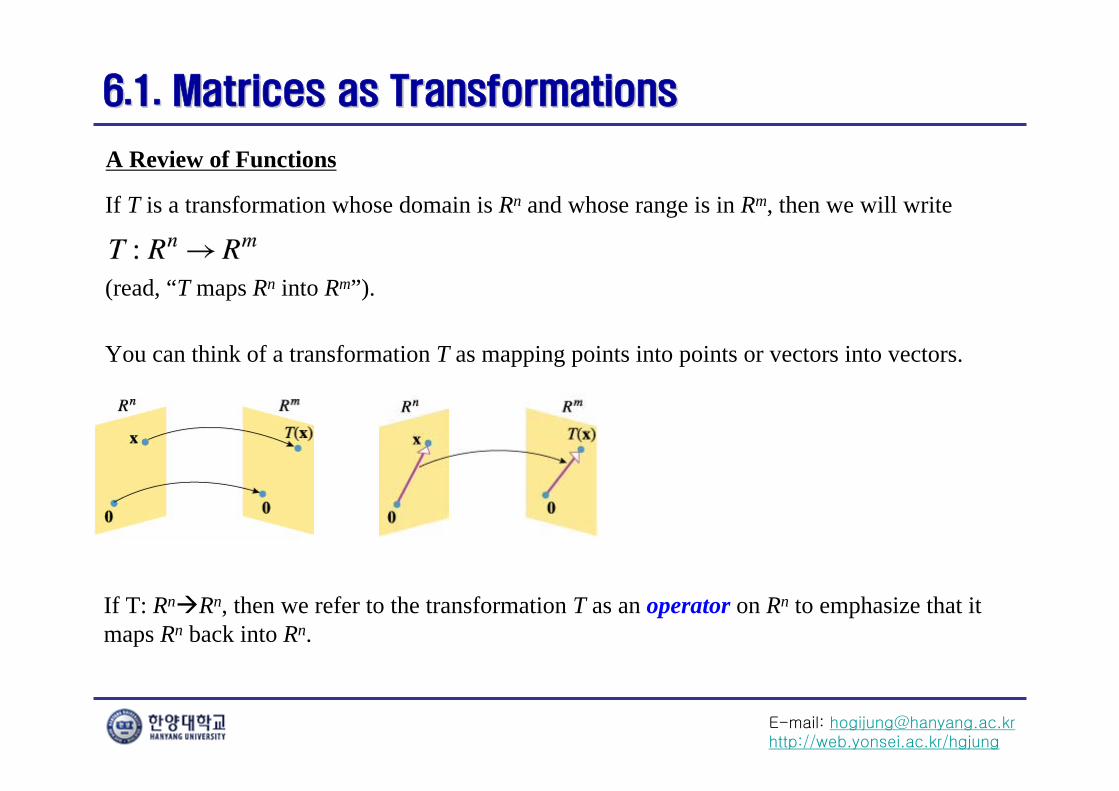
If T is a transformation whose domain is Rn and whose range is in Rm, then we will write
You can think of a transformation T as mapping points into points or vectors into vectors.
(read, “T maps Rn into Rm”).
If T: RnRn, then we refer to the transformation T as an operator on Rn to emphasize that it maps Rn back into Rn.
E-mail: [email protected]://web.yonsei.ac.kr/hgjung
6.1. Matrices as Transformations6.1. Matrices as Transformations
Matrix Transformations
Matrix transformation
If A is an m×n matrix, and if x is a column vector in Rn, then the product Ax is a vector in Rm, so multiplying x by A creates a transformation that maps vectors in Rn into vectors in Rm. We call this transformation multiplication by A or the transformation A and denote it by TA to emphasize the matrix A.
and
or equivalently,
In the special case where A is square, say n×n, we have ,
and we call TA a matrix operator on Rn.
: n nAT R R
E-mail: [email protected]://web.yonsei.ac.kr/hgjung
6.1. Matrices as Transformations6.1. Matrices as Transformations
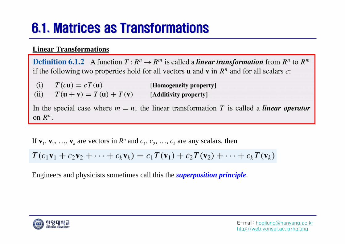
Linear Transformations
The operational interpretation of linearity
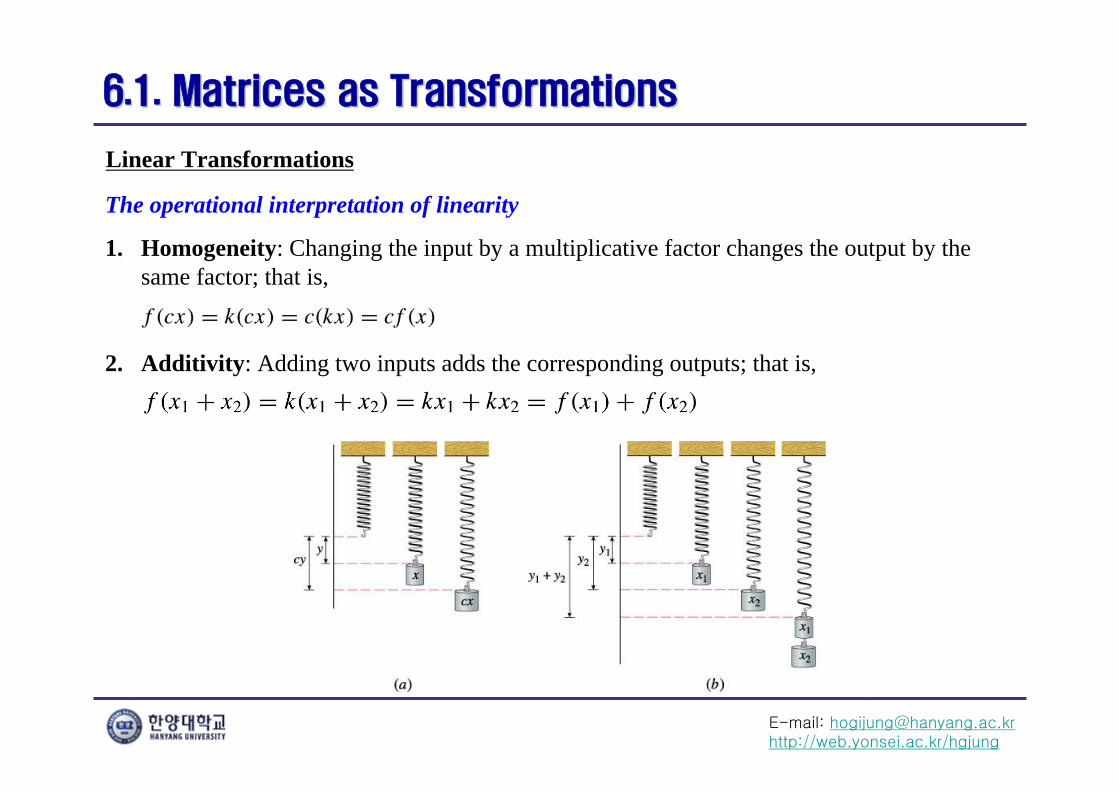
1. Homogeneity: Changing the input by a multiplicative factor changes the output by the same factor; that is,
2. Additivity: Adding two inputs adds the corresponding outputs; that is,
E-mail: [email protected]://web.yonsei.ac.kr/hgjung
6.1. Matrices as Transformations6.1. Matrices as Transformations
Linear Transformations
If v1, v2, …, vk are vectors in Rn and c1, c2, …, ck are any scalars, then
Engineers and physicists sometimes call this the superposition principle.
E-mail: [email protected]://web.yonsei.ac.kr/hgjung
6.1. Matrices as Transformations6.1. Matrices as Transformations
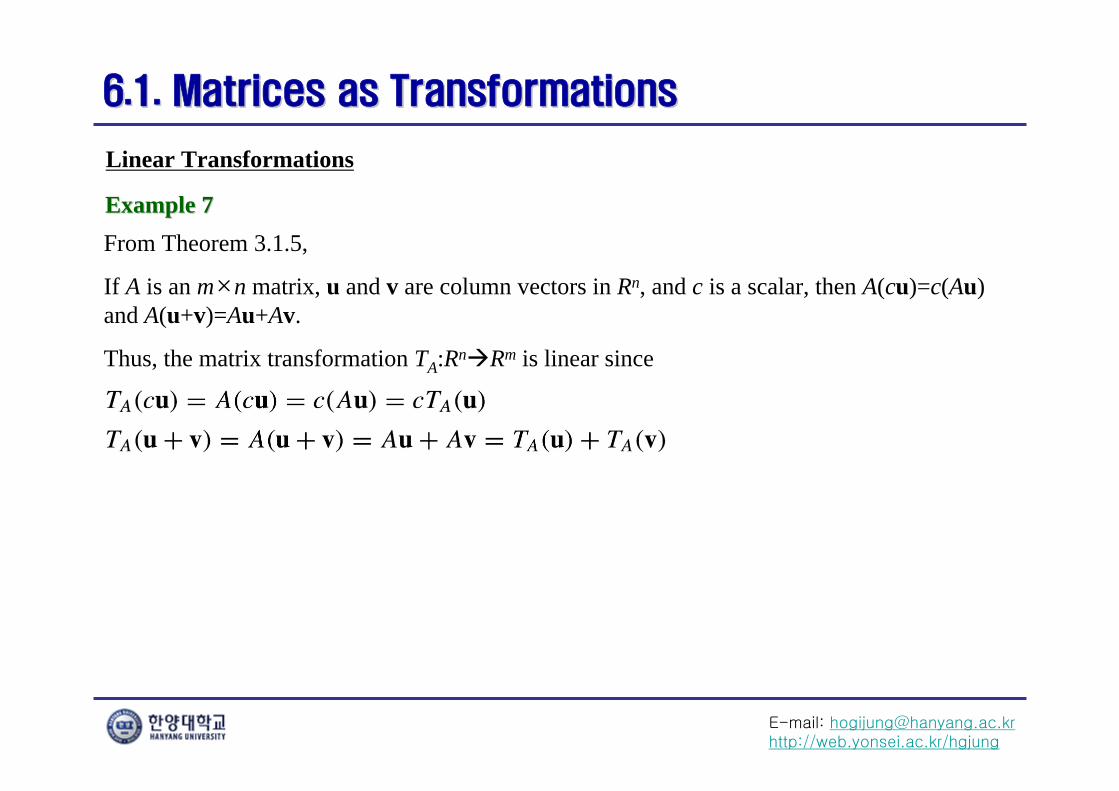
Linear Transformations
Example 7Example 7From Theorem 3.1.5,
If A is an m×n matrix, u and v are column vectors in Rn, and c is a scalar, then A(cu)=c(Au) and A(u+v)=Au+Av.
Thus, the matrix transformation TA:RnRm is linear since
E-mail: [email protected]://web.yonsei.ac.kr/hgjung
6.1. Matrices as Transformations6.1. Matrices as Transformations
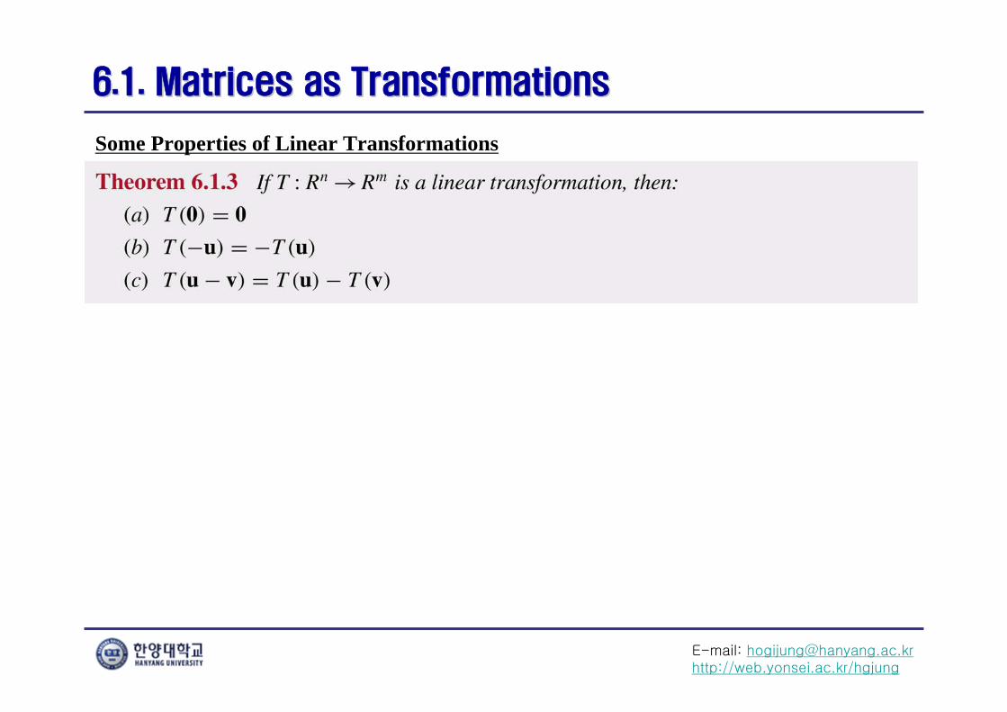
Some Properties of Linear Transformations
E-mail: [email protected]://web.yonsei.ac.kr/hgjung
6.1. Matrices as Transformations6.1. Matrices as Transformations
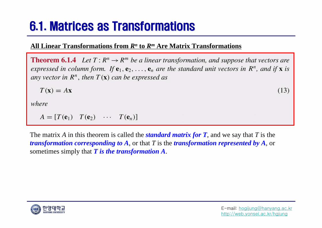
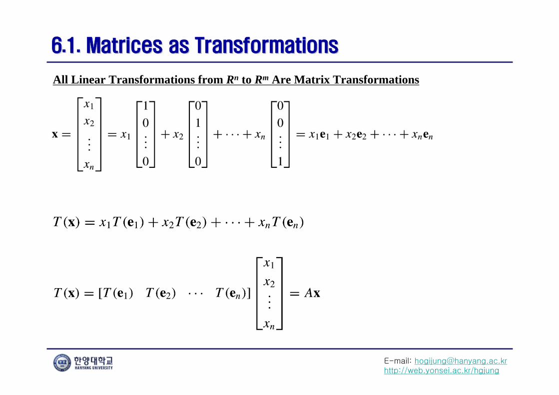
All Linear Transformations from Rn to Rm Are Matrix Transformations
The matrix A in this theorem is called the standard matrix for T, and we say that T is the transformation corresponding to A, or that T is the transformation represented by A, or sometimes simply that T is the transformation A.
E-mail: [email protected]://web.yonsei.ac.kr/hgjung
6.1. Matrices as Transformations6.1. Matrices as Transformations
All Linear Transformations from Rn to Rm Are Matrix Transformations
E-mail: [email protected]://web.yonsei.ac.kr/hgjung
6.1. Matrices as Transformations6.1. Matrices as Transformations
All Linear Transformations from Rn to Rm Are Matrix Transformations
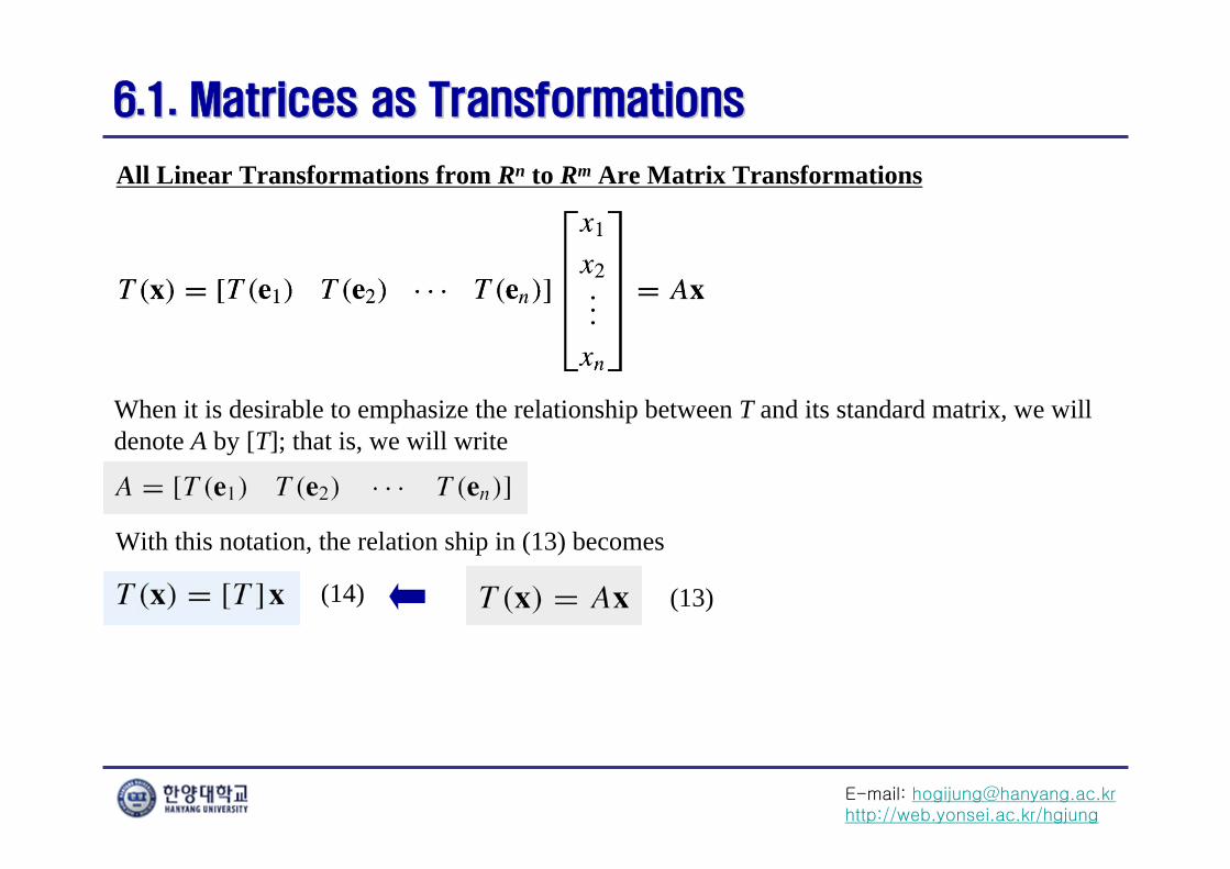
When it is desirable to emphasize the relationship between T and its standard matrix, we will denote A by [T]; that is, we will write
With this notation, the relation ship in (13) becomes
(14) (13)
E-mail: [email protected]://web.yonsei.ac.kr/hgjung
6.1. Matrices as Transformations6.1. Matrices as Transformations
All Linear Transformations from Rn to Rm Are Matrix Transformations
REMARK
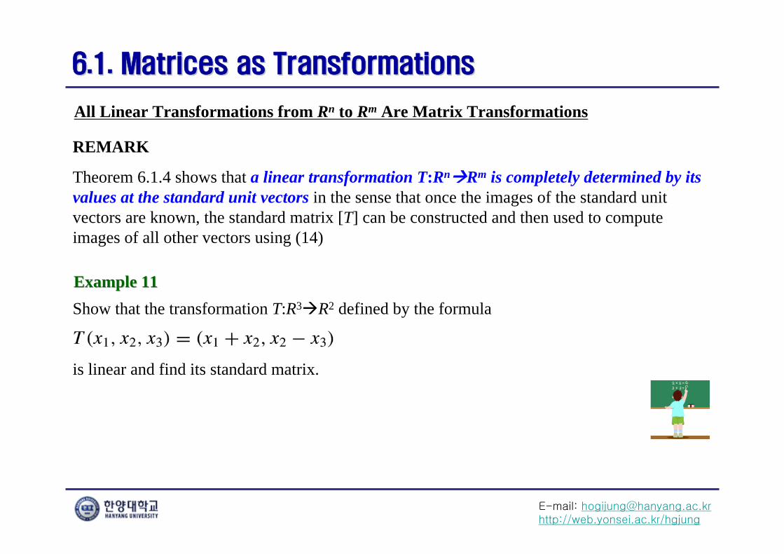
Theorem 6.1.4 shows that a linear transformation T:RnRm is completely determined by its values at the standard unit vectors in the sense that once the images of the standard unit vectors are known, the standard matrix [T] can be constructed and then used to compute images of all other vectors using (14)
Example 11Example 11Show that the transformation T:R3R2 defined by the formula
is linear and find its standard matrix.
E-mail: [email protected]://web.yonsei.ac.kr/hgjung
6.1. Matrices as Transformations6.1. Matrices as Transformations
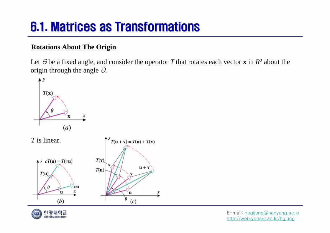
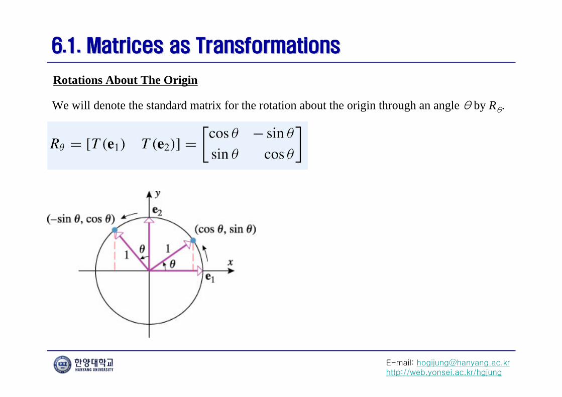
Rotations About The Origin
Let θ be a fixed angle, and consider the operator T that rotates each vector x in R2 about the origin through the angle θ.
T is linear.
E-mail: [email protected]://web.yonsei.ac.kr/hgjung
6.1. Matrices as Transformations6.1. Matrices as Transformations
Rotations About The Origin
We will denote the standard matrix for the rotation about the origin through an angle θ by Rθ.
E-mail: [email protected]://web.yonsei.ac.kr/hgjung
6.1. Matrices as Transformations6.1. Matrices as Transformations
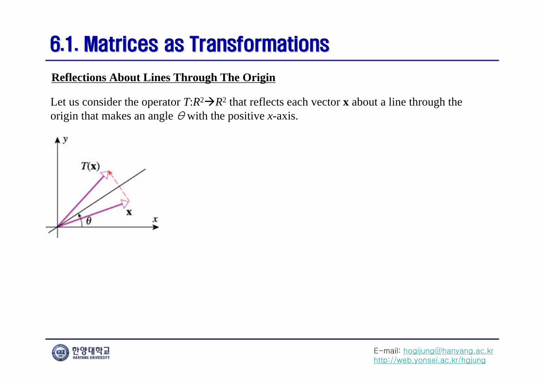
Reflections About Lines Through The Origin
Let us consider the operator T:R2R2 that reflects each vector x about a line through the origin that makes an angle θ with the positive x-axis.
E-mail: [email protected]://web.yonsei.ac.kr/hgjung
6.1. Matrices as Transformations6.1. Matrices as Transformations
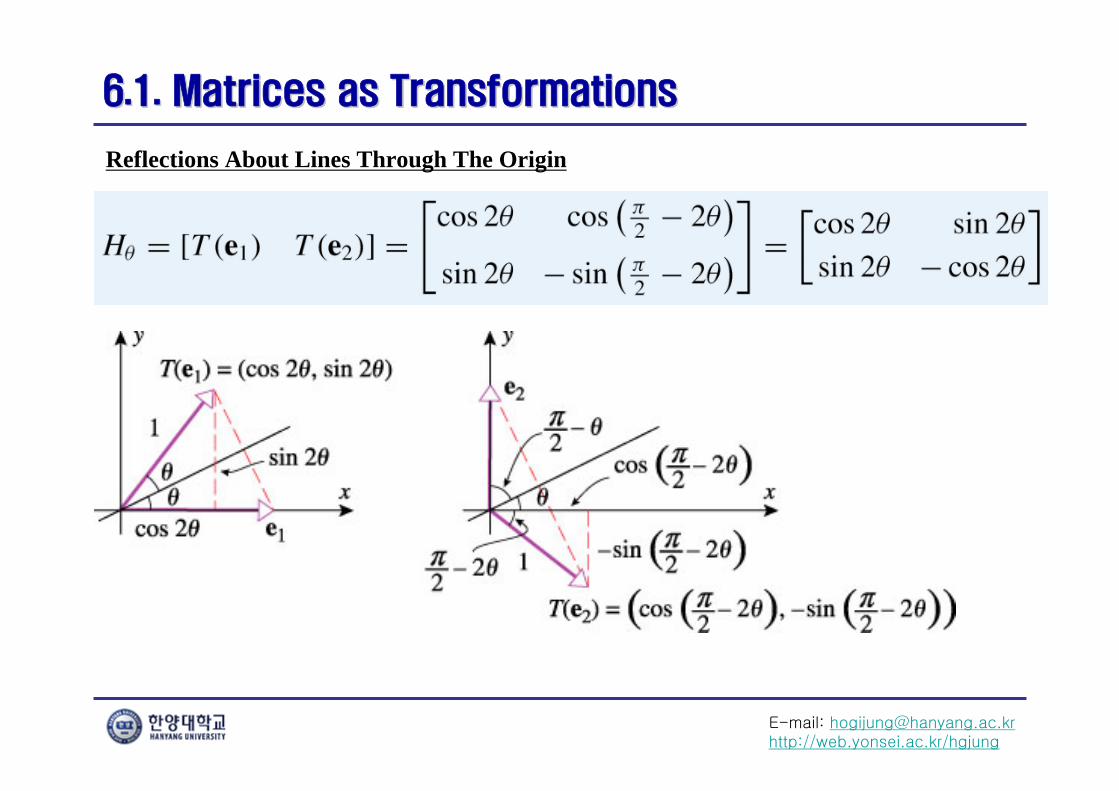
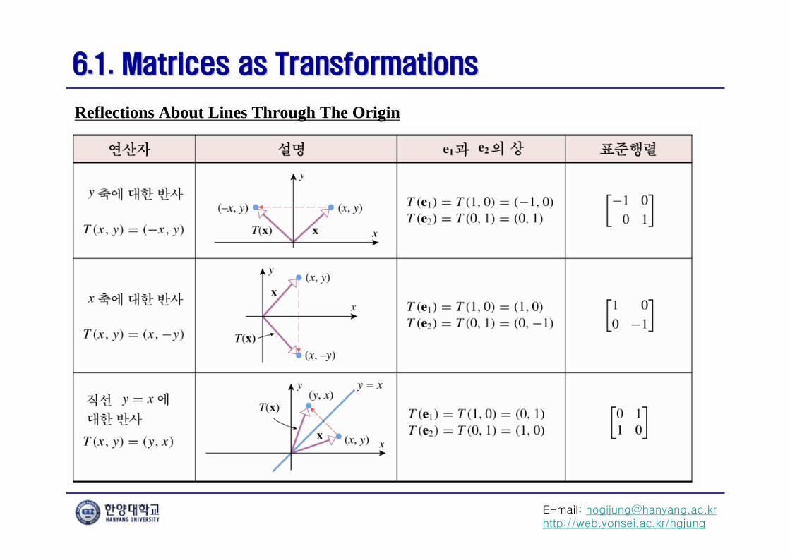
Reflections About Lines Through The Origin
E-mail: [email protected]://web.yonsei.ac.kr/hgjung
6.1. Matrices as Transformations6.1. Matrices as Transformations
Reflections About Lines Through The Origin
E-mail: [email protected]://web.yonsei.ac.kr/hgjung
6.1. Matrices as Transformations6.1. Matrices as Transformations
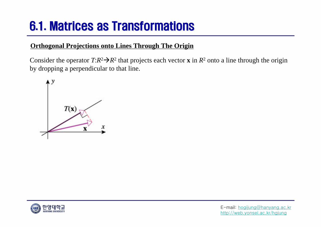
Orthogonal Projections onto Lines Through The Origin
Consider the operator T:R2R2 that projects each vector x in R2 onto a line through the origin by dropping a perpendicular to that line.
E-mail: [email protected]://web.yonsei.ac.kr/hgjung
6.1. Matrices as Transformations6.1. Matrices as Transformations
Orthogonal Projections onto Lines Through The Origin
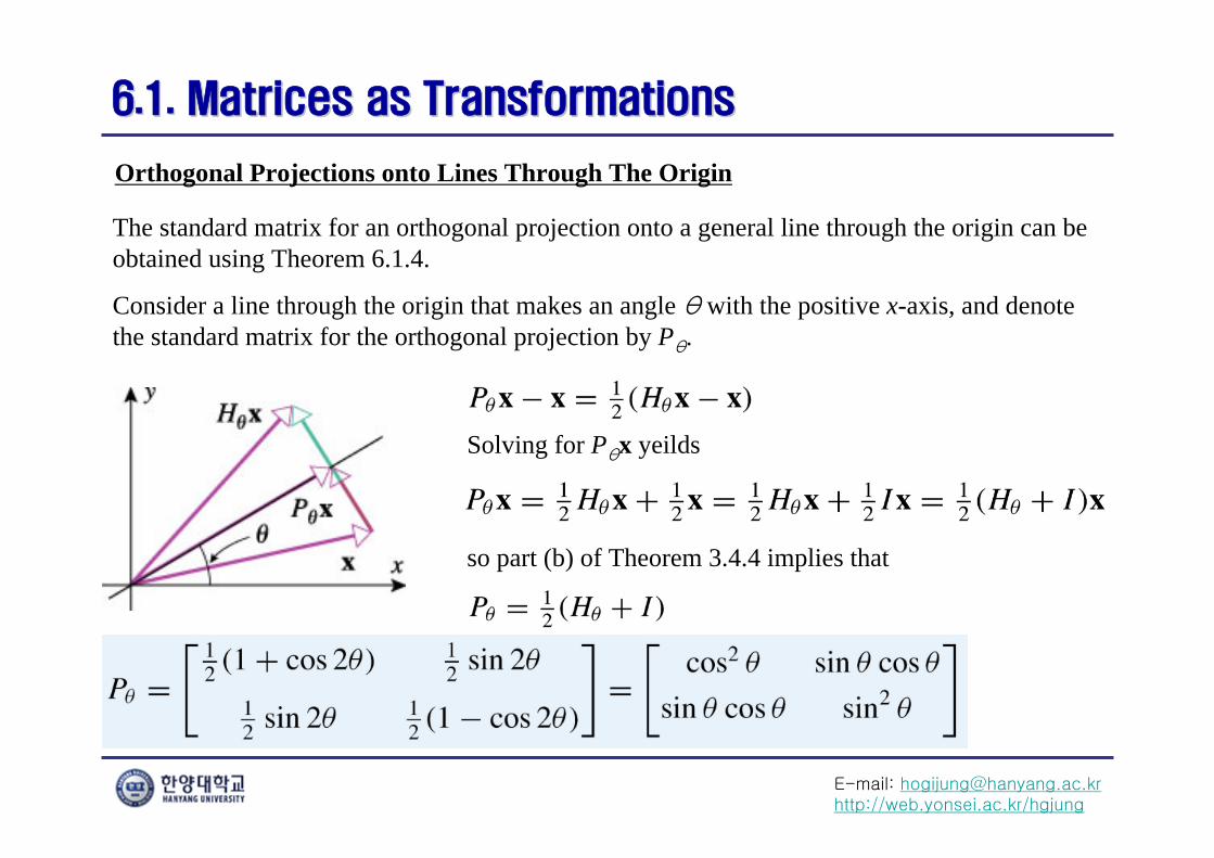
The standard matrix for an orthogonal projection onto a general line through the origin can be obtained using Theorem 6.1.4.
Consider a line through the origin that makes an angle θ with the positive x-axis, and denote the standard matrix for the orthogonal projection by Pθ.
Solving for Pθx yeilds
so part (b) of Theorem 3.4.4 implies that
E-mail: [email protected]://web.yonsei.ac.kr/hgjung
6.1. Matrices as Transformations6.1. Matrices as Transformations
Orthogonal Projections onto Lines Through The Origin
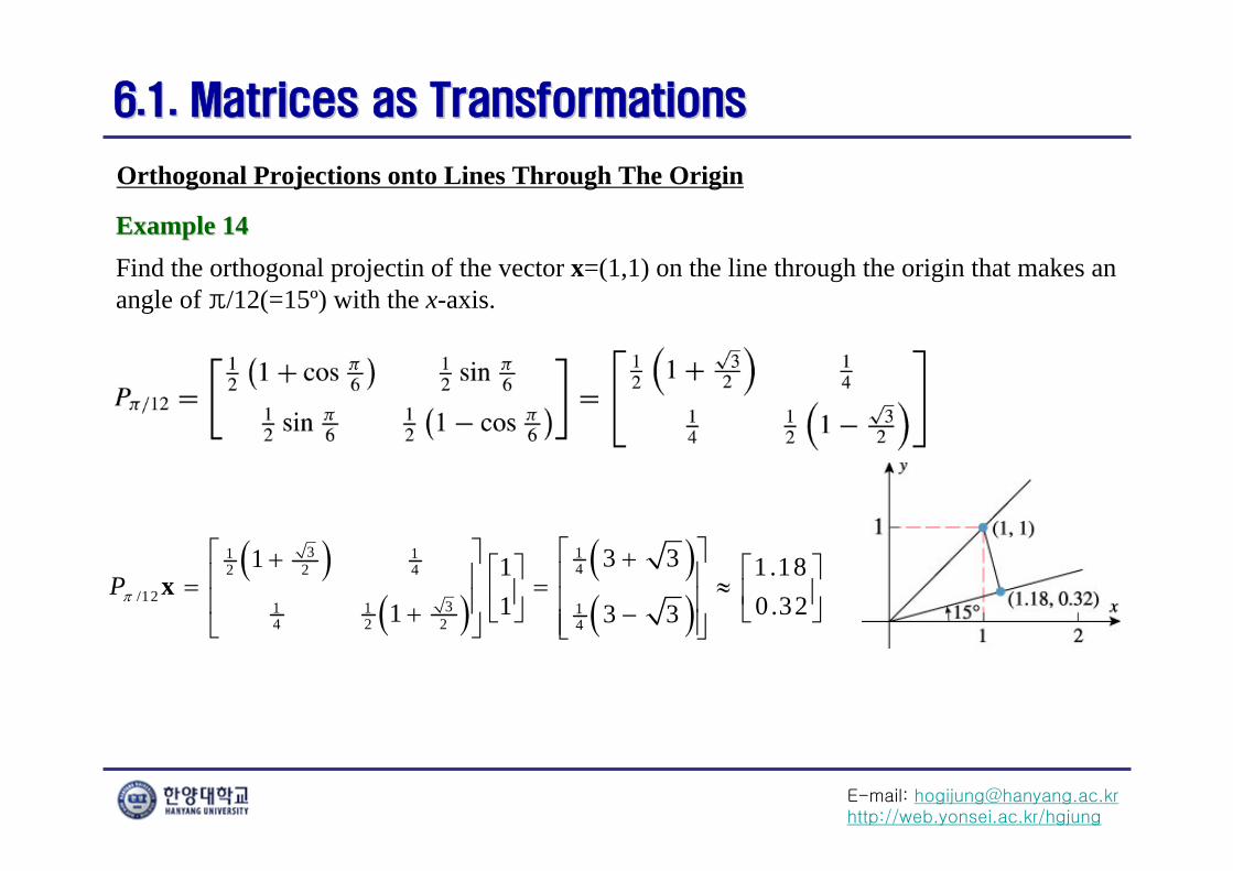
Find the orthogonal projectin of the vector x=(1,1) on the line through the origin that makes an angle of π/12(=15º) with the x-axis.
Example 14Example 14
3 11 142 2 4
/1231 1 1
4 2 2 4
3 31 1 1.181 0.321 3 3
P
x
E-mail: [email protected]://web.yonsei.ac.kr/hgjung
6.1. Matrices as Transformations6.1. Matrices as Transformations
Orthogonal Projections onto Lines Through The Origin
E-mail: [email protected]://web.yonsei.ac.kr/hgjung
6.1. Matrices as Transformations6.1. Matrices as Transformations
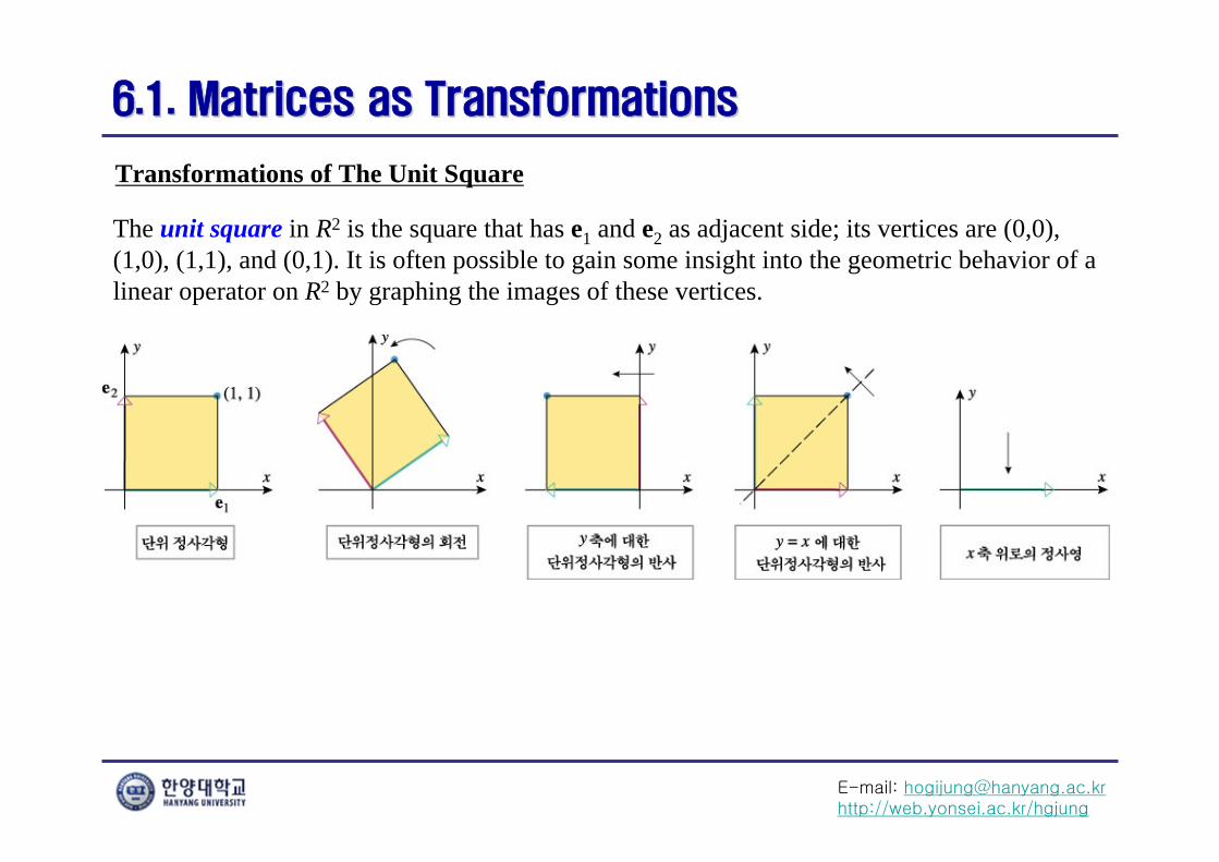
Transformations of The Unit Square
The unit square in R2 is the square that has e1 and e2 as adjacent side; its vertices are (0,0), (1,0), (1,1), and (0,1). It is often possible to gain some insight into the geometric behavior of a linear operator on R2 by graphing the images of these vertices.
E-mail: [email protected]://web.yonsei.ac.kr/hgjung
6.2. Geometry of Linear Operators6.2. Geometry of Linear Operators
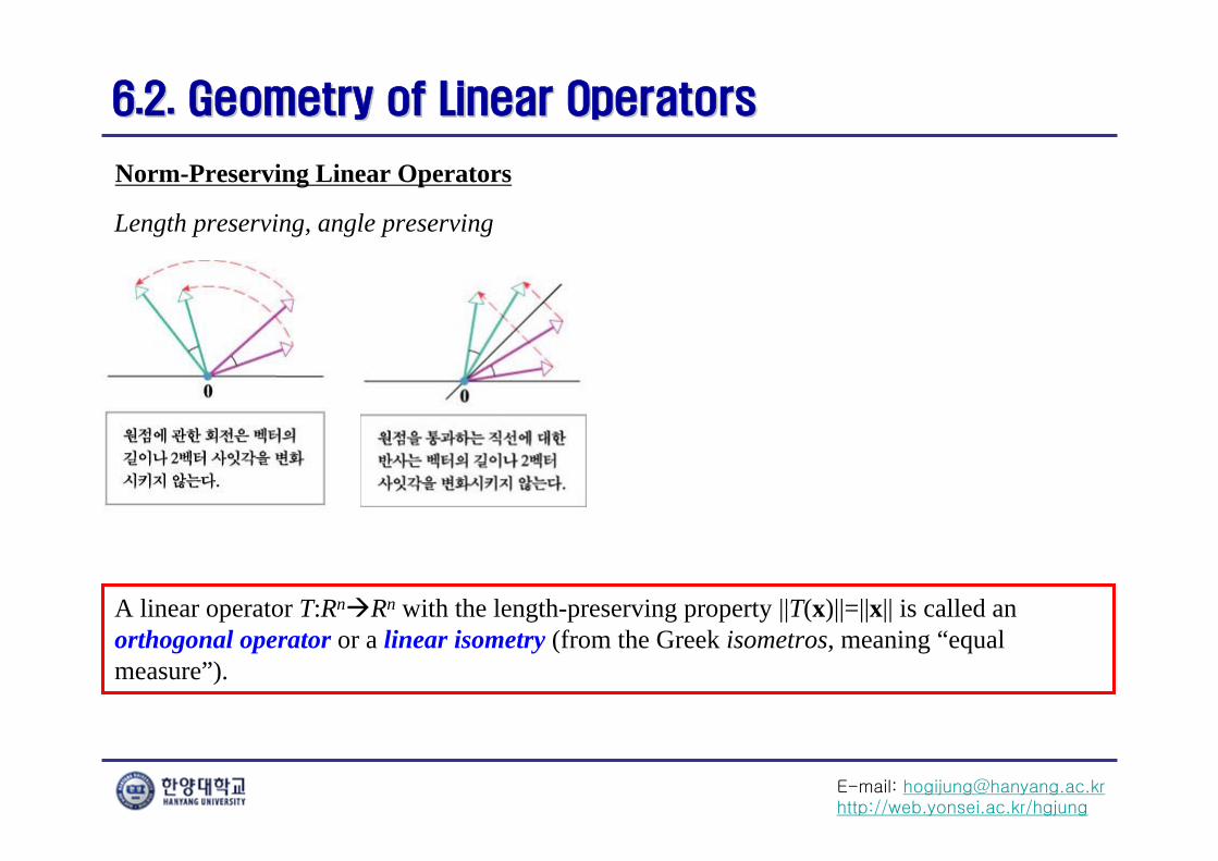
Norm-Preserving Linear Operators
Length preserving, angle preserving
A linear operator T:RnRn with the length-preserving property ||T(x)||=||x|| is called an orthogonal operator or a linear isometry (from the Greek isometros, meaning “equal measure”).
E-mail: [email protected]://web.yonsei.ac.kr/hgjung
6.2. Geometry of Linear Operators6.2. Geometry of Linear Operators
Norm-Preserving Linear Operators
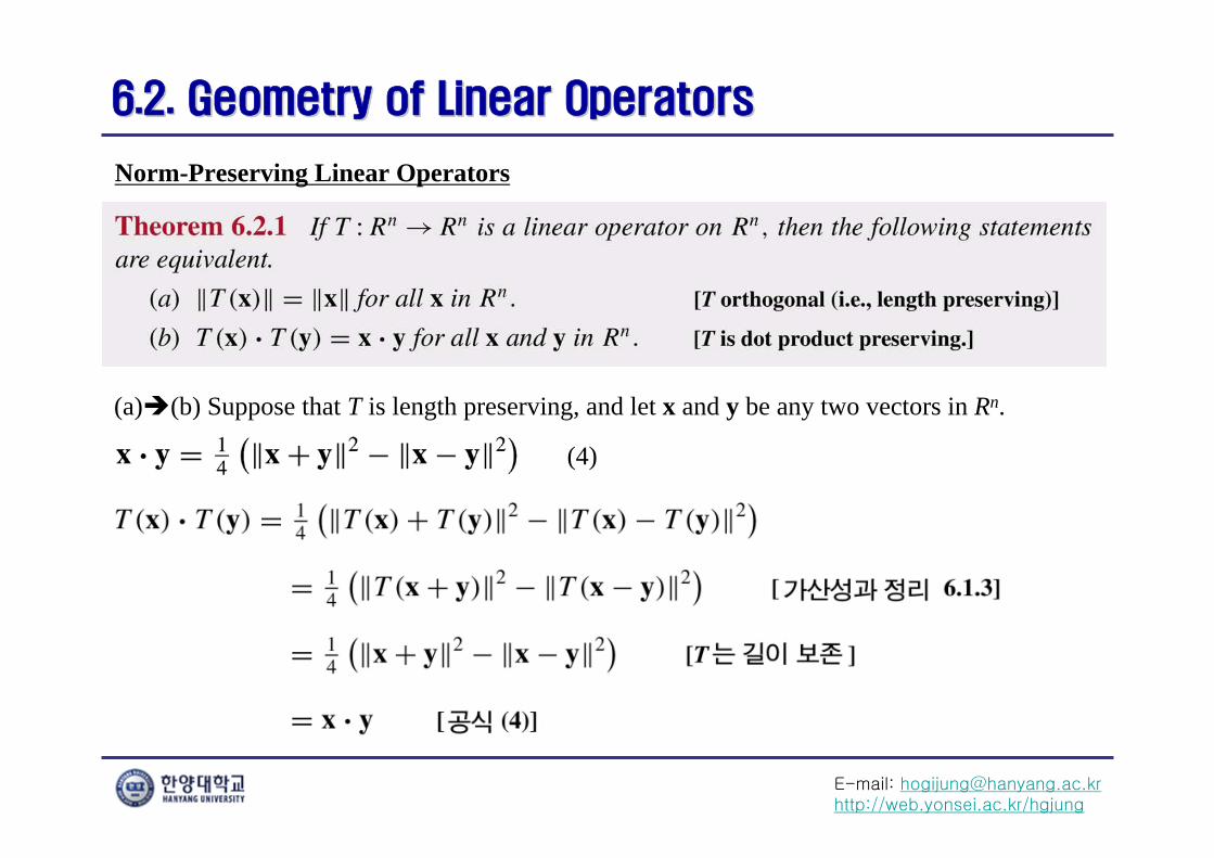
(a)(b) Suppose that T is length preserving, and let x and y be any two vectors in Rn.
(4)
E-mail: [email protected]://web.yonsei.ac.kr/hgjung
6.2. Geometry of Linear Operators6.2. Geometry of Linear Operators
Norm-Preserving Linear Operators
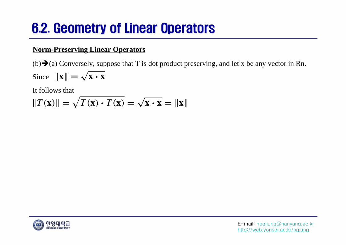
(b)(a) Conversely, suppose that T is dot product preserving, and let x be any vector in Rn.
Since
It follows that
E-mail: [email protected]://web.yonsei.ac.kr/hgjung
6.2. Geometry of Linear Operators6.2. Geometry of Linear Operators
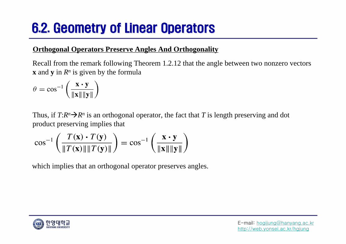
Orthogonal Operators Preserve Angles And Orthogonality
Recall from the remark following Theorem 1.2.12 that the angle between two nonzero vectors x and y in Rn is given by the formula
Thus, if T:RnRn is an orthogonal operator, the fact that T is length preserving and dot product preserving implies that
which implies that an orthogonal operator preserves angles.
E-mail: [email protected]://web.yonsei.ac.kr/hgjung
6.2. Geometry of Linear Operators6.2. Geometry of Linear Operators
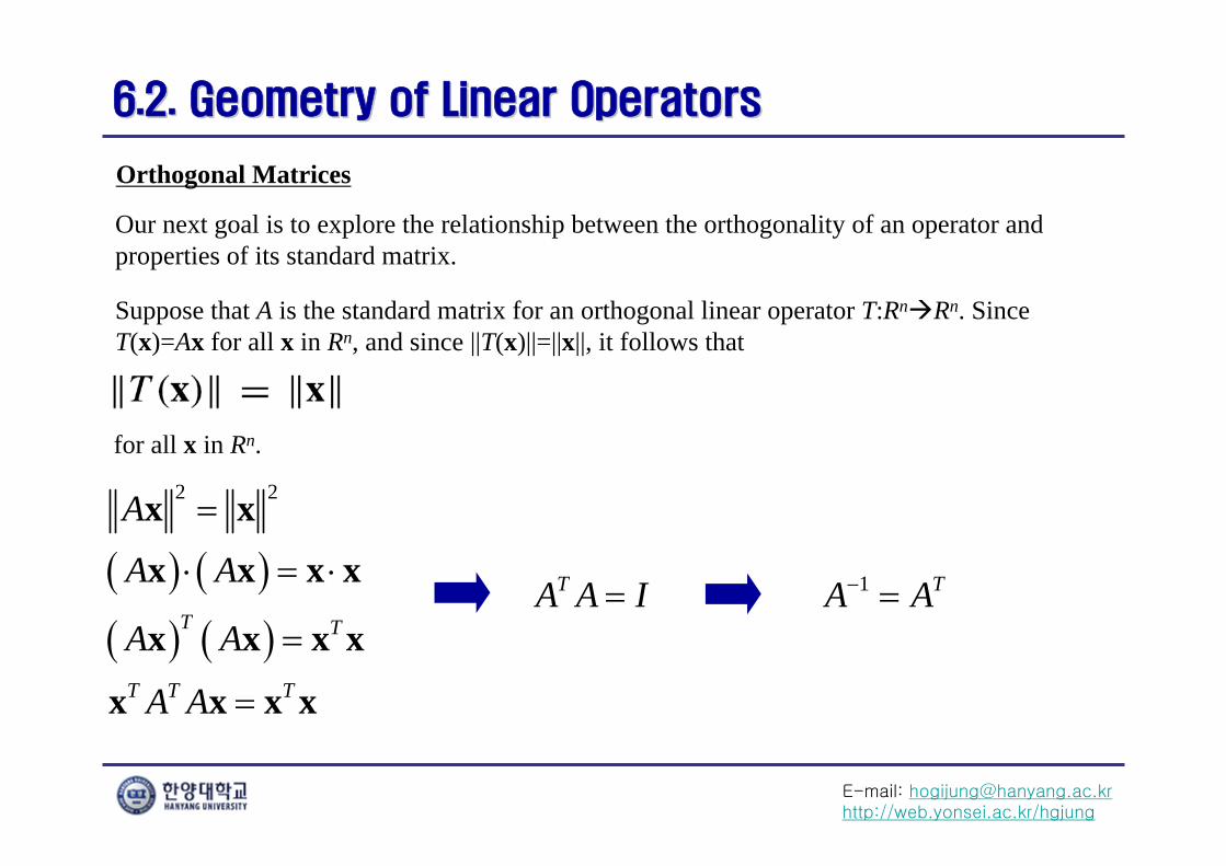
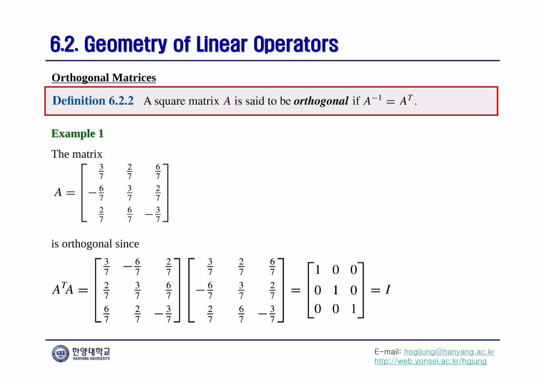
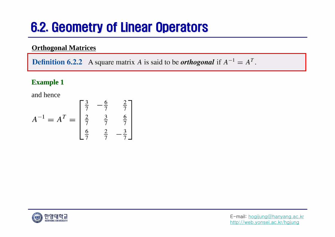
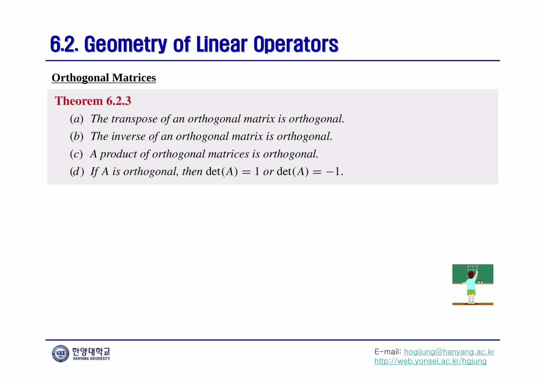
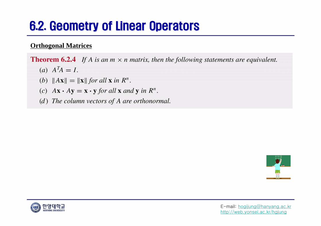
Orthogonal Matrices
Our next goal is to explore the relationship between the orthogonality of an operator and properties of its standard matrix.
Suppose that A is the standard matrix for an orthogonal linear operator T:RnRn. Since T(x)=Ax for all x in Rn, and since ||T(x)||=||x||, it follows that
for all x in Rn.
2 2
T T
T T T
A
A A
A A
A A
x x
x x x x
x x x x
x x x x
TA A I 1 TA A
E-mail: [email protected]://web.yonsei.ac.kr/hgjung
6.2. Geometry of Linear Operators6.2. Geometry of Linear Operators
Orthogonal Matrices
The matrix
Example 1Example 1
is orthogonal since
E-mail: [email protected]://web.yonsei.ac.kr/hgjung
6.2. Geometry of Linear Operators6.2. Geometry of Linear Operators
Orthogonal Matrices
and hence
Example 1Example 1
E-mail: [email protected]://web.yonsei.ac.kr/hgjung
6.2. Geometry of Linear Operators6.2. Geometry of Linear Operators
Orthogonal Matrices
E-mail: [email protected]://web.yonsei.ac.kr/hgjung
6.2. Geometry of Linear Operators6.2. Geometry of Linear Operators
Orthogonal Matrices
E-mail: [email protected]://web.yonsei.ac.kr/hgjung
6.2. Geometry of Linear Operators6.2. Geometry of Linear Operators
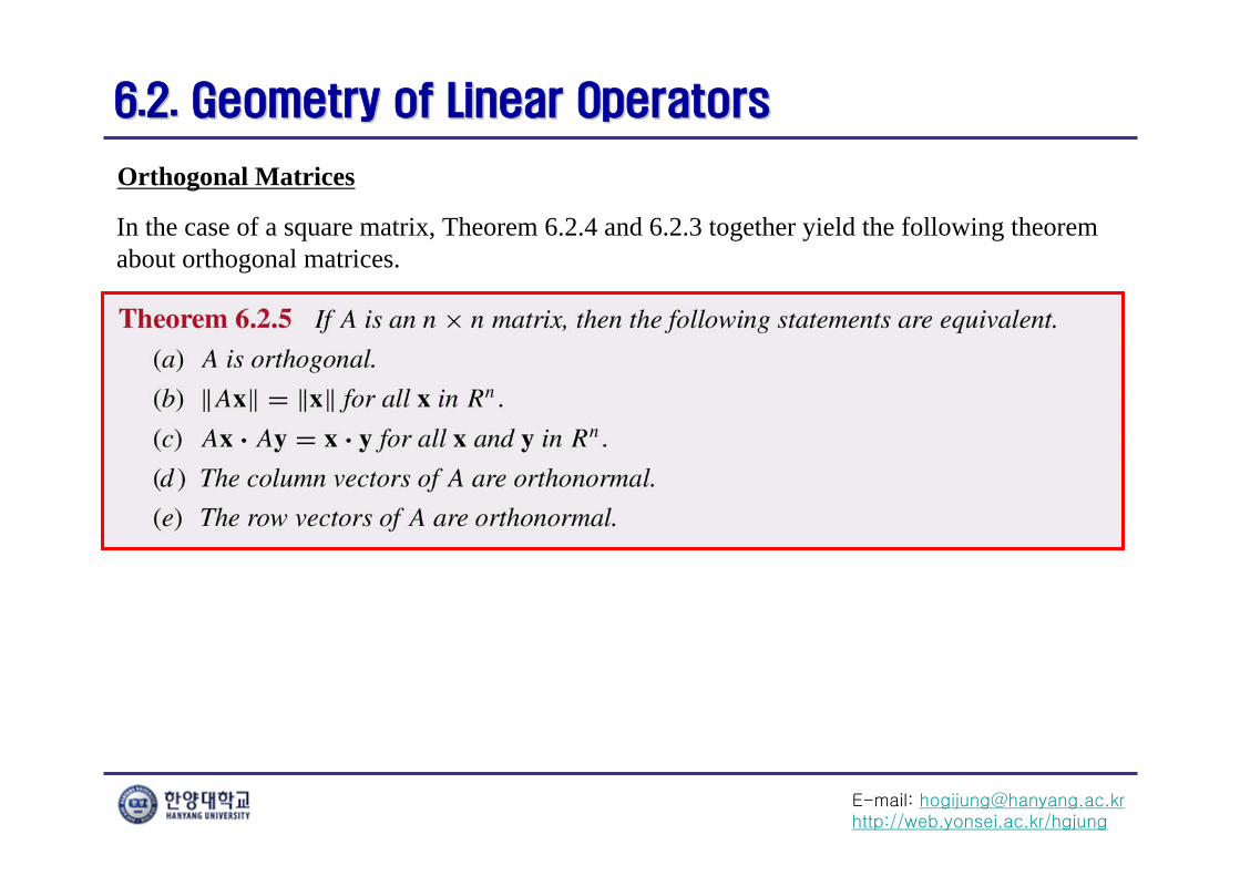
Orthogonal Matrices
In the case of a square matrix, Theorem 6.2.4 and 6.2.3 together yield the following theorem about orthogonal matrices.
E-mail: [email protected]://web.yonsei.ac.kr/hgjung
6.2. Geometry of Linear Operators6.2. Geometry of Linear Operators
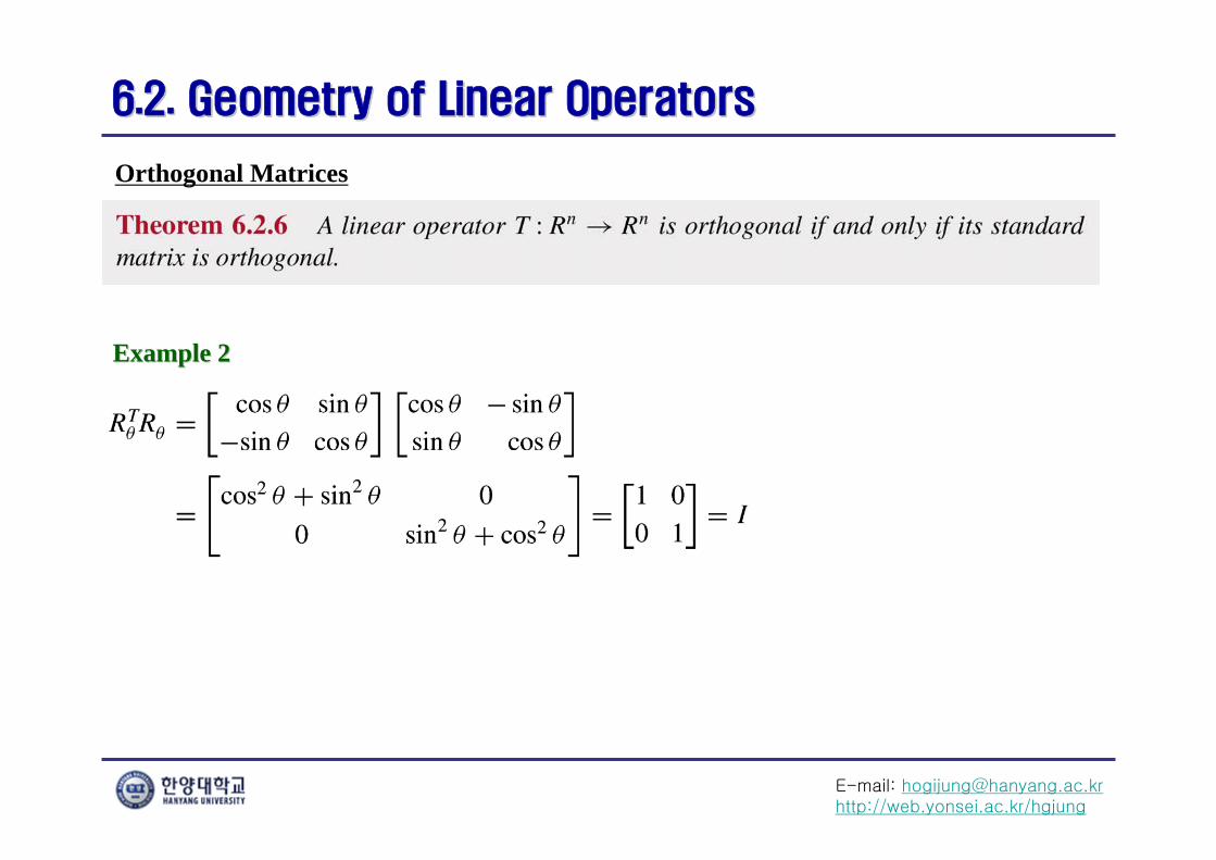
Orthogonal Matrices
Example 2Example 2
E-mail: [email protected]://web.yonsei.ac.kr/hgjung
6.2. Geometry of Linear Operators6.2. Geometry of Linear Operators
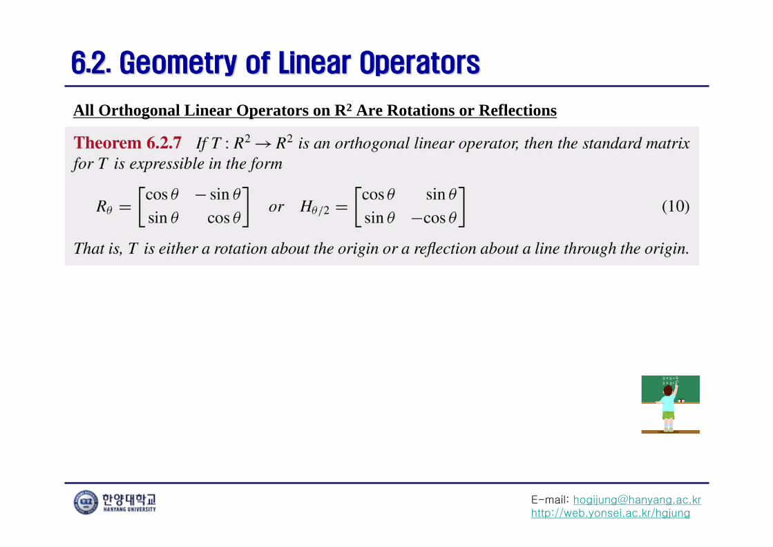
All Orthogonal Linear Operators on R2 Are Rotations or Reflections
E-mail: [email protected]://web.yonsei.ac.kr/hgjung
6.2. Geometry of Linear Operators6.2. Geometry of Linear Operators
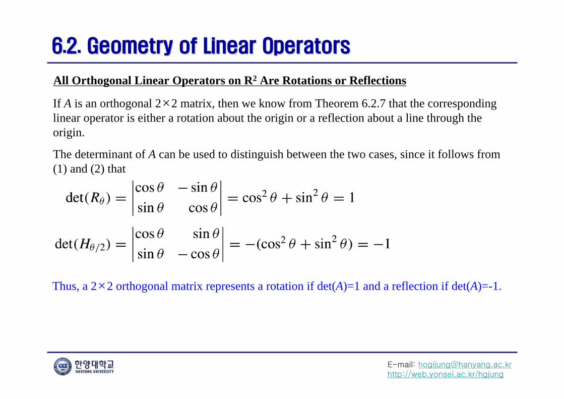
All Orthogonal Linear Operators on R2 Are Rotations or Reflections
If A is an orthogonal 2×2 matrix, then we know from Theorem 6.2.7 that the correspondinglinear operator is either a rotation about the origin or a reflection about a line through the origin.
The determinant of A can be used to distinguish between the two cases, since it follows from (1) and (2) that
Thus, a 2×2 orthogonal matrix represents a rotation if det(A)=1 and a reflection if det(A)=-1.
E-mail: [email protected]://web.yonsei.ac.kr/hgjung
6.2. Geometry of Linear Operators6.2. Geometry of Linear Operators
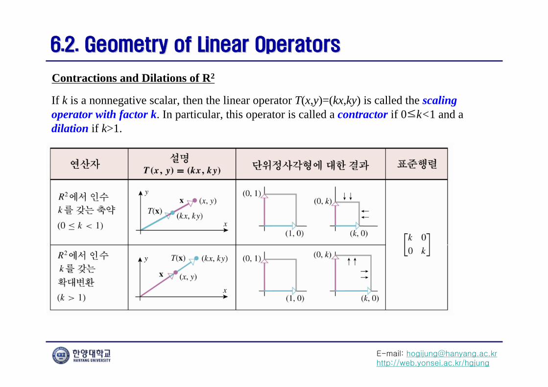
Contractions and Dilations of R2
If k is a nonnegative scalar, then the linear operator T(x,y)=(kx,ky) is called the scaling operator with factor k. In particular, this operator is called a contractor if 0≤k<1 and a dilation if k>1.
E-mail: [email protected]://web.yonsei.ac.kr/hgjung
6.2. Geometry of Linear Operators6.2. Geometry of Linear Operators
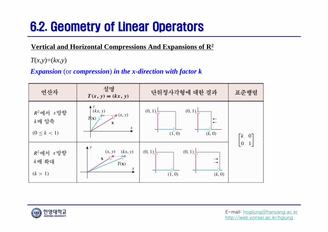
Vertical and Horizontal Compressions And Expansions of R2
Expansion (or compression) in the x-direction with factor kT(x,y)=(kx,y)
E-mail: [email protected]://web.yonsei.ac.kr/hgjung
6.2. Geometry of Linear Operators6.2. Geometry of Linear Operators
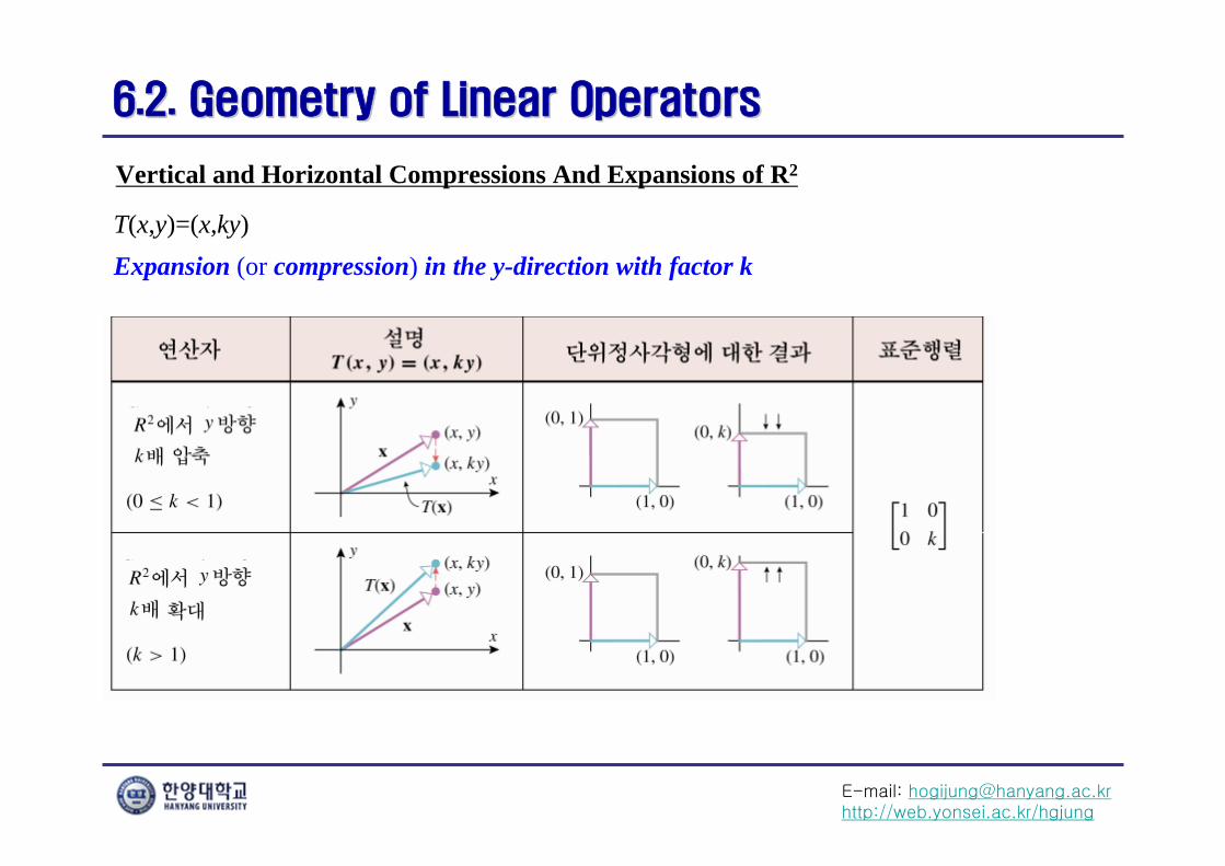
Vertical and Horizontal Compressions And Expansions of R2
Expansion (or compression) in the y-direction with factor kT(x,y)=(x,ky)
E-mail: [email protected]://web.yonsei.ac.kr/hgjung
6.2. Geometry of Linear Operators6.2. Geometry of Linear Operators
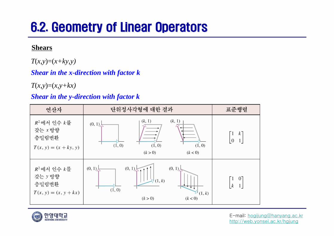
Shears
Shear in the x-direction with factor kT(x,y)=(x+ky,y)
T(x,y)=(x,y+kx)Shear in the y-direction with factor k
E-mail: [email protected]://web.yonsei.ac.kr/hgjung
6.2. Geometry of Linear Operators6.2. Geometry of Linear Operators
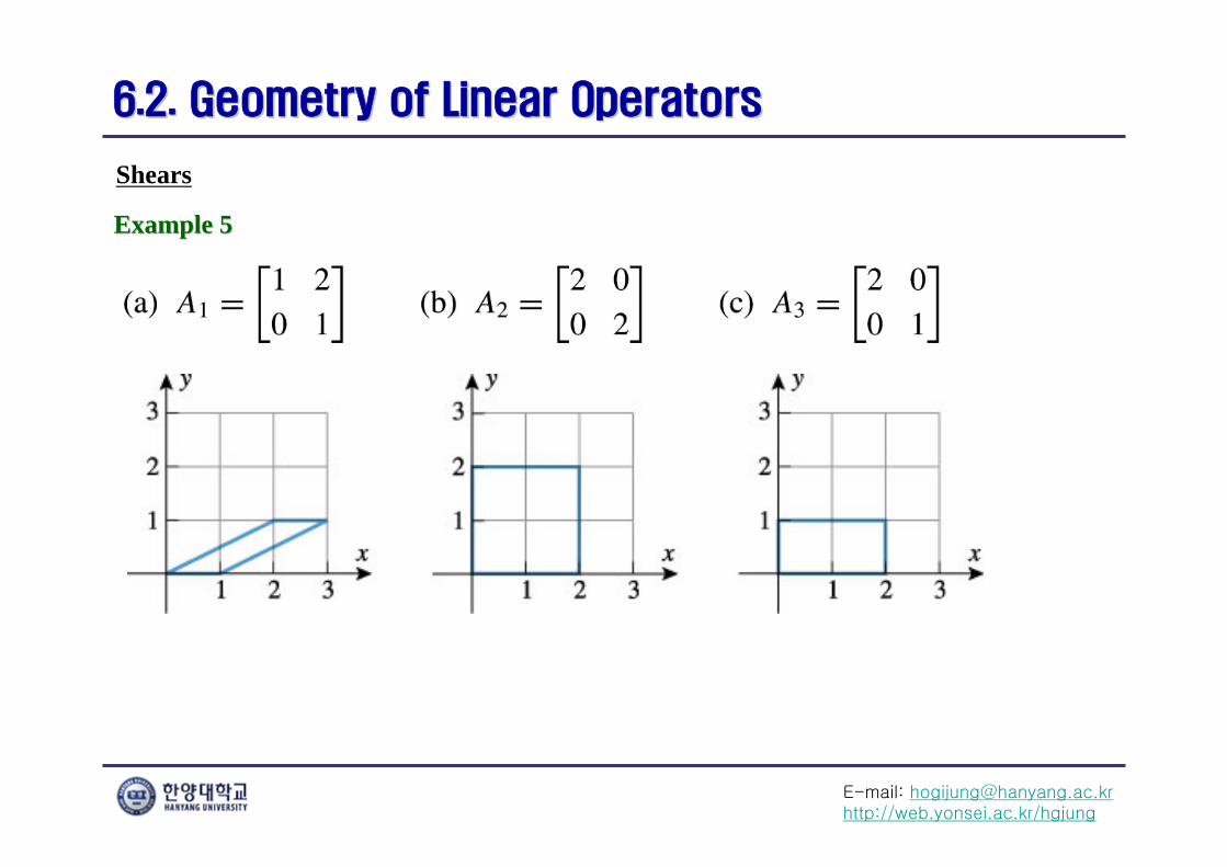
Shears
Example 5Example 5
E-mail: [email protected]://web.yonsei.ac.kr/hgjung
6.2. Geometry of Linear Operators6.2. Geometry of Linear Operators
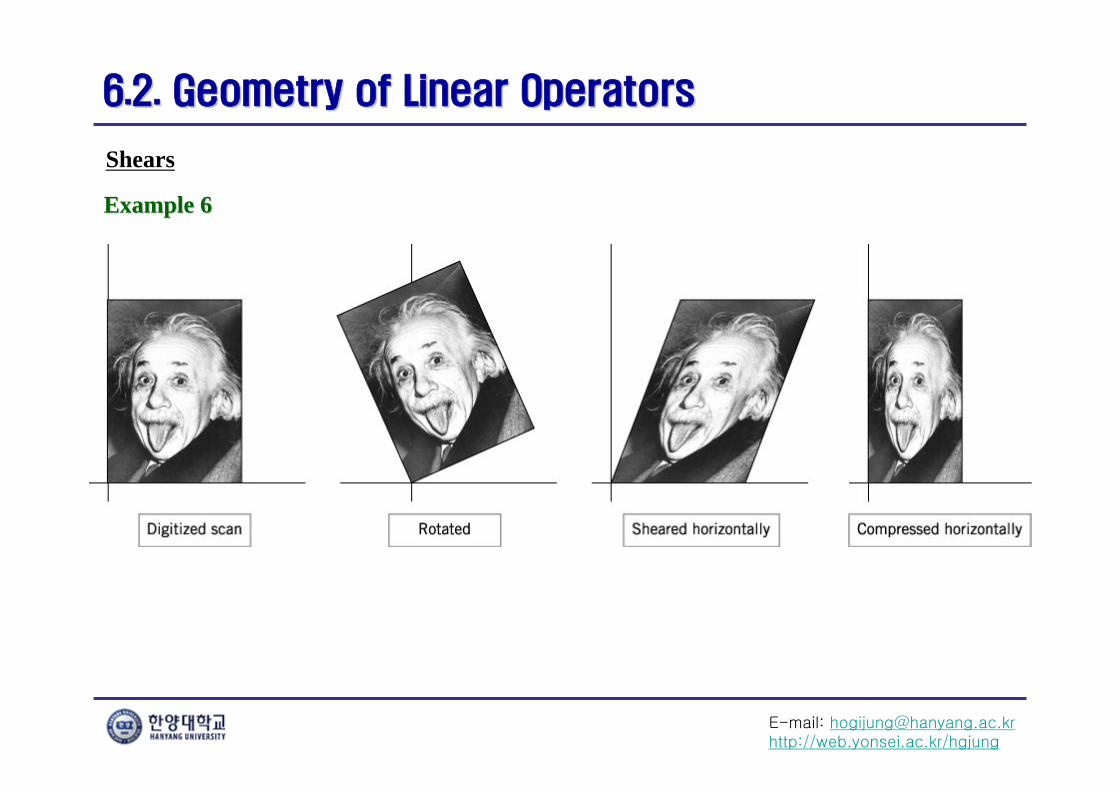
Shears
Example 6Example 6
E-mail: [email protected]://web.yonsei.ac.kr/hgjung
6.2. Geometry of Linear Operators6.2. Geometry of Linear Operators
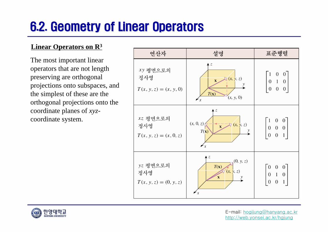
Linear Operators on R3
The most important linear operators that are not length preserving are orthogonal projections onto subspaces, and the simplest of these are the orthogonal projections onto the coordinate planes of xyz-coordinate system.
E-mail: [email protected]://web.yonsei.ac.kr/hgjung
6.2. Geometry of Linear Operators6.2. Geometry of Linear Operators
Linear Operators on R3
All 3×3 orthogonal matrices correspond to linear operators on R3 of the following types:
Type 1: Rotations about lines through the origin
Type 2: Reflections about planes through the origin
Type 3: A rotation about a line through the origin followed by a reflection about the plane through the origin that is perpendicular to the line
If A is a 3×3 orthogonal matrix, then A represents a rotations (i.e., is of type 1) if det(A)=1 and represents a type 2 or type 3 operator if det(A)=-1.
Accordingly, we will frequently refer to 2×2 or 3×3 orthogonal matrices with determinant 1 as rotation matrices.
E-mail: [email protected]://web.yonsei.ac.kr/hgjung
6.2. Geometry of Linear Operators6.2. Geometry of Linear Operators
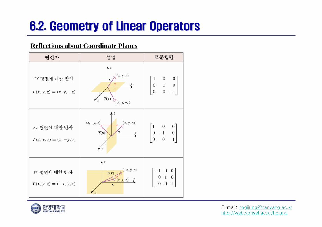
Reflections about Coordinate Planes
E-mail: [email protected]://web.yonsei.ac.kr/hgjung
6.2. Geometry of Linear Operators6.2. Geometry of Linear Operators
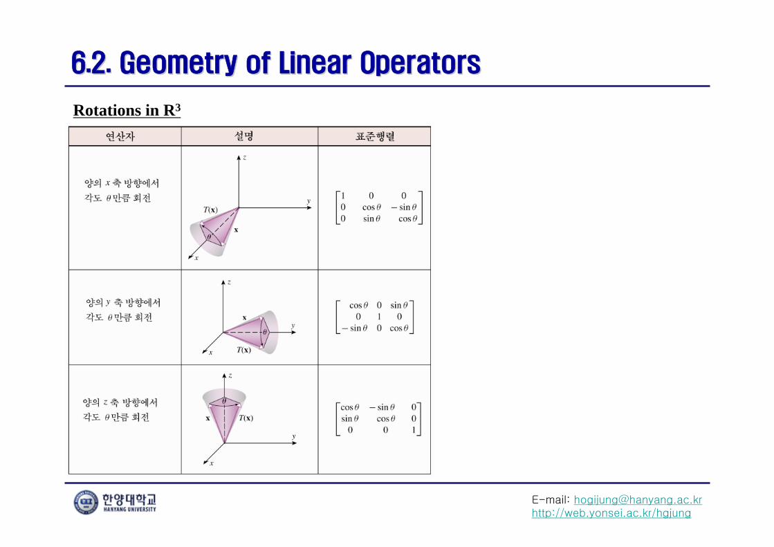
Rotations in R3
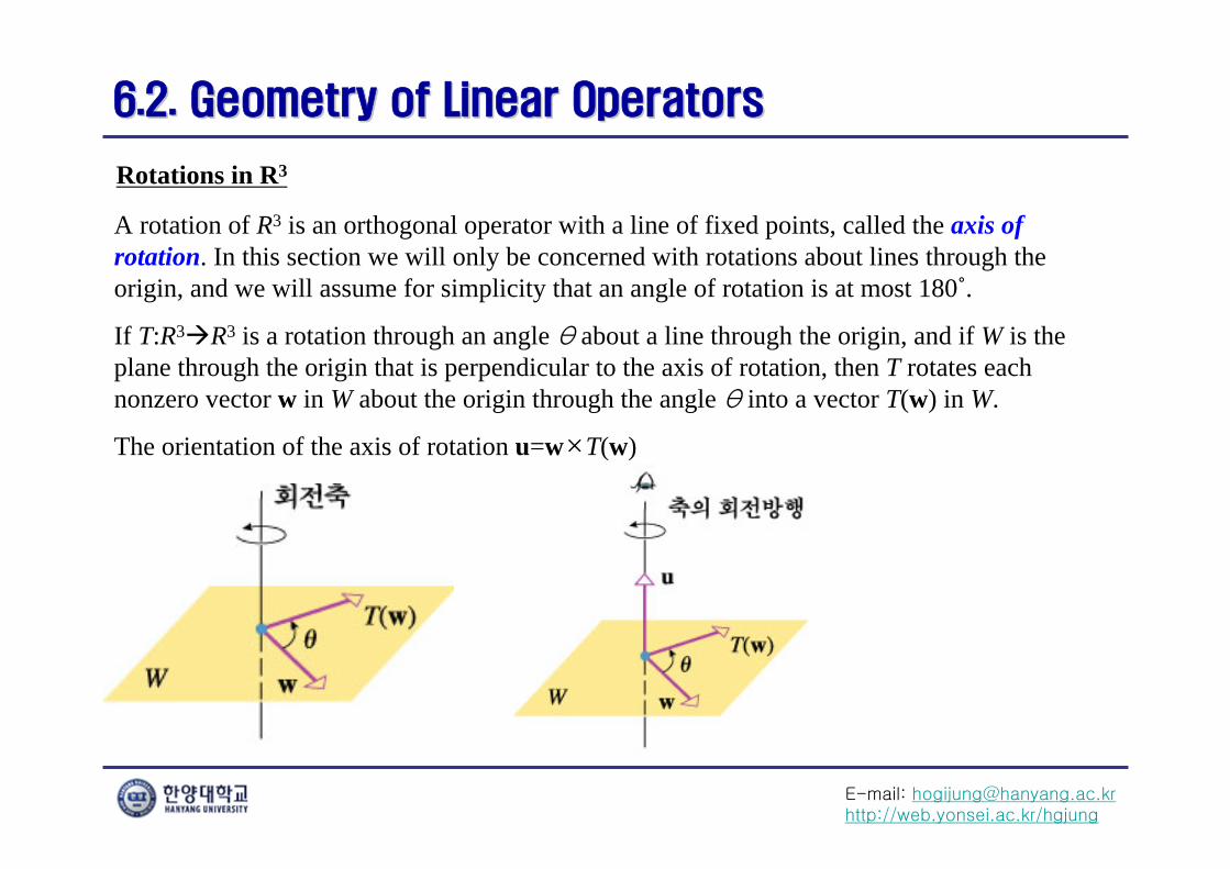
A rotation of R3 is an orthogonal operator with a line of fixed points, called the axis of rotation. In this section we will only be concerned with rotations about lines through the origin, and we will assume for simplicity that an angle of rotation is at most 180˚.
If T:R3R3 is a rotation through an angle θ about a line through the origin, and if W is the plane through the origin that is perpendicular to the axis of rotation, then T rotates each nonzero vector w in W about the origin through the angle θ into a vector T(w) in W.
The orientation of the axis of rotation u=w×T(w)
E-mail: [email protected]://web.yonsei.ac.kr/hgjung
6.2. Geometry of Linear Operators6.2. Geometry of Linear Operators
Rotations in R3
E-mail: [email protected]://web.yonsei.ac.kr/hgjung
6.2. Geometry of Linear Operators6.2. Geometry of Linear Operators
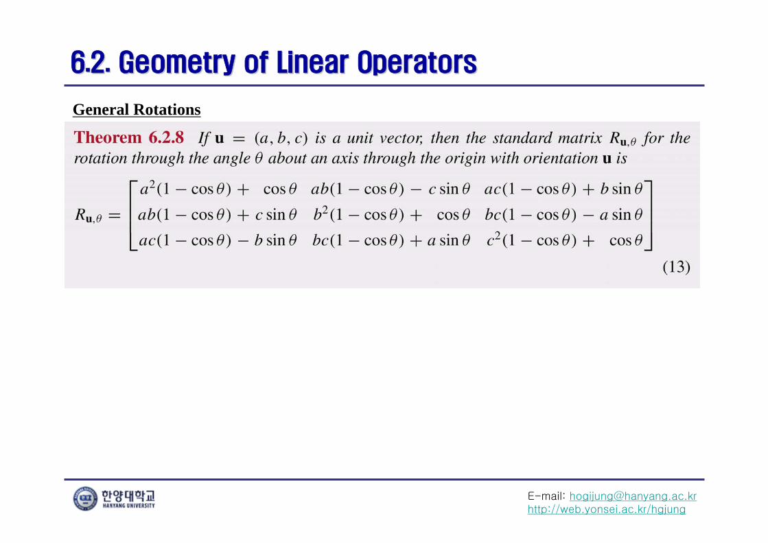
General Rotations
E-mail: [email protected]://web.yonsei.ac.kr/hgjung
6.2. Geometry of Linear Operators6.2. Geometry of Linear Operators
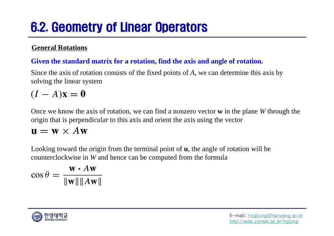
General Rotations
Given the standard matrix for a rotation, find the axis and angle of rotation.Since the axis of rotation consists of the fixed points of A, we can determine this axis by solving the linear system
Once we know the axis of rotation, we can find a nonzero vector w in the plane W through the origin that is perpendicular to this axis and orient the axis using the vector
Looking toward the origin from the terminal point of u, the angle of rotation will be counterclockwise in W and hence can be computed from the formula
E-mail: [email protected]://web.yonsei.ac.kr/hgjung
6.2. Geometry of Linear Operators6.2. Geometry of Linear Operators
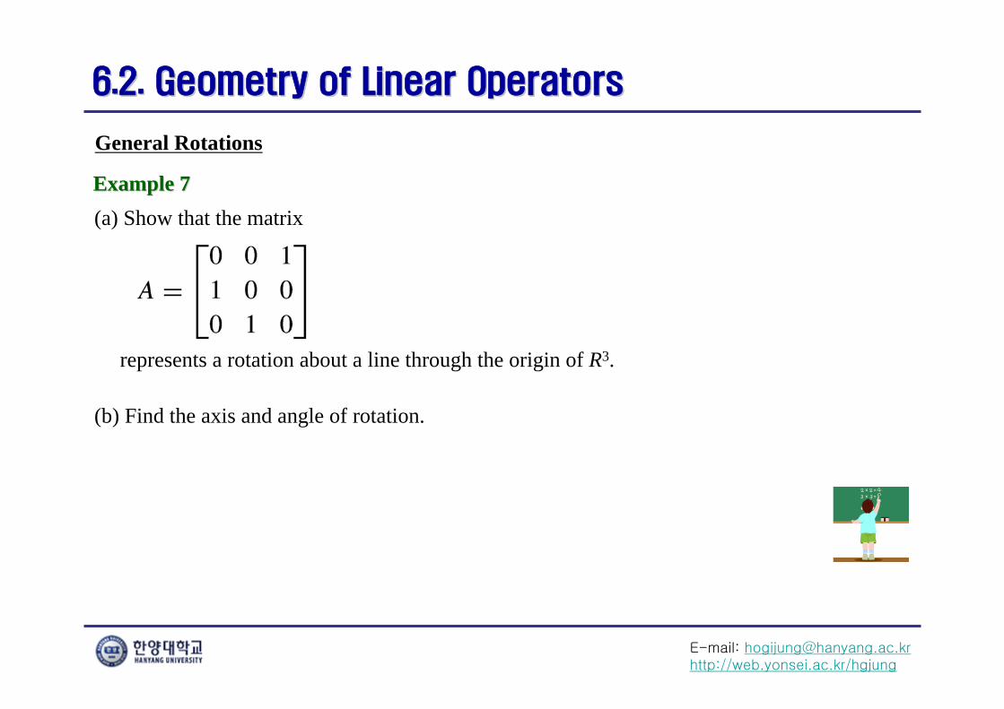
General Rotations
(a) Show that the matrixExample 7Example 7
represents a rotation about a line through the origin of R3.
(b) Find the axis and angle of rotation.
E-mail: [email protected]://web.yonsei.ac.kr/hgjung
6.2. Geometry of Linear Operators6.2. Geometry of Linear Operators
General Rotations
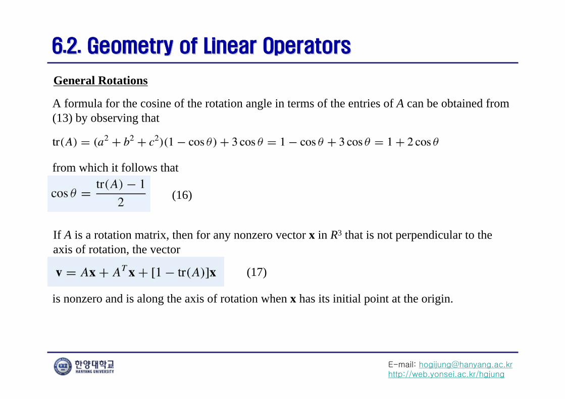
A formula for the cosine of the rotation angle in terms of the entries of A can be obtained from (13) by observing that
from which it follows that
If A is a rotation matrix, then for any nonzero vector x in R3 that is not perpendicular to the axis of rotation, the vector
is nonzero and is along the axis of rotation when x has its initial point at the origin.
(16)
(17)
E-mail: [email protected]://web.yonsei.ac.kr/hgjung
6.2. Geometry of Linear Operators6.2. Geometry of Linear Operators
General Rotations
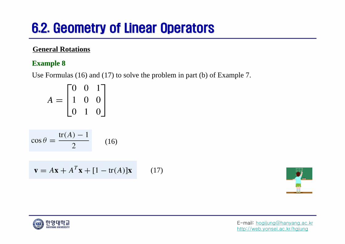
Use Formulas (16) and (17) to solve the problem in part (b) of Example 7.Example 8Example 8
(16)
(17)
E-mail: [email protected]://web.yonsei.ac.kr/hgjung
6.3. Kernel and Range6.3. Kernel and Range
Kernel of A Linear Transformation
In each part, find the kernel of the stated linear operator on R3.
(a) The zero operator T0(x)=0x=0: kel(T0)=R3
(b) The identity operator TI(x)=Ix=x: ker(TI)={0}
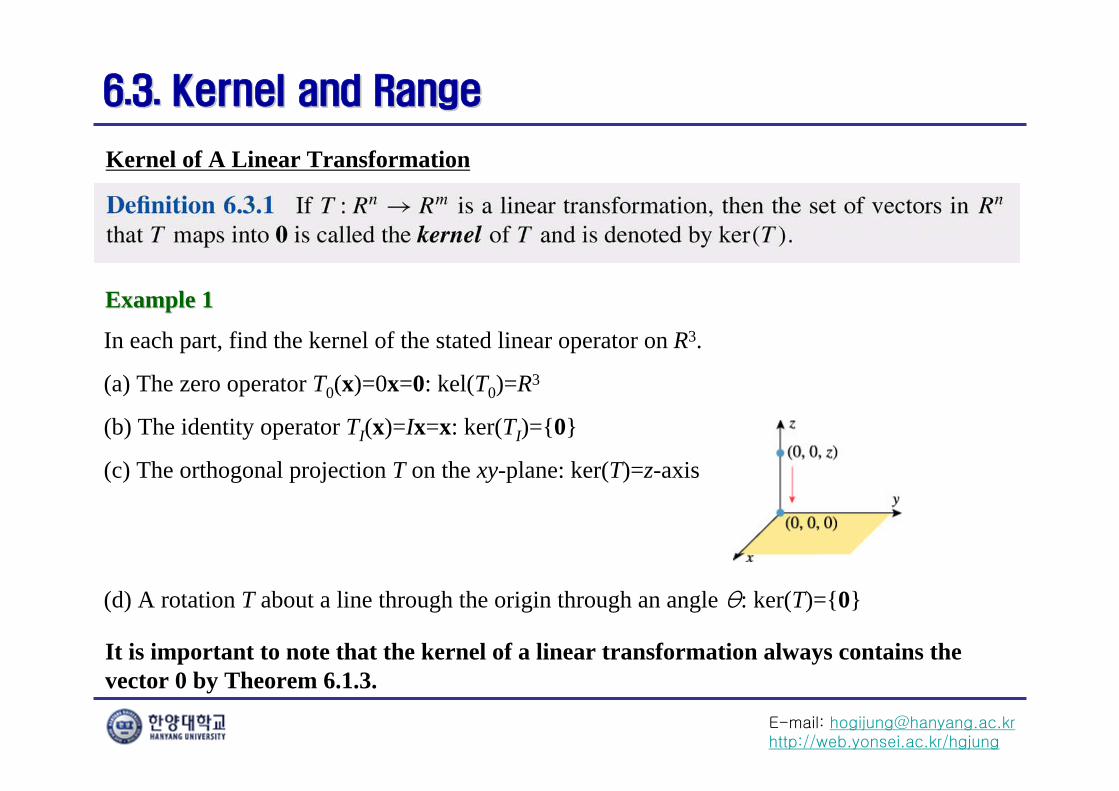
(c) The orthogonal projection T on the xy-plane: ker(T)=z-axis
(d) A rotation T about a line through the origin through an angle θ: ker(T)={0}
Example 1Example 1
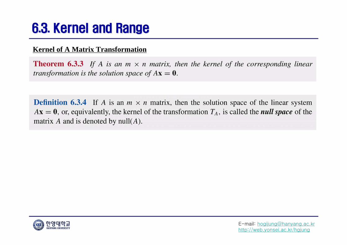
It is important to note that the kernel of a linear transformation always contains the vector 0 by Theorem 6.1.3.
E-mail: [email protected]://web.yonsei.ac.kr/hgjung
6.3. Kernel and Range6.3. Kernel and Range
Kernel of A Linear Transformation
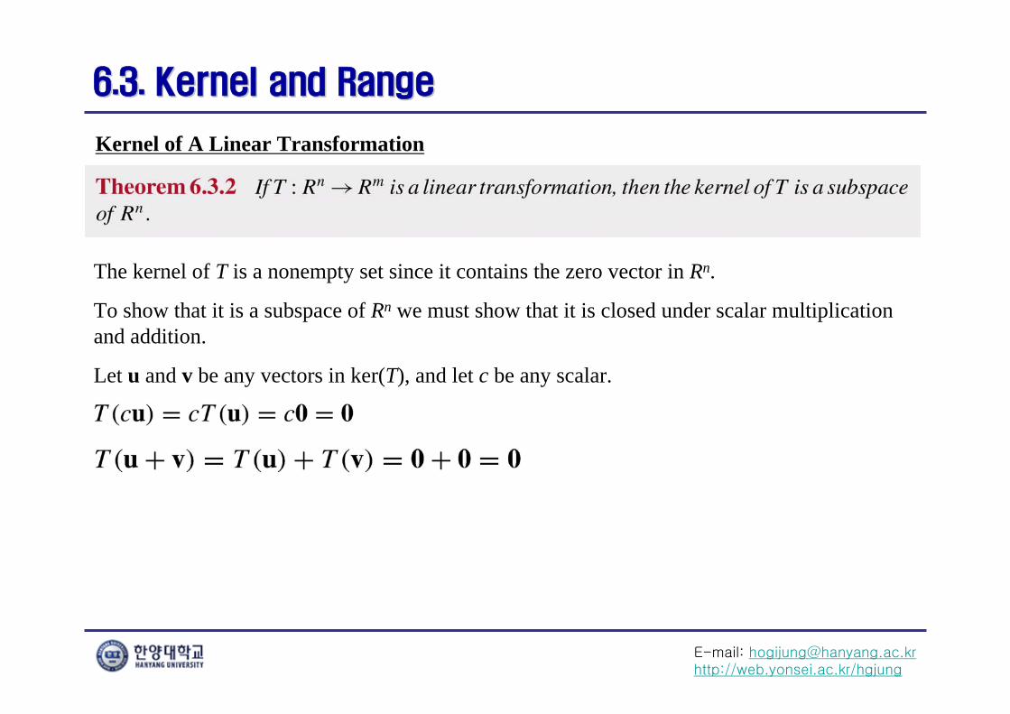
The kernel of T is a nonempty set since it contains the zero vector in Rn.
To show that it is a subspace of Rn we must show that it is closed under scalar multiplication and addition.
Let u and v be any vectors in ker(T), and let c be any scalar.
E-mail: [email protected]://web.yonsei.ac.kr/hgjung
6.3. Kernel and Range6.3. Kernel and Range
Kernel of A Matrix Transformation
E-mail: [email protected]://web.yonsei.ac.kr/hgjung
6.3. Kernel and Range6.3. Kernel and Range
Kernel of A Matrix Transformation
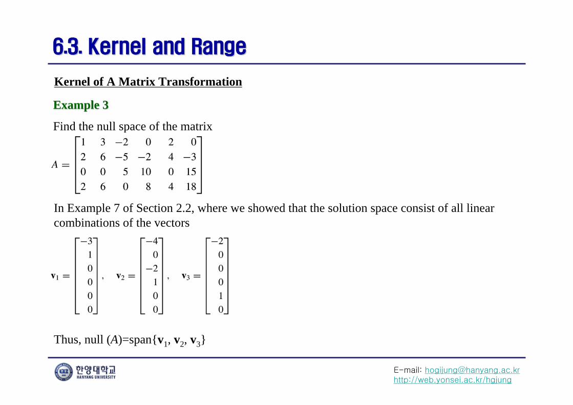
Find the null space of the matrix
Example 3Example 3
In Example 7 of Section 2.2, where we showed that the solution space consist of all linear combinations of the vectors
Thus, null (A)=span{v1, v2, v3}
E-mail: [email protected]://web.yonsei.ac.kr/hgjung
6.3. Kernel and Range6.3. Kernel and Range
Kernel of A Matrix Transformation
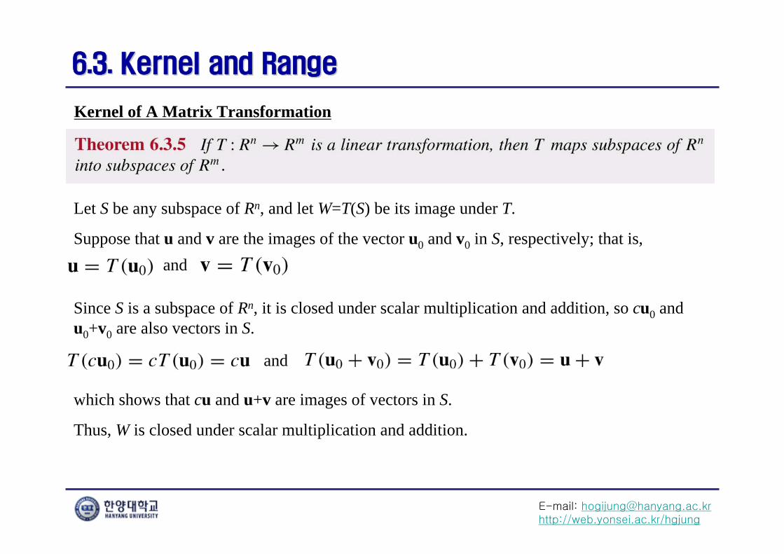
Let S be any subspace of Rn, and let W=T(S) be its image under T.
Suppose that u and v are the images of the vector u0 and v0 in S, respectively; that is,
Since S is a subspace of Rn, it is closed under scalar multiplication and addition, so cu0 and u0+v0 are also vectors in S.
and
and
which shows that cu and u+v are images of vectors in S.
Thus, W is closed under scalar multiplication and addition.
E-mail: [email protected]://web.yonsei.ac.kr/hgjung
6.3. Kernel and Range6.3. Kernel and Range
Range of A Linear Transformation
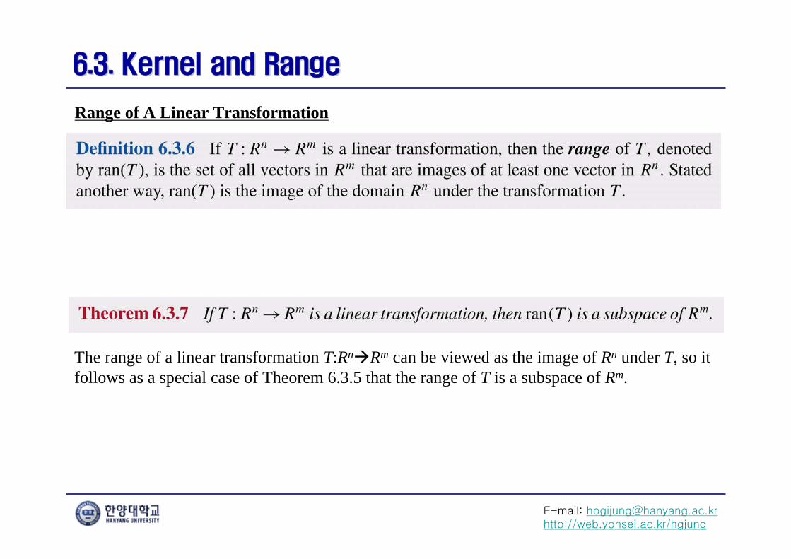
The range of a linear transformation T:RnRm can be viewed as the image of Rn under T, so it follows as a special case of Theorem 6.3.5 that the range of T is a subspace of Rm.
E-mail: [email protected]://web.yonsei.ac.kr/hgjung
6.3. Kernel and Range6.3. Kernel and Range
Range of A Matrix Transformation
If TA:RnRm is the linear transformation corresponding to the matrix A, then the range of TAand the column space of A are the same object from different points of view – the first emphasizes the transformation and the second the matrix.
E-mail: [email protected]://web.yonsei.ac.kr/hgjung
6.3. Kernel and Range6.3. Kernel and Range
Range of A Matrix Transformation
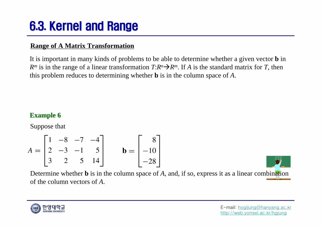
It is important in many kinds of problems to be able to determine whether a given vector b in Rm is in the range of a linear transformation T:RnRm. If A is the standard matrix for T, then this problem reduces to determining whether b is in the column space of A.
Example 6Example 6Suppose that
Determine whether b is in the column space of A, and, if so, express it as a linear combination of the column vectors of A.
E-mail: [email protected]://web.yonsei.ac.kr/hgjung
6.3. Kernel and Range6.3. Kernel and Range
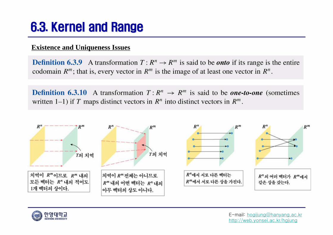
Existence and Uniqueness Issues
E-mail: [email protected]://web.yonsei.ac.kr/hgjung
6.3. Kernel and Range6.3. Kernel and Range
Existence and Uniqueness Issues
The rotation is onto and one-to-one.Example 7Example 7
Example 8Example 8
The orthogonal projection is neither onto nor one-to-one.
Example 9Example 9
T(x,y)=(x,y,0) is one-to-one, but is not onto.
Example 10Example 10
T(x,y,z)=(x,y) is onto, but is not one-to-one.
E-mail: [email protected]://web.yonsei.ac.kr/hgjung
6.3. Kernel and Range6.3. Kernel and Range
Existence and Uniqueness Issues
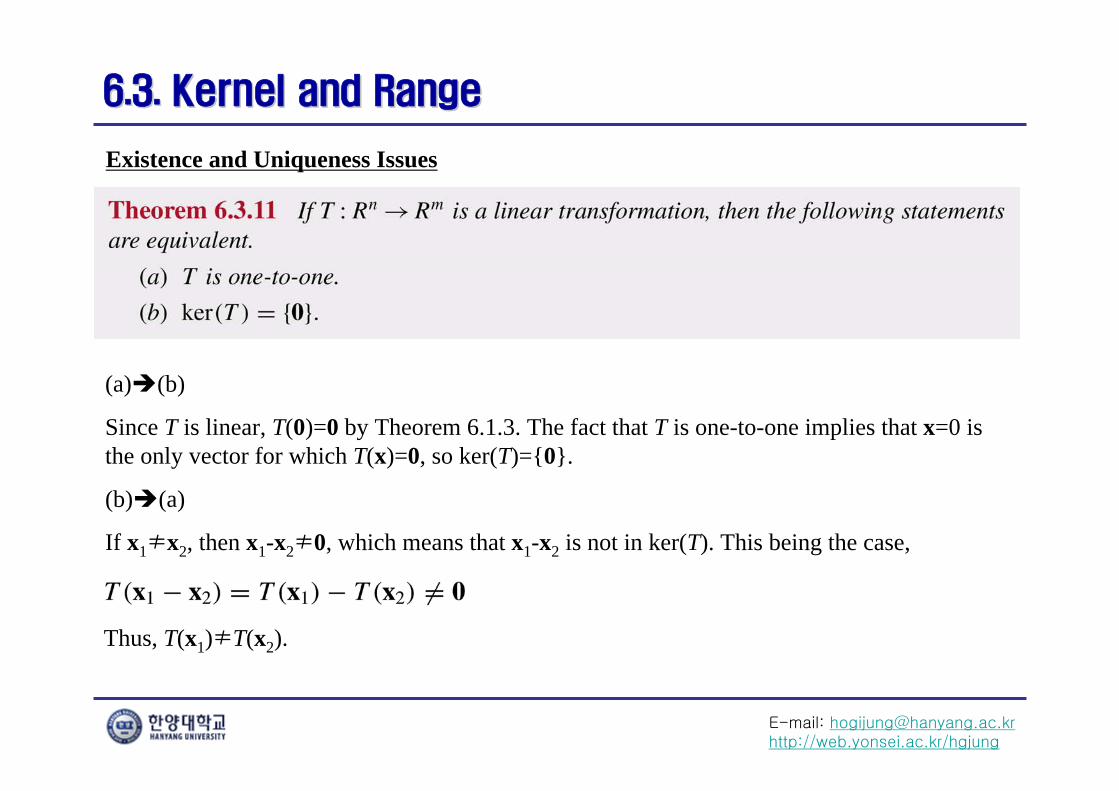
(a)(b)
Since T is linear, T(0)=0 by Theorem 6.1.3. The fact that T is one-to-one implies that x=0 is the only vector for which T(x)=0, so ker(T)={0}.
(b)(a)
If x1≠x2, then x1-x2≠0, which means that x1-x2 is not in ker(T). This being the case,
Thus, T(x1)≠T(x2).
E-mail: [email protected]://web.yonsei.ac.kr/hgjung
6.3. Kernel and Range6.3. Kernel and Range
Existence and Uniqueness Issues
E-mail: [email protected]://web.yonsei.ac.kr/hgjung
6.3. Kernel and Range6.3. Kernel and Range
Existence and Uniqueness Issues
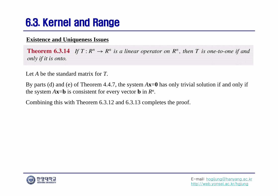
Let A be the standard matrix for T.
By parts (d) and (e) of Theorem 4.4.7, the system Ax=0 has only trivial solution if and only if the system Ax=b is consistent for every vector b in Rn.
Combining this with Theorem 6.3.12 and 6.3.13 completes the proof.
E-mail: [email protected]://web.yonsei.ac.kr/hgjung
6.3. Kernel and Range6.3. Kernel and Range
A Unifying Theorem
E-mail: [email protected]://web.yonsei.ac.kr/hgjung
6.3. Kernel and Range6.3. Kernel and Range
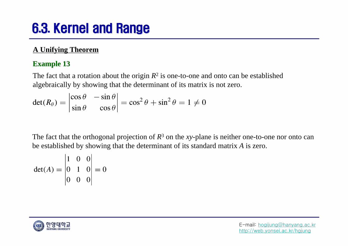
The fact that a rotation about the origin R2 is one-to-one and onto can be established algebraically by showing that the determinant of its matrix is not zero.
A Unifying Theorem
Example 13Example 13
The fact that the orthogonal projection of R3 on the xy-plane is neither one-to-one nor onto can be established by showing that the determinant of its standard matrix A is zero.
E-mail: [email protected]://web.yonsei.ac.kr/hgjung
6.4. Composition and Invertibility6.4. Composition and Invertibility
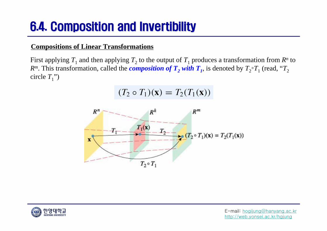
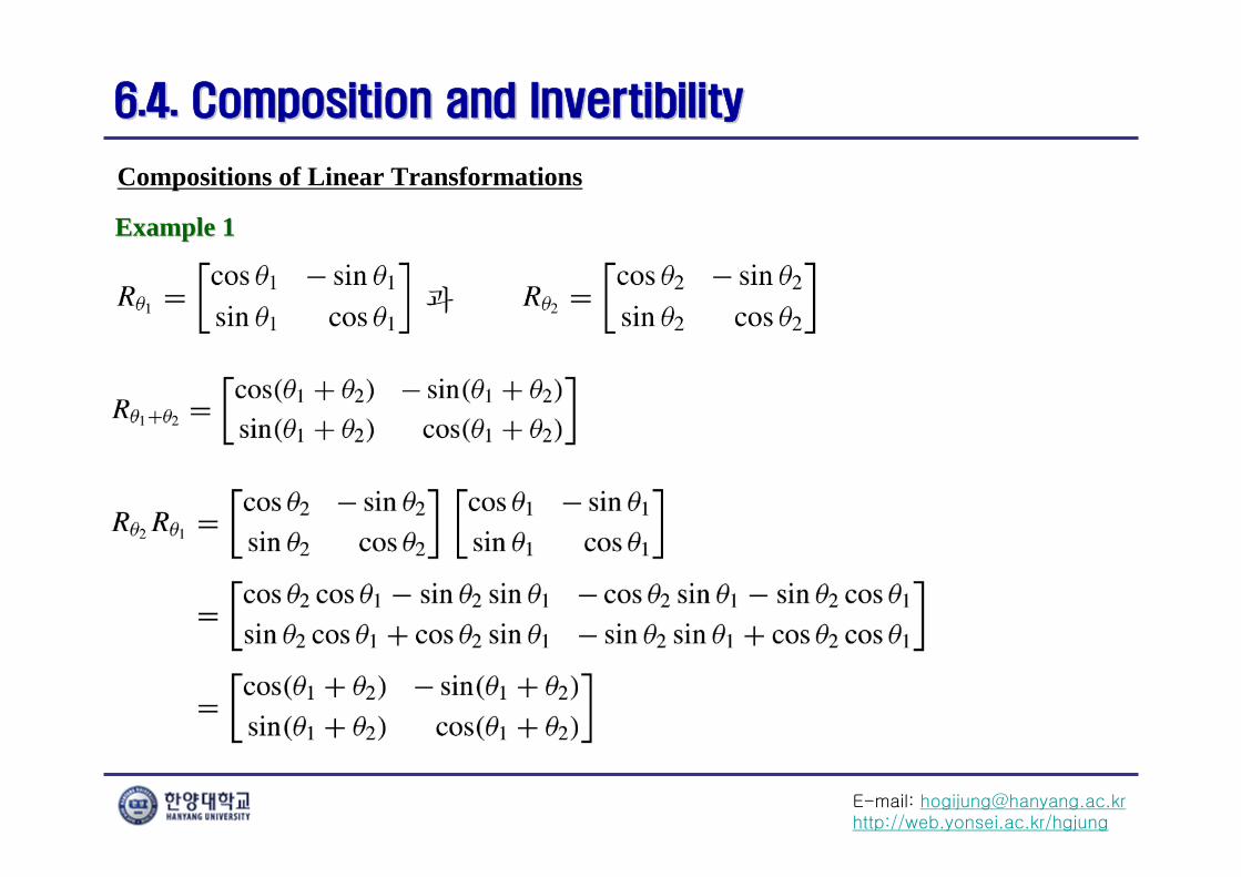
Compositions of Linear Transformations
First applying T1 and then applying T2 to the output of T1 produces a transformation from Rn to Rm. This transformation, called the composition of T2 with T1, is denoted by T2◦T1 (read, “T2circle T1”)
E-mail: [email protected]://web.yonsei.ac.kr/hgjung
6.4. Composition and Invertibility6.4. Composition and Invertibility
Compositions of Linear Transformations
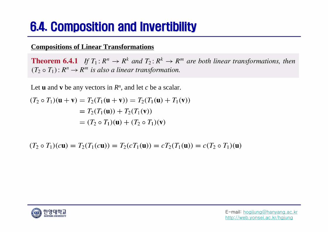
Let u and v be any vectors in Rn, and let c be a scalar.
E-mail: [email protected]://web.yonsei.ac.kr/hgjung
6.4. Composition and Invertibility6.4. Composition and Invertibility
Compositions of Linear Transformations
E-mail: [email protected]://web.yonsei.ac.kr/hgjung
6.4. Composition and Invertibility6.4. Composition and Invertibility
Compositions of Linear Transformations
Example 1Example 1
E-mail: [email protected]://web.yonsei.ac.kr/hgjung
6.4. Composition and Invertibility6.4. Composition and Invertibility
Compositions of Linear Transformations
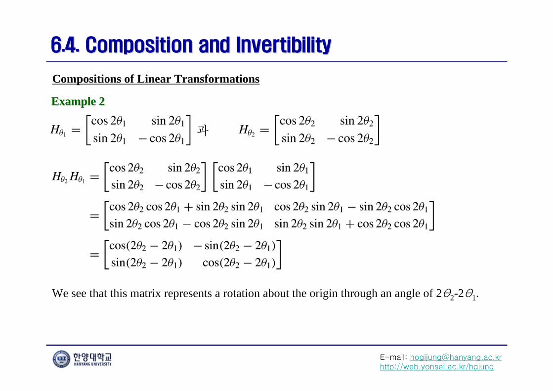
Example 2Example 2
We see that this matrix represents a rotation about the origin through an angle of 2θ2-2θ1.
E-mail: [email protected]://web.yonsei.ac.kr/hgjung
6.4. Composition and Invertibility6.4. Composition and Invertibility
Compositions of Linear Transformations
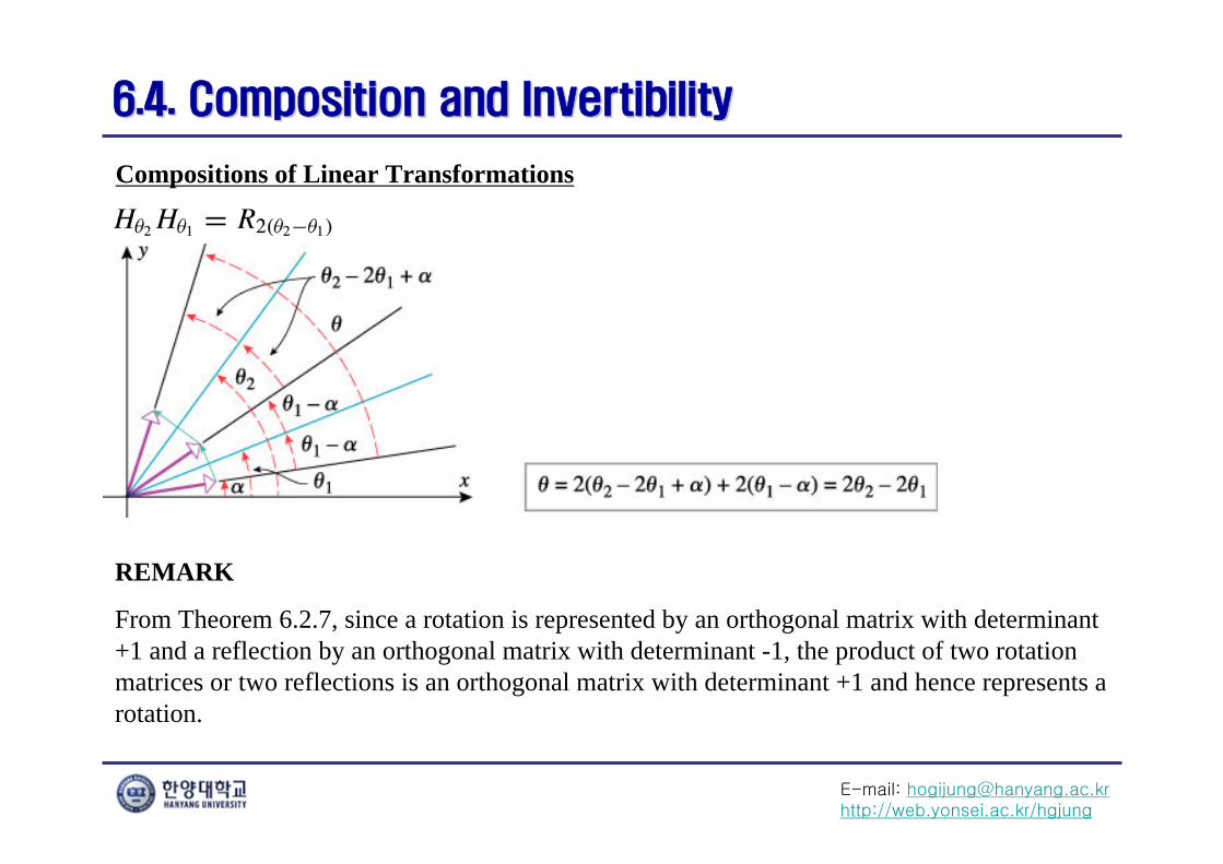
REMARK
From Theorem 6.2.7, since a rotation is represented by an orthogonal matrix with determinant +1 and a reflection by an orthogonal matrix with determinant -1, the product of two rotation matrices or two reflections is an orthogonal matrix with determinant +1 and hence represents a rotation.
E-mail: [email protected]://web.yonsei.ac.kr/hgjung
6.4. Composition and Invertibility6.4. Composition and Invertibility
Compositions of Linear Transformations
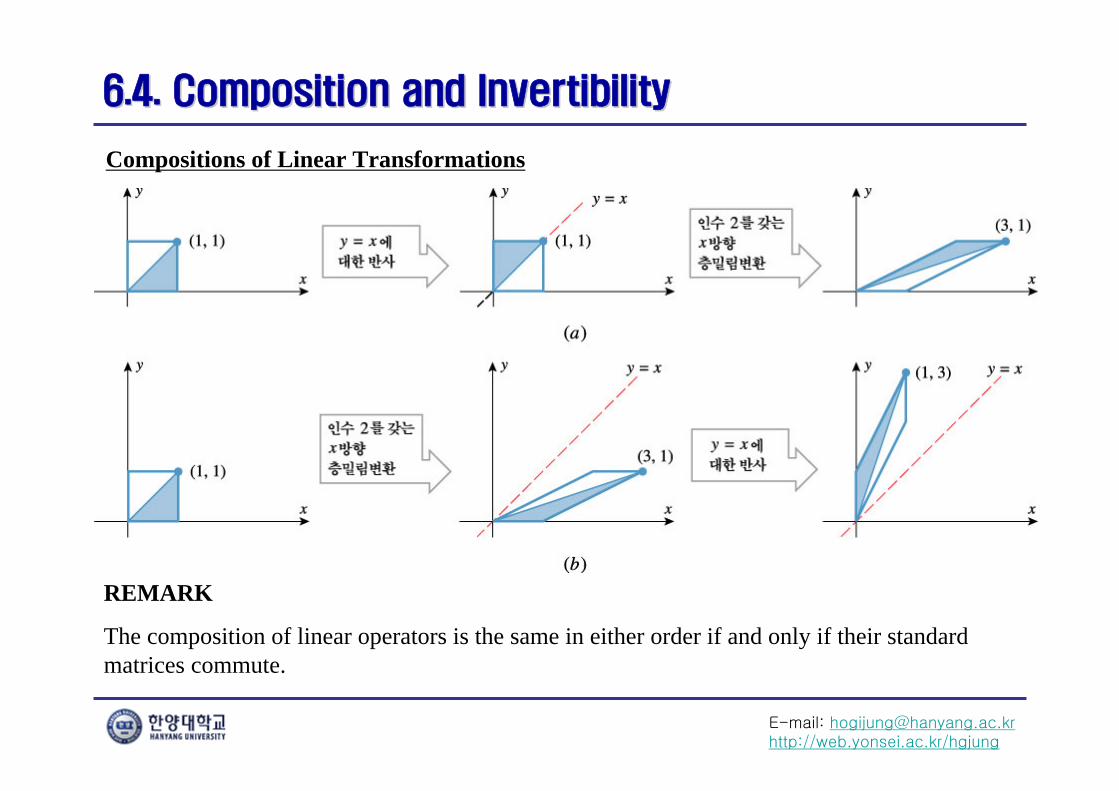
REMARK
The composition of linear operators is the same in either order if and only if their standard matrices commute.
E-mail: [email protected]://web.yonsei.ac.kr/hgjung
6.4. Composition and Invertibility6.4. Composition and Invertibility
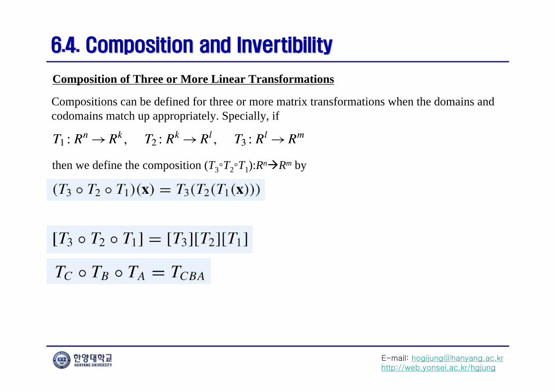
Composition of Three or More Linear Transformations
Compositions can be defined for three or more matrix transformations when the domains and codomains match up appropriately. Specially, if
then we define the composition (T3◦T2◦T1):RnRm by

E-mail: [email protected]://web.yonsei.ac.kr/hgjung
6.4. Composition and Invertibility6.4. Composition and Invertibility
Composition of Three or More Linear Transformations
Let A1, A2, …, Ak be the standard matrices for the rotations. Each matrix is orthogonal and has determinant 1, so the same is true for the product
Thus, A represents a rotation about some axis through the origin of R3. Since A is the standard matrix for the composition Tk◦T2◦T1, the result is proved.
E-mail: [email protected]://web.yonsei.ac.kr/hgjung
6.4. Composition and Invertibility6.4. Composition and Invertibility
Composition of Three or More Linear Transformations
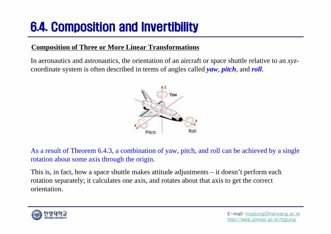
In aeronautics and astronautics, the orientation of an aircraft or space shuttle relative to an xyz-coordinate system is often described in terms of angles called yaw, pitch, and roll.
As a result of Theorem 6.4.3, a combination of yaw, pitch, and roll can be achieved by a single rotation about some axis through the origin.
This is, in fact, how a space shuttle makes attitude adjustments – it doesn’t perform each rotation separately; it calculates one axis, and rotates about that axis to get the correct orientation.
E-mail: [email protected]://web.yonsei.ac.kr/hgjung
6.4. Composition and Invertibility6.4. Composition and Invertibility
Composition of Three or More Linear Transformations
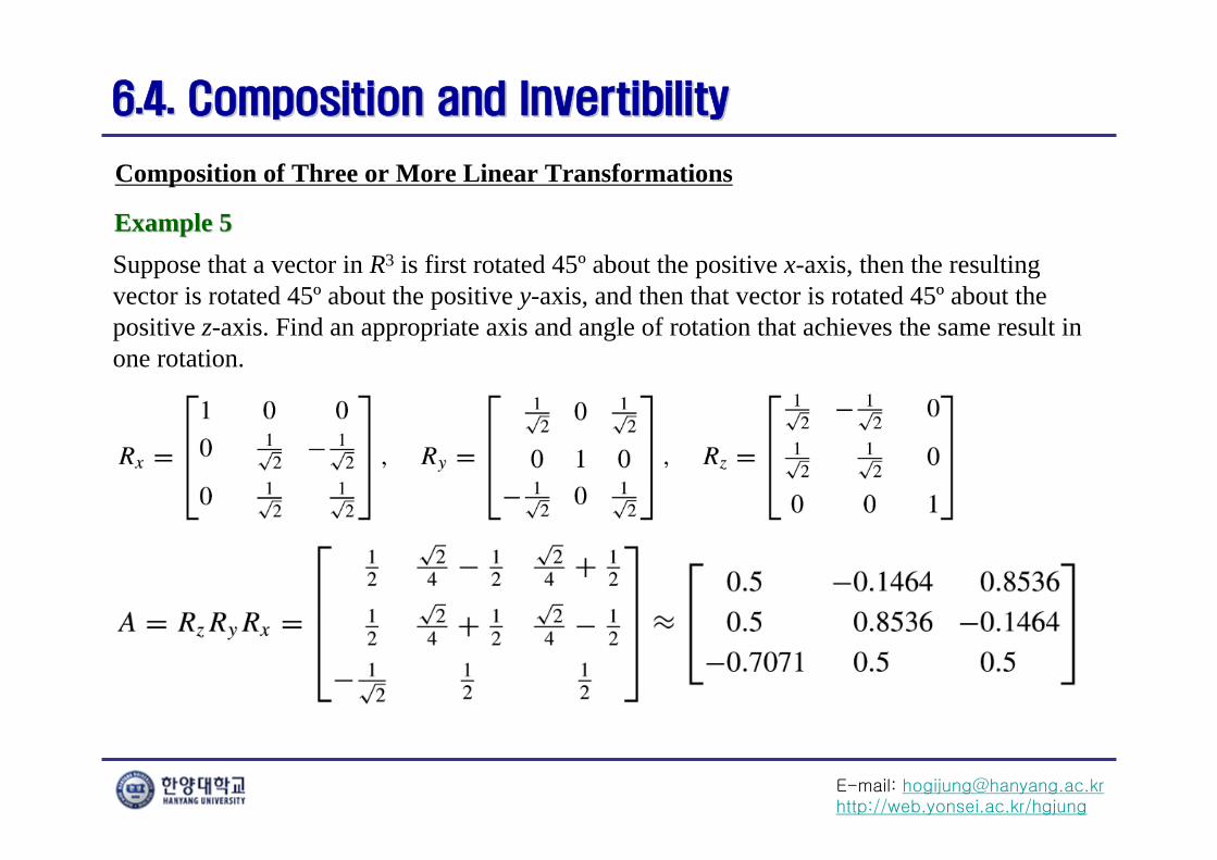
Suppose that a vector in R3 is first rotated 45º about the positive x-axis, then the resulting vector is rotated 45º about the positive y-axis, and then that vector is rotated 45º about the positive z-axis. Find an appropriate axis and angle of rotation that achieves the same result in one rotation.
Example 5Example 5

E-mail: [email protected]://web.yonsei.ac.kr/hgjung
6.4. Composition and Invertibility6.4. Composition and Invertibility
Composition of Three or More Linear Transformations
To find the axis of rotation v we will apply Formula (17) of Section 6.2, taking the arbitrary vector x to be e1.
Example 5Example 5
(16)
(17)
Also, it follows from Formula (16) of Section 6.2 that the angle of rotation satisfies
from which it follows that θ ≈ 64.74º
E-mail: [email protected]://web.yonsei.ac.kr/hgjung
6.4. Composition and Invertibility6.4. Composition and Invertibility
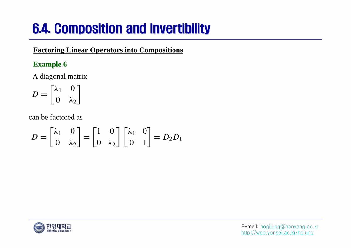
Factoring Linear Operators into Compositions
A diagonal matrixExample 6Example 6
can be factored as
E-mail: [email protected]://web.yonsei.ac.kr/hgjung
6.4. Composition and Invertibility6.4. Composition and Invertibility
Factoring Linear Operators into Compositions
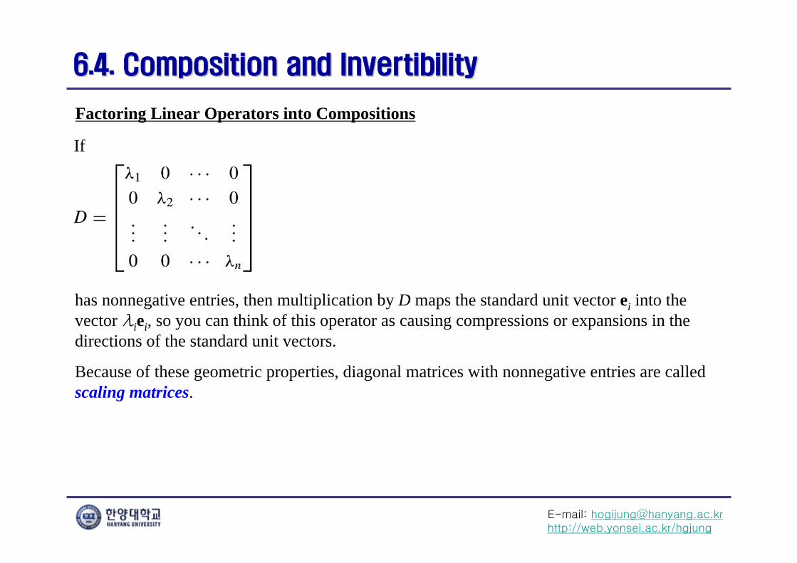
If
has nonnegative entries, then multiplication by D maps the standard unit vector ei into the vector λiei, so you can think of this operator as causing compressions or expansions in the directions of the standard unit vectors.
Because of these geometric properties, diagonal matrices with nonnegative entries are called scaling matrices.
E-mail: [email protected]://web.yonsei.ac.kr/hgjung
6.4. Composition and Invertibility6.4. Composition and Invertibility
Factoring Linear Operators into Compositions
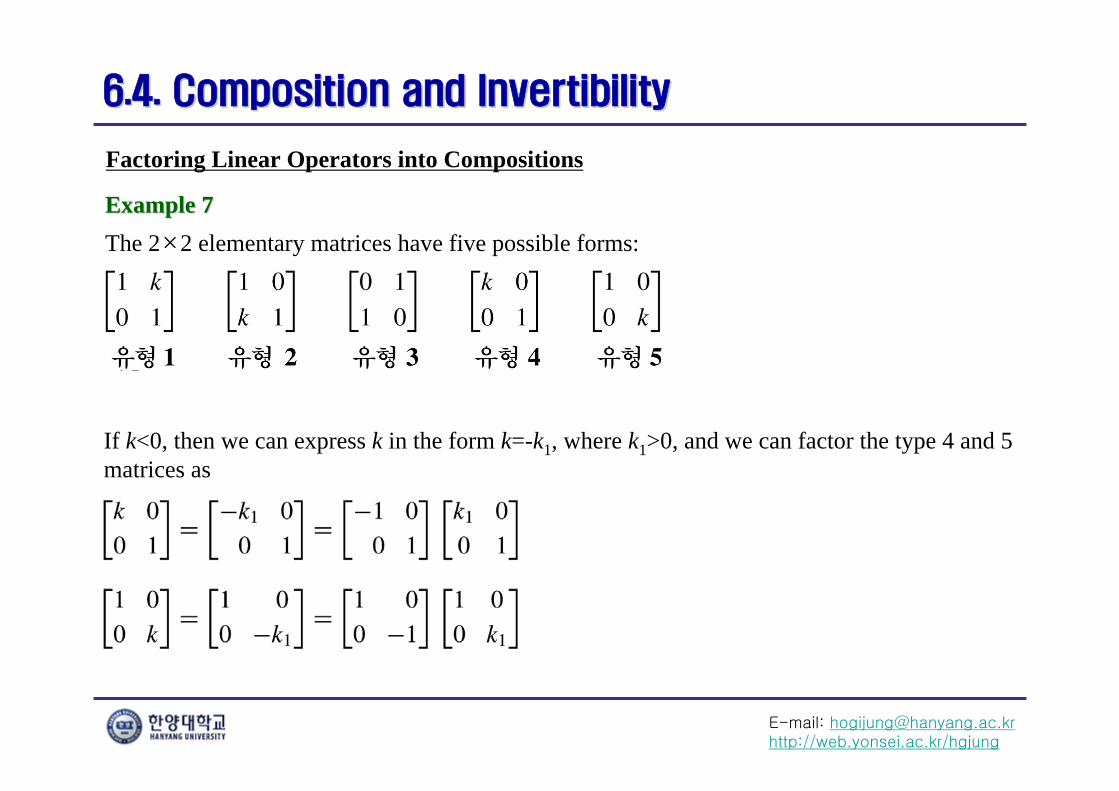
The 2×2 elementary matrices have five possible forms:Example 7Example 7
If k<0, then we can express k in the form k=-k1, where k1>0, and we can factor the type 4 and 5 matrices as
E-mail: [email protected]://web.yonsei.ac.kr/hgjung
6.4. Composition and Invertibility6.4. Composition and Invertibility
Factoring Linear Operators into Compositions
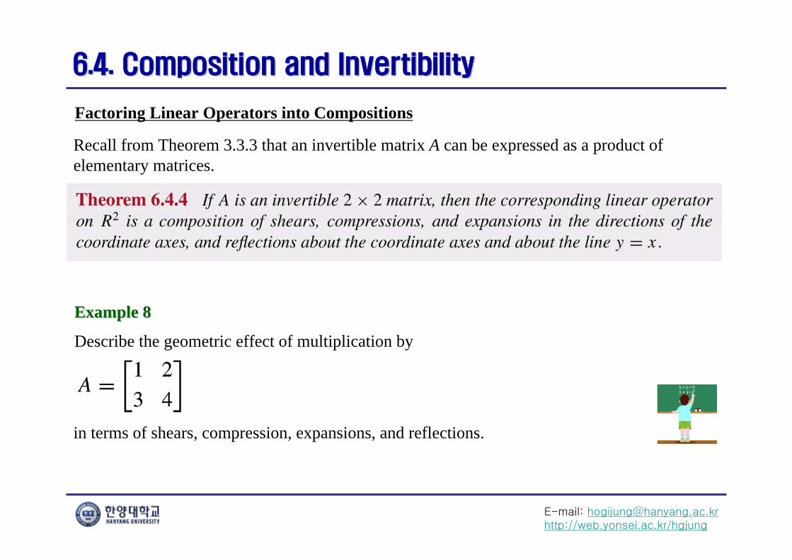
Recall from Theorem 3.3.3 that an invertible matrix A can be expressed as a product of elementary matrices.
Example 8Example 8
Describe the geometric effect of multiplication by
in terms of shears, compression, expansions, and reflections.
E-mail: [email protected]://web.yonsei.ac.kr/hgjung
6.4. Composition and Invertibility6.4. Composition and Invertibility
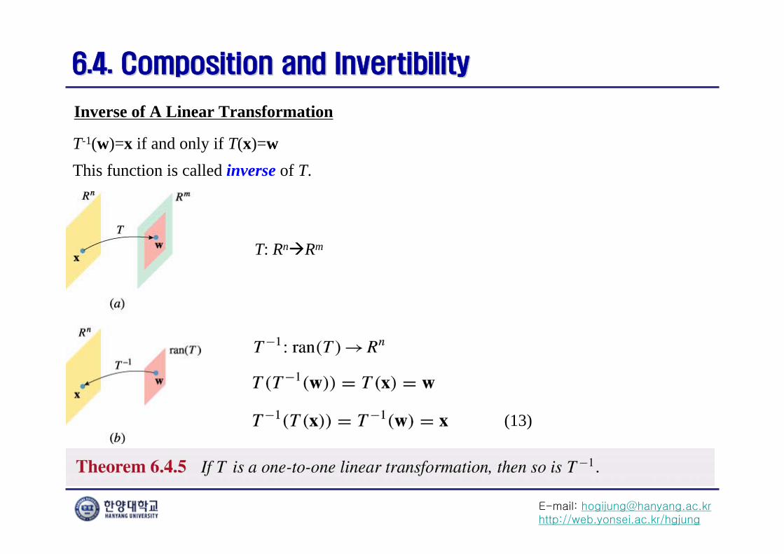
Inverse of A Linear Transformation
T-1(w)=x if and only if T(x)=wThis function is called inverse of T.
T: RnRm
(13)
E-mail: [email protected]://web.yonsei.ac.kr/hgjung
6.4. Composition and Invertibility6.4. Composition and Invertibility
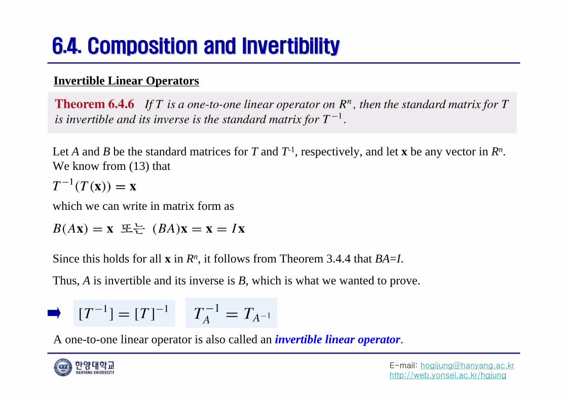
Invertible Linear Operators
Let A and B be the standard matrices for T and T-1, respectively, and let x be any vector in Rn. We know from (13) that
which we can write in matrix form as
Since this holds for all x in Rn, it follows from Theorem 3.4.4 that BA=I.
Thus, A is invertible and its inverse is B, which is what we wanted to prove.
A one-to-one linear operator is also called an invertible linear operator.
E-mail: [email protected]://web.yonsei.ac.kr/hgjung
6.4. Composition and Invertibility6.4. Composition and Invertibility
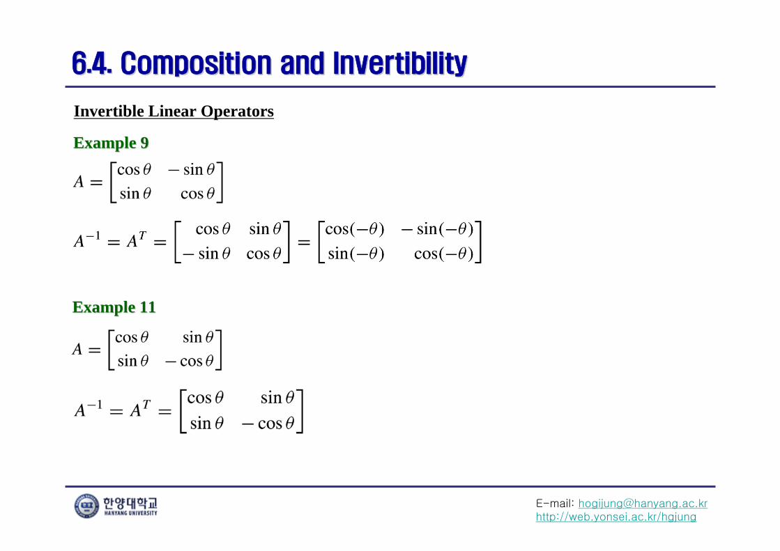
Invertible Linear Operators
Example 9Example 9
Example 11Example 11
E-mail: [email protected]://web.yonsei.ac.kr/hgjung
6.4. Composition and Invertibility6.4. Composition and Invertibility
Geometric Properties of Invertible Linear Operators on R2
E-mail: [email protected]://web.yonsei.ac.kr/hgjung
6.4. Composition and Invertibility6.4. Composition and Invertibility
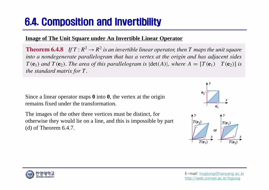
Image of The Unit Square under An Invertible Linear Operator
Since a linear operator maps 0 into 0, the vertex at the origin remains fixed under the transformation.
The images of the other three vertices must be distinct, for otherwise they would lie on a line, and this is impossible by part (d) of Theorem 6.4.7.
E-mail: [email protected]://web.yonsei.ac.kr/hgjung
6.5. Computer Graphics6.5. Computer Graphics
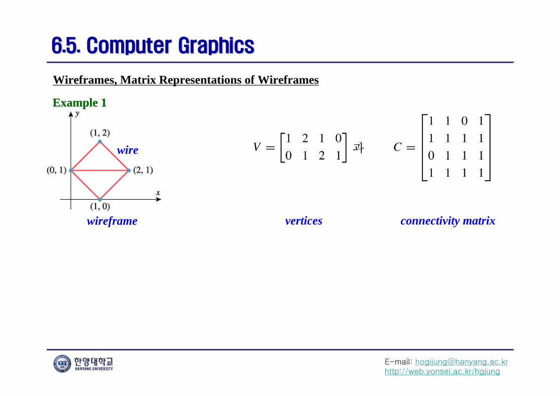
Wireframes, Matrix Representations of Wireframes
Example 1Example 1
vertices connectivity matrix
wire
wireframe
E-mail: [email protected]://web.yonsei.ac.kr/hgjung
6.5. Computer Graphics6.5. Computer Graphics
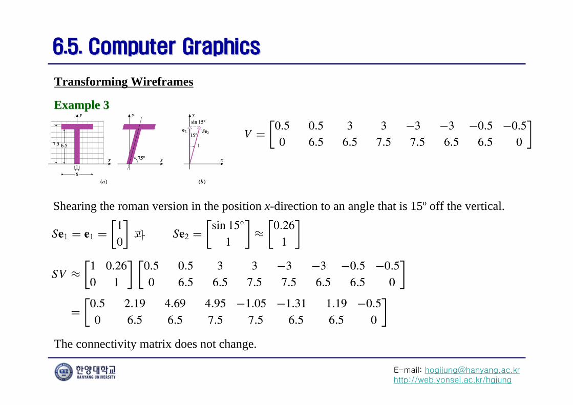
Transforming Wireframes
The connectivity matrix does not change.
Example 3Example 3
Shearing the roman version in the position x-direction to an angle that is 15º off the vertical.
E-mail: [email protected]://web.yonsei.ac.kr/hgjung
6.5. Computer Graphics6.5. Computer Graphics
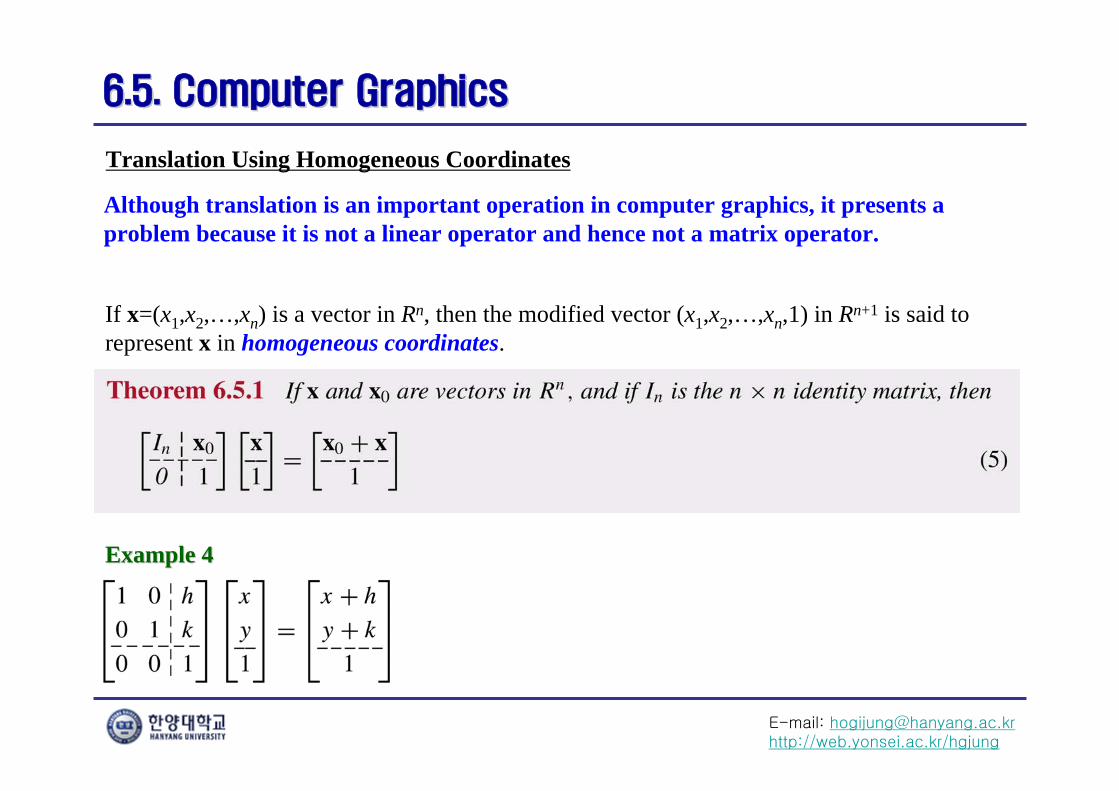
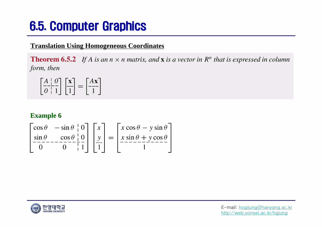
Translation Using Homogeneous Coordinates
If x=(x1,x2,…,xn) is a vector in Rn, then the modified vector (x1,x2,…,xn,1) in Rn+1 is said to represent x in homogeneous coordinates.
Although translation is an important operation in computer graphics, it presents a problem because it is not a linear operator and hence not a matrix operator.
Example 4Example 4
E-mail: [email protected]://web.yonsei.ac.kr/hgjung
6.5. Computer Graphics6.5. Computer Graphics
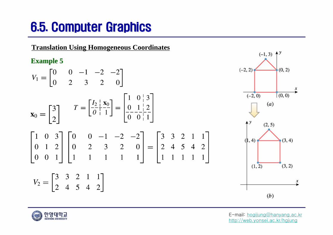
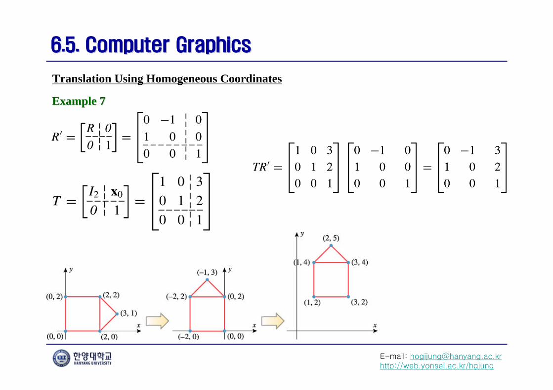
Translation Using Homogeneous Coordinates
Example 5Example 5
E-mail: [email protected]://web.yonsei.ac.kr/hgjung
6.5. Computer Graphics6.5. Computer Graphics
Translation Using Homogeneous Coordinates
Example 6Example 6
E-mail: [email protected]://web.yonsei.ac.kr/hgjung
6.5. Computer Graphics6.5. Computer Graphics
Translation Using Homogeneous Coordinates
Example 7Example 7
E-mail: [email protected]://web.yonsei.ac.kr/hgjung
6.5. Computer Graphics6.5. Computer Graphics
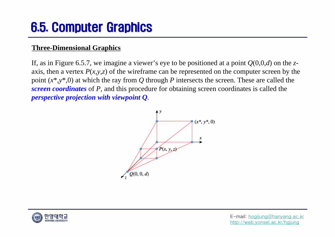
Three-Dimensional Graphics
If, as in Figure 6.5.7, we imagine a viewer’s eye to be positioned at a point Q(0,0,d) on the z-axis, then a vertex P(x,y,z) of the wireframe can be represented on the computer screen by the point (x*,y*,0) at which the ray from Q through P intersects the screen. These are called the screen coordinates of P, and this procedure for obtaining screen coordinates is called the perspective projection with viewpoint Q.
E-mail: [email protected]://web.yonsei.ac.kr/hgjung
6.5. Computer Graphics6.5. Computer Graphics
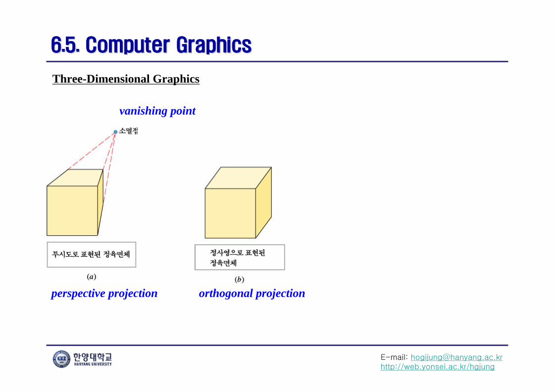
Three-Dimensional Graphics
orthogonal projectionperspective projection
vanishing point
E-mail: [email protected]://web.yonsei.ac.kr/hgjung
6.5. Computer Graphics6.5. Computer Graphics
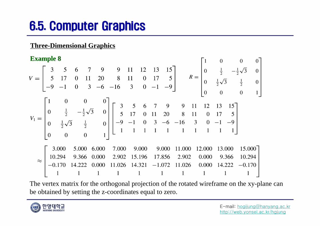
Three-Dimensional Graphics
The vertex matrix for the orthogonal projection of the rotated wireframe on the xy-plane can be obtained by setting the z-coordinates equal to zero.
Example 8Example 8
E-mail: [email protected]://web.yonsei.ac.kr/hgjung
6.5. Computer Graphics6.5. Computer Graphics
Three-Dimensional Graphics
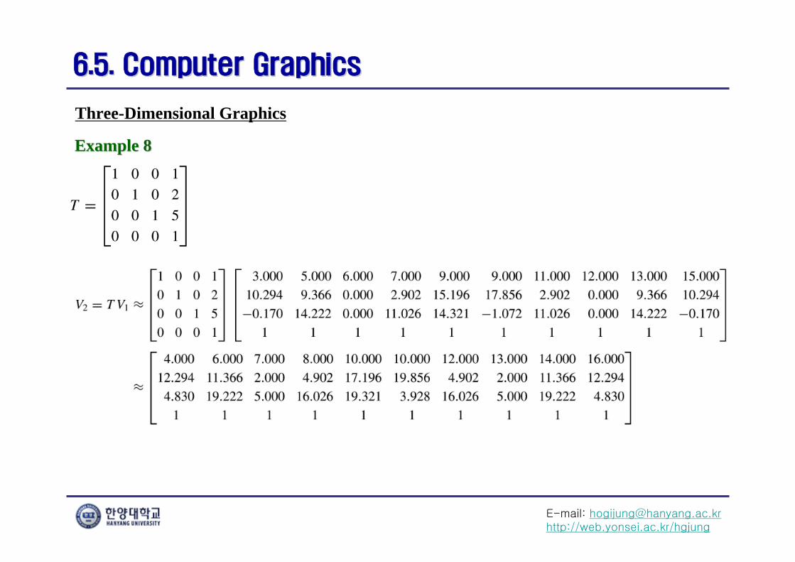
Example 8Example 8
E-mail: [email protected]://web.yonsei.ac.kr/hgjung
6.5. Computer Graphics6.5. Computer Graphics
Three-Dimensional Graphics
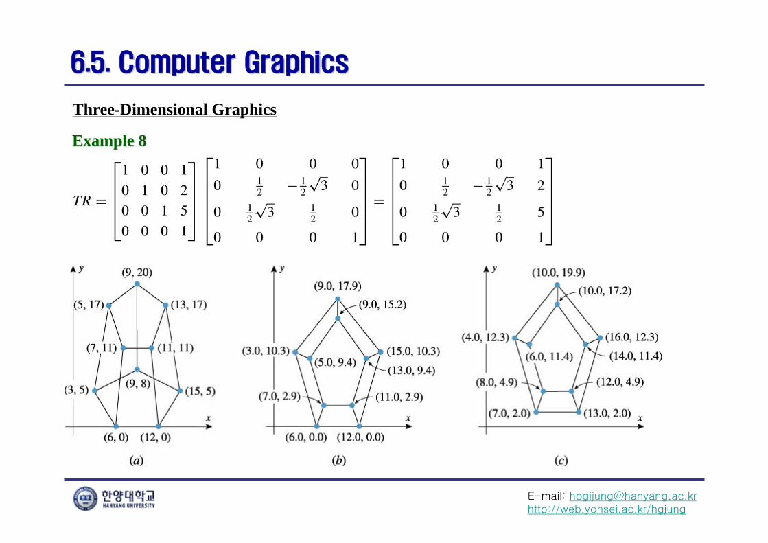
Example 8Example 8